Using Microsoft Excel3 Formatting

Using Microsoft Excel Formatting

Using Microsoft Excel
Formatting a Spreadsheet
Formatting a spreadsheet means changing the way it looks to make it
neater and more attractive. Formatting changes can include
modifying number styles, text size and colours. Many people format
their spreadsheet as they go but a lot of time and effort can be saved
by waiting until the sheet it relatively complete before worrying
about the formatting. This is because it is a lot easier to format a sheet once it already has a good
amount of content.
Formatting a spreadsheet can be done in a number of different ways:
• Using AutoFormat
• Using toolbar icons and shortcuts
• Using the format cells dialog box

That later methods take more time and effort but allow for far greater control over the end result.

© Stephen O’Neil 2005 Page 1 Of 12 www.oneil.com.au/pc


Using AutoFormat
Excel’s AutoFormat feature allows you to choose from a number of different table formats and then
apply the formatting settings to a range of cells you specify. When you apply an AutoFormat, it will
replace any existing formatting on the selected cells. You can add your own formatting afterwards
though.

Exercise 1. Using AutoFormat on a Table
1) Open your Grades workbook if it is not still open.
2) Select the cell range A5:H18.
3) From the menu select Format, AutoFormat. A dialog box like the one below will appear.

A list of previews for each format appears.

4) Click the Options button.

You can now choose what parts of the formatting you want to use. For example, if you didn’t want
the column widths to be changed, you could turn off the Width/Height option.
5) Scroll through the list to see the available formats. Click on one you like and then click OK.
6) If you like, you can repeat the process with the cells still selected to try other AutoFormats.

Note The colours of the formatting will look different while the cells are still selected.



Formatting Using Shortcuts
Many of the most commonly used formatting options can be selected from the formatting toolbar or
by using keyboard shortcuts.

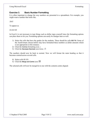
Below is a list of the icons available in the formatting toolbar along with a description of each.

Change the font style for the selected cells
Change the text size in the selected cells
Turns Bold formatting on and off in the selected cells [Ctrl] [B]
Turns Italic formatting on and off in the selected cells [Ctrl] [I]
Turns Underline formatting on and off in the selected cells [Ctrl] [U]
Aligns the contents of each of the selected cells to the left
Aligns the contents of each of the selected cells to the centre
Aligns the contents of each of the selected cells to the right
Merges the selected cells and aligns the contents to the centre
Formats the selected cells with the currency style ($#,###.##)
Formats the selected cells with the percent style (##%)
Formats the selected cells with the comma style (#,###.##)
Increases the number of decimal places
Decreases the number of decimal places
Decreases indent for the selected cells
Increases indent for the selected cells
Change the border style around the selected cells
Change the background colour of the selected cells
Change the colour of text in the selected cells



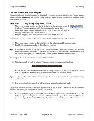
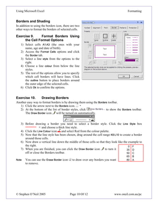
Exercise 2. Formatting Text in Individual Cells
1) Select cells A1:A3.
2) Click the Bold formatting icon or press [Ctrl] [B].

Note that clicking it again turns the bold formatting off.

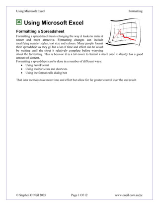
3) Click the arrow to the right of the Font Size box. A list of font (text) sizes will
appear as shown to the right.
4) Click 12. You can also type a number directly in the box and press [Enter] if the size you
want is not listed.

Note Font heights are measured in points. 72 points equals one inch.

5) Click the left align icon.
6) Click the arrow to the right of the font select box. A list of fonts will appear.
7) Type the letter C. The list will move to fonts with names that begin with C.
8) Click Comic Sans MS in the list to choose this font. You cal also type the font name in the
selection box and press [Enter].
9) Click the arrow next to the Font Colour icon. A list of available
font colours will appear as shown to the right.
10) From the list of colours, choose a colour and click it. You will notice
that the line on the bottom of the icon will turn to the colour you just
selected. You can choose that colour again by clicking on the icon
itself instead of clicking the arrow next to the icon.
11) Click the arrow next to the Font Colour icon again.

Notice the small horizontal lines above the word Automatic. This indicates that this colour palette
can be separated from the main toolbar.

12) Move your mouse over the horizontal lines. A caption should appear which says Drag to
make this menu float.
13) Drag downwards to turn this in to a floating menu. You can now select
colour without returning to the toolbar. When you have finished using
the colour palette, you can close it by clicking the cross icon in the
top-right corner. Floating menus like this can be found in other
icons and are common in other programs such as Word and
PowerPoint.

Note All of the formatting shortcuts we have used are identical to the ones
found in other programs such as Microsoft Word.

When your formatting is complete, the cells should look similar to the example below.



Exercise 3. Basic Number Formatting
It is often important to change the way numbers are presented in a spreadsheet. For example, you
might want a number that looks like.

3845

To appear as

$3,845.00

In Excel it is not necessary to type things such as dollar signs yourself since the formatting options
can place them in for you. Formatting options can easily be changes later as well.

1) Select the cells that have the grades for the students. These should be cells B6:F18. Some of
the AutoFormats chosen before may have formatted these numbers as dollar amounts which
is not appropriate in this instance.
2) Click the Comma formatting icon.
3) Click the Decrease Decimals icon twice.

The numbers should now be back to normal. Now we will format the main heading so that it
becomes centred across several cells.

4) Select cells B1:H1.
5) Click the Merge and Centre icon.

The selected cells will now be merged in to one with the contents centre aligned.



Column Widths and Row Heights
Column widths and Row heights can be adjusted by going to the menu and selecting Format, Column,
Width or Format, Row Height. It is usually easier, however, to do it using the mouse as demonstrated in
the following exercise.

Exercise 4. Adjusting Height And Width
1) Move your mouse pointer so that it is between the column A and B
headings. You mouse pointer will change to a double arrow shape.
2) Click your mouse button and drag to the right. A caption will appear
telling you how wide the column will be.
3) Keep on dragging until the column width reaches 15 (110 pixels).

You can also resize a column so that it will automatically fit the contents of the column.

4) Move your mouse pointer so that it is between the column A and B headings again.
5) Double-click to automatically fit the column’s contents.

Note: if you have a heading in the top of the column that is very wide then you may not want the
whole column to be that wide. If you want a column width to fit a selection of cells instead of
the entire column you can choose Format, Column, AutoFit Selection from the menu.

It is also possible to re-size several columns at the same time.

6) Select column B through to column F by dragging across the column headings.

7) Follow the first three steps in this exercise to change the width of any of the selected columns
to 9.29 (70 pixels). All of the selected columns will become the same width.

If you use the AutoFit method, then each column will resize to fit its contents so each column may
end up a different size.

8) Use any of the above methods to select suitable widths for columns G and H.

These same methods can also be used for adjusting the height of rows. Row height will often change
automatically when you change the size of text in the row.

Tip: If you want to have gaps in your table, instead of leaving rows and columns blank, it is often
better to adjust row heights and column widths to create the gaps. Some features of Excel can
automatically select an entire table, but only if there are no blank rows or columns.



Advanced Formatting Options
Many additional formatting options are not available on the Formatting Toolbar. These additional
options can be found in the Format Cells dialog as shown below.

There are six tabs along the top of the dialog box which allow you to go to different categories for
formatting. The first five tables will be demonstrated below. Sheet protection will be explained in a
later exercise.



Number Formats
Numbers, dollar amounts, percentages, dates and
times are all treated by Excel as numerical values.
As far as Excel is concerned, they are all numbers.
The only difference is the way they’re formatted.
In an earlier exercise, we used icons on the
toolbar so change the number format of the main
cells in the table. The toolbar icons only give a
few format choices. The Formatting options
however, give numerous number formatting
options and even allow you to create your own
custom number formats.

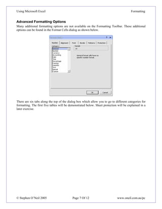
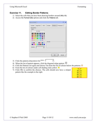
Exercise 5. Changing Number
Formats
1) Select the cells with the table averages
(B15:F15).
2) Access the Format Cells dialog box by using one of the following methods.
• From the menu, select Format, Cells.
• Right-click the selected cells and choose Format Cells.
• Press [Ctrl] [1].
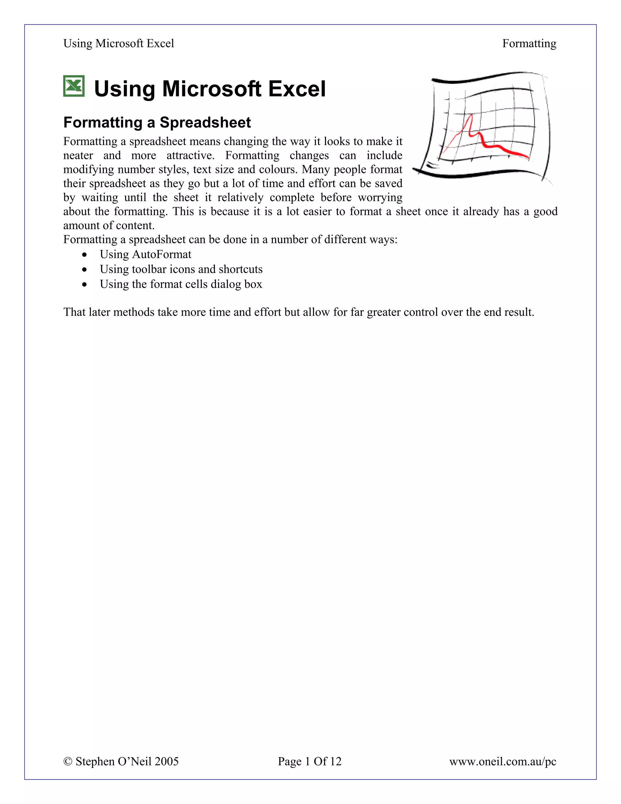
3) Make sure the Number tab is selected.
4) From the list of Categories on the left choose Number.
5) Set the number of Decimal Places to 2. Note that a sample of the selected number format
appears at the top.
6) Click OK to confirm the change.

Number formats will remain even if the numbers in the cells change.

Exercise 6. Changing Date Formats
1) Select cell A3.
2) Access the Format Cells options as shown above.
3) Choose Date for the number category.
4) Select a date format which includes the name of the month rather
than the number of the month.
5) Click Ok when done.

Note If you open the Format Numbers options and the only tab available is the Font tab, it is most
likely because you are editing the contents of a cell.



Text Formats
The next two Alignment and Font tabs are both
for the purpose of changing how the contents of
cells look.

Exercise 7. Aligning Text
1) Select the cells B5:H5.
2) Access the Format Cells options as shown
above.
3) Change the horizontal alignment to Left.
4) Change the Orientation to 45 Degrees (this
can be set by entering the number in the
degrees box shown or by dragging the
text line above it to the angle you want.
5) Click Ok to confirm the settings.
6) Select cell B1 (this cell should contain
your heading in the merged cells).
7) Access the Format Cells options.
8) Notice that the Merge Cells option is turned on and the Horizontal alignment is set to center
because we used the Merge and Center icon earlier. Click Cancel to leave these options as they
are.

Exercise 8. Font Options
1) Select cell B1.
2) Access the Format Cells options.
3) Select the Font tab.
4) Select the following options as shown to
the right:
• Font Style Bold
• Size 14
• Underline Double
• Colour Dark Blue
5) Click OK to confirm the changes.



Borders and Shading
In addition to using the borders icon, there are two
other ways to format the borders of selected cells.

Exercise 9. Format Borders Using
the Cell Format Options
1) Select cells A1:A3 (the ones with your
name, age and date of birth).
2) Access the Format Cells options and click
the Border tab.
3) Select a line style from the options to the
right.
4) Choose a line colour from below the line
styles.
5) The rest of the options allow you to specify
which cell borders will have lines. Click
the outline button to place borders around
the outer edge of the selected cells.
6) Click Ok to confirm the options.

Exercise 10. Drawing Borders
Another easy way to format borders is by drawing them using the Borders toolbar.
1) Click the arrow next to the Borders icon.
2) At the bottom of the list of border styles, click to show the Borders toolbar.
The Draw Border icon will be turned on automatically.

3) Before drawing a border you need to select a border style. Click the Line Style box
and choose a thick line style.
4) Click the Line Colour icon and select Red from the colour palette.
5) Now that the line style has been chosen, drag around the cell range K6:L10 to create a border
around those cells.
6) Now draw a vertical line down the middle of those cells so that they look like the example to
the right. 0 F
7) When you are finished, you can click the Draw Border icon to turn it 35 D
off or close the Borders toolbar. 50 C
65 B
Note You can use the Erase Border icon to draw over any borders you want 80 A
to remove.



Exercise 11. Editing Border Patterns
1) Select the cells that you have been drawing borders around (K6:L10).
2) Access the Format Cells options and click the Patterns tab.

3) Click the patterns drop-down list .
4) When the list of pattern appears, click the diagonal stripe pattern.
5) Click the Patterns list again and choose Tan from the list of colours below the patterns.
6) From the list of colours under cell shading click yellow.
0 F
7) Click OK to confirm the choices. The cells should now have a striped 35 D
pattern like the example to the right. 50 C
65 B
80 A



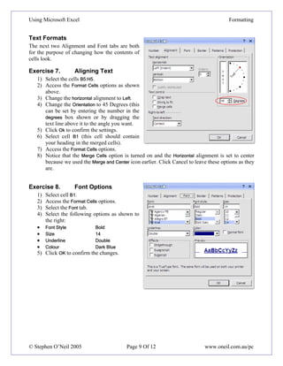
Exercise 12. Removing Formatting
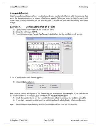
1) Click on a blank cell in your spreadsheet.
2) Click the Fill Colour icon to change the background colour of that cell.
3) Make sure that cell is still selected and press [Del].

Pressing delete will remove the contents of a cell but won’t affect the formatting in that cell. If you
want to remove formatting, such as the background colour in this cell, you need to use a different
method.

4) From the menu choose Edit, Clear, Formats.

All formatting will now be removed from that cell.

5) Save the changes to your Grades worksheet.

Note If you enter text or numbers in to a blank cell and get unexpected results, it is often because
of some text or number formatting left over from something that was previously in those
cells.


Using Microsoft Excel3 Formatting

Recommended

Recommended

More Related Content

What's hot

What's hot (19)

Similar to Using Microsoft Excel3 Formatting

Similar to Using Microsoft Excel3 Formatting (20)

More from Jack Frost

More from Jack Frost (20)

Recently uploaded

Recently uploaded (20)

Using Microsoft Excel3 Formatting