Download as PDF, PPTX


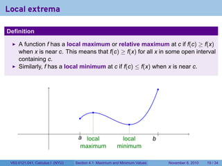
![The Extreme Value Theorem
Theorem (The Extreme Value Theorem)
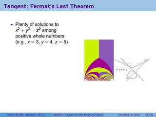
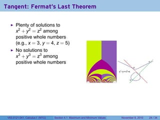
Let f be a function which is continuous on the closed interval [a, b].
Then f attains an absolute maximum value f(c) and an absolute
minimum value f(d) at numbers c and d in [a, b].
V63.0121.041, Calculus I (NYU) Section 4.1 Maximum and Minimum Values November 8, 2010 13 / 34](https://image.slidesharecdn.com/lesson18-maximumandminimumvalues041slides-101108142857-phpapp02-121002220407-phpapp02/85/Lesson-18-Maximum-and-Minimum-Values-Section-041-slides-16-320.jpg)
![The Extreme Value Theorem
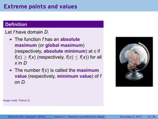
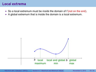
Theorem (The Extreme Value Theorem)
Let f be a function which is continuous on the closed interval [a, b].
Then f attains an absolute maximum value f(c) and an absolute
minimum value f(d) at numbers c and d in [a, b].
.
.
. .
a
. b
.
V63.0121.041, Calculus I (NYU) Section 4.1 Maximum and Minimum Values November 8, 2010 13 / 34](https://image.slidesharecdn.com/lesson18-maximumandminimumvalues041slides-101108142857-phpapp02-121002220407-phpapp02/85/Lesson-18-Maximum-and-Minimum-Values-Section-041-slides-17-320.jpg)
![The Extreme Value Theorem
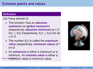
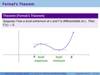
Theorem (The Extreme Value Theorem)
Let f be a function which is continuous on the closed interval [a, b].
Then f attains an absolute maximum value f(c) and an absolute
minimum value f(d) at numbers c and d in [a, b].
.
maximum .(c)
f
.
value
. .
minimum .(d)
f
.
value
. . ..
a
. d c
b
.
minimum maximum
V63.0121.041, Calculus I (NYU) Section 4.1 Maximum and Minimum Values November 8, 2010 13 / 34](https://image.slidesharecdn.com/lesson18-maximumandminimumvalues041slides-101108142857-phpapp02-121002220407-phpapp02/85/Lesson-18-Maximum-and-Minimum-Values-Section-041-slides-18-320.jpg)
![Bad Example #1
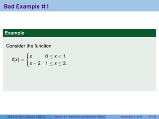
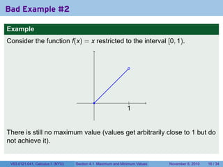
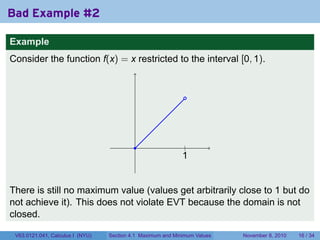
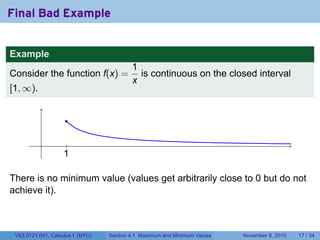
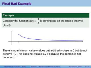
Example
Consider the function .
{
x 0≤x<1
f(x) = . .
| .
x − 2 1 ≤ x ≤ 2. 1
.
.
Then although values of f(x) get arbitrarily close to 1 and never bigger
than 1, 1 is not the maximum value of f on [0, 1] because it is never
achieved.
V63.0121.041, Calculus I (NYU) Section 4.1 Maximum and Minimum Values November 8, 2010 15 / 34](https://image.slidesharecdn.com/lesson18-maximumandminimumvalues041slides-101108142857-phpapp02-121002220407-phpapp02/85/Lesson-18-Maximum-and-Minimum-Values-Section-041-slides-22-320.jpg)
![Bad Example #1
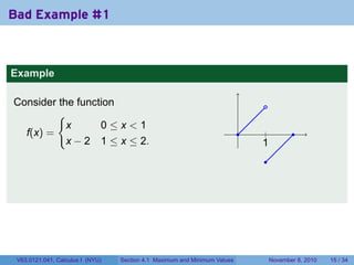
Example
Consider the function .
{
x 0≤x<1
f(x) = . .
| .
x − 2 1 ≤ x ≤ 2. 1
.
.
Then although values of f(x) get arbitrarily close to 1 and never bigger
than 1, 1 is not the maximum value of f on [0, 1] because it is never
achieved. This does not violate EVT because f is not continuous.
V63.0121.041, Calculus I (NYU) Section 4.1 Maximum and Minimum Values November 8, 2010 15 / 34](https://image.slidesharecdn.com/lesson18-maximumandminimumvalues041slides-101108142857-phpapp02-121002220407-phpapp02/85/Lesson-18-Maximum-and-Minimum-Values-Section-041-slides-23-320.jpg)


![Flowchart for placing extrema
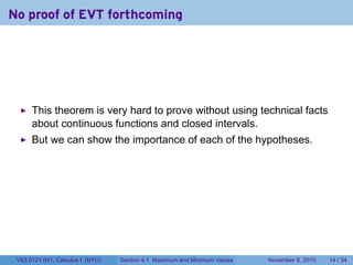
Thanks to Fermat
Suppose f is a continuous function on the closed, bounded interval
[a, b], and c is a global maximum point.
.
. . c is a
start
local max
. . .
Is c an Is f diff’ble f is not
n
.o n
.o
endpoint? at c? diff at c
y
. es y
. es
. .
c = a or
f′ (c) = 0
c = b
V63.0121.041, Calculus I (NYU) Section 4.1 Maximum and Minimum Values November 8, 2010 26 / 34](https://image.slidesharecdn.com/lesson18-maximumandminimumvalues041slides-101108142857-phpapp02-121002220407-phpapp02/85/Lesson-18-Maximum-and-Minimum-Values-Section-041-slides-50-320.jpg)
![The Closed Interval Method
This means to find the maximum value of f on [a, b], we need to:
Evaluate f at the endpoints a and b
Evaluate f at the critical points or critical numbers x where
either f′ (x) = 0 or f is not differentiable at x.
The points with the largest function value are the global maximum
points
The points with the smallest or most negative function value are
the global minimum points.
V63.0121.041, Calculus I (NYU) Section 4.1 Maximum and Minimum Values November 8, 2010 27 / 34](https://image.slidesharecdn.com/lesson18-maximumandminimumvalues041slides-101108142857-phpapp02-121002220407-phpapp02/85/Lesson-18-Maximum-and-Minimum-Values-Section-041-slides-51-320.jpg)
![Extreme values of a linear function
Example
Find the extreme values of f(x) = 2x − 5 on [−1, 2].
V63.0121.041, Calculus I (NYU) Section 4.1 Maximum and Minimum Values November 8, 2010 29 / 34](https://image.slidesharecdn.com/lesson18-maximumandminimumvalues041slides-101108142857-phpapp02-121002220407-phpapp02/85/Lesson-18-Maximum-and-Minimum-Values-Section-041-slides-53-320.jpg)
![Extreme values of a linear function
Example
Find the extreme values of f(x) = 2x − 5 on [−1, 2].
Solution
Since f′ (x) = 2, which is never zero, we have no critical points and we
need only investigate the endpoints:
f(−1) = 2(−1) − 5 = −7
f(2) = 2(2) − 5 = −1
V63.0121.041, Calculus I (NYU) Section 4.1 Maximum and Minimum Values November 8, 2010 29 / 34](https://image.slidesharecdn.com/lesson18-maximumandminimumvalues041slides-101108142857-phpapp02-121002220407-phpapp02/85/Lesson-18-Maximum-and-Minimum-Values-Section-041-slides-54-320.jpg)
![Extreme values of a linear function
Example
Find the extreme values of f(x) = 2x − 5 on [−1, 2].
Solution
Since f′ (x) = 2, which is never zero, we have no critical points and we
need only investigate the endpoints:
f(−1) = 2(−1) − 5 = −7
f(2) = 2(2) − 5 = −1
So
The absolute minimum (point) is at −1; the minimum value is −7.
The absolute maximum (point) is at 2; the maximum value is −1.
V63.0121.041, Calculus I (NYU) Section 4.1 Maximum and Minimum Values November 8, 2010 29 / 34](https://image.slidesharecdn.com/lesson18-maximumandminimumvalues041slides-101108142857-phpapp02-121002220407-phpapp02/85/Lesson-18-Maximum-and-Minimum-Values-Section-041-slides-55-320.jpg)
![Extreme values of a quadratic function
Example
Find the extreme values of f(x) = x2 − 1 on [−1, 2].
V63.0121.041, Calculus I (NYU) Section 4.1 Maximum and Minimum Values November 8, 2010 30 / 34](https://image.slidesharecdn.com/lesson18-maximumandminimumvalues041slides-101108142857-phpapp02-121002220407-phpapp02/85/Lesson-18-Maximum-and-Minimum-Values-Section-041-slides-56-320.jpg)
![Extreme values of a quadratic function
Example
Find the extreme values of f(x) = x2 − 1 on [−1, 2].
Solution
We have f′ (x) = 2x, which is zero when x = 0.
V63.0121.041, Calculus I (NYU) Section 4.1 Maximum and Minimum Values November 8, 2010 30 / 34](https://image.slidesharecdn.com/lesson18-maximumandminimumvalues041slides-101108142857-phpapp02-121002220407-phpapp02/85/Lesson-18-Maximum-and-Minimum-Values-Section-041-slides-57-320.jpg)
![Extreme values of a quadratic function
Example
Find the extreme values of f(x) = x2 − 1 on [−1, 2].
Solution
We have f′ (x) = 2x, which is zero when x = 0. So our points to check
are:
f(−1) =
f(0) =
f(2) =
V63.0121.041, Calculus I (NYU) Section 4.1 Maximum and Minimum Values November 8, 2010 30 / 34](https://image.slidesharecdn.com/lesson18-maximumandminimumvalues041slides-101108142857-phpapp02-121002220407-phpapp02/85/Lesson-18-Maximum-and-Minimum-Values-Section-041-slides-58-320.jpg)
![Extreme values of a quadratic function
Example
Find the extreme values of f(x) = x2 − 1 on [−1, 2].
Solution
We have f′ (x) = 2x, which is zero when x = 0. So our points to check
are:
f(−1) = 0
f(0) =
f(2) =
V63.0121.041, Calculus I (NYU) Section 4.1 Maximum and Minimum Values November 8, 2010 30 / 34](https://image.slidesharecdn.com/lesson18-maximumandminimumvalues041slides-101108142857-phpapp02-121002220407-phpapp02/85/Lesson-18-Maximum-and-Minimum-Values-Section-041-slides-59-320.jpg)
![Extreme values of a quadratic function
Example
Find the extreme values of f(x) = x2 − 1 on [−1, 2].
Solution
We have f′ (x) = 2x, which is zero when x = 0. So our points to check
are:
f(−1) = 0
f(0) = − 1
f(2) =
V63.0121.041, Calculus I (NYU) Section 4.1 Maximum and Minimum Values November 8, 2010 30 / 34](https://image.slidesharecdn.com/lesson18-maximumandminimumvalues041slides-101108142857-phpapp02-121002220407-phpapp02/85/Lesson-18-Maximum-and-Minimum-Values-Section-041-slides-60-320.jpg)
![Extreme values of a quadratic function
Example
Find the extreme values of f(x) = x2 − 1 on [−1, 2].
Solution
We have f′ (x) = 2x, which is zero when x = 0. So our points to check
are:
f(−1) = 0
f(0) = − 1
f(2) = 3
V63.0121.041, Calculus I (NYU) Section 4.1 Maximum and Minimum Values November 8, 2010 30 / 34](https://image.slidesharecdn.com/lesson18-maximumandminimumvalues041slides-101108142857-phpapp02-121002220407-phpapp02/85/Lesson-18-Maximum-and-Minimum-Values-Section-041-slides-61-320.jpg)
![Extreme values of a quadratic function
Example
Find the extreme values of f(x) = x2 − 1 on [−1, 2].
Solution
We have f′ (x) = 2x, which is zero when x = 0. So our points to check
are:
f(−1) = 0
f(0) = − 1 (absolute min)
f(2) = 3
V63.0121.041, Calculus I (NYU) Section 4.1 Maximum and Minimum Values November 8, 2010 30 / 34](https://image.slidesharecdn.com/lesson18-maximumandminimumvalues041slides-101108142857-phpapp02-121002220407-phpapp02/85/Lesson-18-Maximum-and-Minimum-Values-Section-041-slides-62-320.jpg)
![Extreme values of a quadratic function
Example
Find the extreme values of f(x) = x2 − 1 on [−1, 2].
Solution
We have f′ (x) = 2x, which is zero when x = 0. So our points to check
are:
f(−1) = 0
f(0) = − 1 (absolute min)
f(2) = 3 (absolute max)
V63.0121.041, Calculus I (NYU) Section 4.1 Maximum and Minimum Values November 8, 2010 30 / 34](https://image.slidesharecdn.com/lesson18-maximumandminimumvalues041slides-101108142857-phpapp02-121002220407-phpapp02/85/Lesson-18-Maximum-and-Minimum-Values-Section-041-slides-63-320.jpg)
![Extreme values of a cubic function
Example
Find the extreme values of f(x) = 2x3 − 3x2 + 1 on [−1, 2].
V63.0121.041, Calculus I (NYU) Section 4.1 Maximum and Minimum Values November 8, 2010 31 / 34](https://image.slidesharecdn.com/lesson18-maximumandminimumvalues041slides-101108142857-phpapp02-121002220407-phpapp02/85/Lesson-18-Maximum-and-Minimum-Values-Section-041-slides-64-320.jpg)
![Extreme values of a cubic function
Example
Find the extreme values of f(x) = 2x3 − 3x2 + 1 on [−1, 2].
Solution
Since f′ (x) = 6x2 − 6x = 6x(x − 1), we have critical points at x = 0 and
x = 1.
V63.0121.041, Calculus I (NYU) Section 4.1 Maximum and Minimum Values November 8, 2010 31 / 34](https://image.slidesharecdn.com/lesson18-maximumandminimumvalues041slides-101108142857-phpapp02-121002220407-phpapp02/85/Lesson-18-Maximum-and-Minimum-Values-Section-041-slides-65-320.jpg)
![Extreme values of a cubic function
Example
Find the extreme values of f(x) = 2x3 − 3x2 + 1 on [−1, 2].
Solution
Since f′ (x) = 6x2 − 6x = 6x(x − 1), we have critical points at x = 0 and
x = 1. The values to check are
V63.0121.041, Calculus I (NYU) Section 4.1 Maximum and Minimum Values November 8, 2010 31 / 34](https://image.slidesharecdn.com/lesson18-maximumandminimumvalues041slides-101108142857-phpapp02-121002220407-phpapp02/85/Lesson-18-Maximum-and-Minimum-Values-Section-041-slides-66-320.jpg)
![Extreme values of a cubic function
Example
Find the extreme values of f(x) = 2x3 − 3x2 + 1 on [−1, 2].
Solution
Since f′ (x) = 6x2 − 6x = 6x(x − 1), we have critical points at x = 0 and
x = 1. The values to check are
f(−1) = − 4
V63.0121.041, Calculus I (NYU) Section 4.1 Maximum and Minimum Values November 8, 2010 31 / 34](https://image.slidesharecdn.com/lesson18-maximumandminimumvalues041slides-101108142857-phpapp02-121002220407-phpapp02/85/Lesson-18-Maximum-and-Minimum-Values-Section-041-slides-67-320.jpg)
![Extreme values of a cubic function
Example
Find the extreme values of f(x) = 2x3 − 3x2 + 1 on [−1, 2].
Solution
Since f′ (x) = 6x2 − 6x = 6x(x − 1), we have critical points at x = 0 and
x = 1. The values to check are
f(−1) = − 4
f(0) = 1
V63.0121.041, Calculus I (NYU) Section 4.1 Maximum and Minimum Values November 8, 2010 31 / 34](https://image.slidesharecdn.com/lesson18-maximumandminimumvalues041slides-101108142857-phpapp02-121002220407-phpapp02/85/Lesson-18-Maximum-and-Minimum-Values-Section-041-slides-68-320.jpg)
![Extreme values of a cubic function
Example
Find the extreme values of f(x) = 2x3 − 3x2 + 1 on [−1, 2].
Solution
Since f′ (x) = 6x2 − 6x = 6x(x − 1), we have critical points at x = 0 and
x = 1. The values to check are
f(−1) = − 4
f(0) = 1
f(1) = 0
V63.0121.041, Calculus I (NYU) Section 4.1 Maximum and Minimum Values November 8, 2010 31 / 34](https://image.slidesharecdn.com/lesson18-maximumandminimumvalues041slides-101108142857-phpapp02-121002220407-phpapp02/85/Lesson-18-Maximum-and-Minimum-Values-Section-041-slides-69-320.jpg)
![Extreme values of a cubic function
Example
Find the extreme values of f(x) = 2x3 − 3x2 + 1 on [−1, 2].
Solution
Since f′ (x) = 6x2 − 6x = 6x(x − 1), we have critical points at x = 0 and
x = 1. The values to check are
f(−1) = − 4
f(0) = 1
f(1) = 0
f(2) = 5
V63.0121.041, Calculus I (NYU) Section 4.1 Maximum and Minimum Values November 8, 2010 31 / 34](https://image.slidesharecdn.com/lesson18-maximumandminimumvalues041slides-101108142857-phpapp02-121002220407-phpapp02/85/Lesson-18-Maximum-and-Minimum-Values-Section-041-slides-70-320.jpg)
![Extreme values of a cubic function
Example
Find the extreme values of f(x) = 2x3 − 3x2 + 1 on [−1, 2].
Solution
Since f′ (x) = 6x2 − 6x = 6x(x − 1), we have critical points at x = 0 and
x = 1. The values to check are
f(−1) = − 4 (global min)
f(0) = 1
f(1) = 0
f(2) = 5
V63.0121.041, Calculus I (NYU) Section 4.1 Maximum and Minimum Values November 8, 2010 31 / 34](https://image.slidesharecdn.com/lesson18-maximumandminimumvalues041slides-101108142857-phpapp02-121002220407-phpapp02/85/Lesson-18-Maximum-and-Minimum-Values-Section-041-slides-71-320.jpg)
![Extreme values of a cubic function
Example
Find the extreme values of f(x) = 2x3 − 3x2 + 1 on [−1, 2].
Solution
Since f′ (x) = 6x2 − 6x = 6x(x − 1), we have critical points at x = 0 and
x = 1. The values to check are
f(−1) = − 4 (global min)
f(0) = 1
f(1) = 0
f(2) = 5 (global max)
V63.0121.041, Calculus I (NYU) Section 4.1 Maximum and Minimum Values November 8, 2010 31 / 34](https://image.slidesharecdn.com/lesson18-maximumandminimumvalues041slides-101108142857-phpapp02-121002220407-phpapp02/85/Lesson-18-Maximum-and-Minimum-Values-Section-041-slides-72-320.jpg)
![Extreme values of a cubic function
Example
Find the extreme values of f(x) = 2x3 − 3x2 + 1 on [−1, 2].
Solution
Since f′ (x) = 6x2 − 6x = 6x(x − 1), we have critical points at x = 0 and
x = 1. The values to check are
f(−1) = − 4 (global min)
f(0) = 1 (local max)
f(1) = 0
f(2) = 5 (global max)
V63.0121.041, Calculus I (NYU) Section 4.1 Maximum and Minimum Values November 8, 2010 31 / 34](https://image.slidesharecdn.com/lesson18-maximumandminimumvalues041slides-101108142857-phpapp02-121002220407-phpapp02/85/Lesson-18-Maximum-and-Minimum-Values-Section-041-slides-73-320.jpg)
![Extreme values of a cubic function
Example
Find the extreme values of f(x) = 2x3 − 3x2 + 1 on [−1, 2].
Solution
Since f′ (x) = 6x2 − 6x = 6x(x − 1), we have critical points at x = 0 and
x = 1. The values to check are
f(−1) = − 4 (global min)
f(0) = 1 (local max)
f(1) = 0 (local min)
f(2) = 5 (global max)
V63.0121.041, Calculus I (NYU) Section 4.1 Maximum and Minimum Values November 8, 2010 31 / 34](https://image.slidesharecdn.com/lesson18-maximumandminimumvalues041slides-101108142857-phpapp02-121002220407-phpapp02/85/Lesson-18-Maximum-and-Minimum-Values-Section-041-slides-74-320.jpg)
![Extreme values of an algebraic function
Example
Find the extreme values of f(x) = x2/3 (x + 2) on [−1, 2].
V63.0121.041, Calculus I (NYU) Section 4.1 Maximum and Minimum Values November 8, 2010 32 / 34](https://image.slidesharecdn.com/lesson18-maximumandminimumvalues041slides-101108142857-phpapp02-121002220407-phpapp02/85/Lesson-18-Maximum-and-Minimum-Values-Section-041-slides-75-320.jpg)
![Extreme values of an algebraic function
Example
Find the extreme values of f(x) = x2/3 (x + 2) on [−1, 2].
Solution
Write f(x) = x5/3 + 2x2/3 , then
5 2/3 4 −1/3 1 −1/3
f′ (x) = x + x = x (5x + 4)
3 3 3
Thus f′ (−4/5) = 0 and f is not differentiable at 0.
V63.0121.041, Calculus I (NYU) Section 4.1 Maximum and Minimum Values November 8, 2010 32 / 34](https://image.slidesharecdn.com/lesson18-maximumandminimumvalues041slides-101108142857-phpapp02-121002220407-phpapp02/85/Lesson-18-Maximum-and-Minimum-Values-Section-041-slides-76-320.jpg)
![Extreme values of an algebraic function
Example
Find the extreme values of f(x) = x2/3 (x + 2) on [−1, 2].
Solution
Write f(x) = x5/3 + 2x2/3 , then
5 2/3 4 −1/3 1 −1/3
f′ (x) = x + x = x (5x + 4)
3 3 3
Thus f′ (−4/5) = 0 and f is not differentiable at 0. So our points to
check are:
f(−1) =
V63.0121.041, Calculus I (NYU) Section 4.1 Maximum and Minimum Values November 8, 2010 32 / 34](https://image.slidesharecdn.com/lesson18-maximumandminimumvalues041slides-101108142857-phpapp02-121002220407-phpapp02/85/Lesson-18-Maximum-and-Minimum-Values-Section-041-slides-77-320.jpg)
![Extreme values of an algebraic function
Example
Find the extreme values of f(x) = x2/3 (x + 2) on [−1, 2].
Solution
Write f(x) = x5/3 + 2x2/3 , then
5 2/3 4 −1/3 1 −1/3
f′ (x) = x + x = x (5x + 4)
3 3 3
Thus f′ (−4/5) = 0 and f is not differentiable at 0. So our points to
check are:
f(−1) = 1
f(−4/5) =
V63.0121.041, Calculus I (NYU) Section 4.1 Maximum and Minimum Values November 8, 2010 32 / 34](https://image.slidesharecdn.com/lesson18-maximumandminimumvalues041slides-101108142857-phpapp02-121002220407-phpapp02/85/Lesson-18-Maximum-and-Minimum-Values-Section-041-slides-78-320.jpg)
![Extreme values of an algebraic function
Example
Find the extreme values of f(x) = x2/3 (x + 2) on [−1, 2].
Solution
Write f(x) = x5/3 + 2x2/3 , then
5 2/3 4 −1/3 1 −1/3
f′ (x) = x + x = x (5x + 4)
3 3 3
Thus f′ (−4/5) = 0 and f is not differentiable at 0. So our points to
check are:
f(−1) = 1
f(−4/5) = 1.0341
f(0) =
V63.0121.041, Calculus I (NYU) Section 4.1 Maximum and Minimum Values November 8, 2010 32 / 34](https://image.slidesharecdn.com/lesson18-maximumandminimumvalues041slides-101108142857-phpapp02-121002220407-phpapp02/85/Lesson-18-Maximum-and-Minimum-Values-Section-041-slides-79-320.jpg)
![Extreme values of an algebraic function
Example
Find the extreme values of f(x) = x2/3 (x + 2) on [−1, 2].
Solution
Write f(x) = x5/3 + 2x2/3 , then
5 2/3 4 −1/3 1 −1/3
f′ (x) = x + x = x (5x + 4)
3 3 3
Thus f′ (−4/5) = 0 and f is not differentiable at 0. So our points to
check are:
f(−1) = 1
f(−4/5) = 1.0341
f(0) = 0
f(2) =
V63.0121.041, Calculus I (NYU) Section 4.1 Maximum and Minimum Values November 8, 2010 32 / 34](https://image.slidesharecdn.com/lesson18-maximumandminimumvalues041slides-101108142857-phpapp02-121002220407-phpapp02/85/Lesson-18-Maximum-and-Minimum-Values-Section-041-slides-80-320.jpg)
![Extreme values of an algebraic function
Example
Find the extreme values of f(x) = x2/3 (x + 2) on [−1, 2].
Solution
Write f(x) = x5/3 + 2x2/3 , then
5 2/3 4 −1/3 1 −1/3
f′ (x) = x + x = x (5x + 4)
3 3 3
Thus f′ (−4/5) = 0 and f is not differentiable at 0. So our points to
check are:
f(−1) = 1
f(−4/5) = 1.0341
f(0) = 0
f(2) = 6.3496
V63.0121.041, Calculus I (NYU) Section 4.1 Maximum and Minimum Values November 8, 2010 32 / 34](https://image.slidesharecdn.com/lesson18-maximumandminimumvalues041slides-101108142857-phpapp02-121002220407-phpapp02/85/Lesson-18-Maximum-and-Minimum-Values-Section-041-slides-81-320.jpg)
![Extreme values of an algebraic function
Example
Find the extreme values of f(x) = x2/3 (x + 2) on [−1, 2].
Solution
Write f(x) = x5/3 + 2x2/3 , then
5 2/3 4 −1/3 1 −1/3
f′ (x) = x + x = x (5x + 4)
3 3 3
Thus f′ (−4/5) = 0 and f is not differentiable at 0. So our points to
check are:
f(−1) = 1
f(−4/5) = 1.0341
f(0) = 0 (absolute min)
f(2) = 6.3496
V63.0121.041, Calculus I (NYU) Section 4.1 Maximum and Minimum Values November 8, 2010 32 / 34](https://image.slidesharecdn.com/lesson18-maximumandminimumvalues041slides-101108142857-phpapp02-121002220407-phpapp02/85/Lesson-18-Maximum-and-Minimum-Values-Section-041-slides-82-320.jpg)
![Extreme values of an algebraic function
Example
Find the extreme values of f(x) = x2/3 (x + 2) on [−1, 2].
Solution
Write f(x) = x5/3 + 2x2/3 , then
5 2/3 4 −1/3 1 −1/3
f′ (x) = x + x = x (5x + 4)
3 3 3
Thus f′ (−4/5) = 0 and f is not differentiable at 0. So our points to
check are:
f(−1) = 1
f(−4/5) = 1.0341
f(0) = 0 (absolute min)
f(2) = 6.3496 (absolute max)
V63.0121.041, Calculus I (NYU) Section 4.1 Maximum and Minimum Values November 8, 2010 32 / 34](https://image.slidesharecdn.com/lesson18-maximumandminimumvalues041slides-101108142857-phpapp02-121002220407-phpapp02/85/Lesson-18-Maximum-and-Minimum-Values-Section-041-slides-83-320.jpg)
![Extreme values of an algebraic function
Example
Find the extreme values of f(x) = x2/3 (x + 2) on [−1, 2].
Solution
Write f(x) = x5/3 + 2x2/3 , then
5 2/3 4 −1/3 1 −1/3
f′ (x) = x + x = x (5x + 4)
3 3 3
Thus f′ (−4/5) = 0 and f is not differentiable at 0. So our points to
check are:
f(−1) = 1
f(−4/5) = 1.0341 (relative max)
f(0) = 0 (absolute min)
f(2) = 6.3496 (absolute max)
V63.0121.041, Calculus I (NYU) Section 4.1 Maximum and Minimum Values November 8, 2010 32 / 34](https://image.slidesharecdn.com/lesson18-maximumandminimumvalues041slides-101108142857-phpapp02-121002220407-phpapp02/85/Lesson-18-Maximum-and-Minimum-Values-Section-041-slides-84-320.jpg)
![Extreme values of another algebraic function
Example
√
Find the extreme values of f(x) = 4 − x2 on [−2, 1].
V63.0121.041, Calculus I (NYU) Section 4.1 Maximum and Minimum Values November 8, 2010 33 / 34](https://image.slidesharecdn.com/lesson18-maximumandminimumvalues041slides-101108142857-phpapp02-121002220407-phpapp02/85/Lesson-18-Maximum-and-Minimum-Values-Section-041-slides-85-320.jpg)
![Extreme values of another algebraic function
Example
√
Find the extreme values of f(x) = 4 − x2 on [−2, 1].
Solution
x
We have f′ (x) = − √ , which is zero when x = 0. (f is not
4 − x2
differentiable at ±2 as well.)
V63.0121.041, Calculus I (NYU) Section 4.1 Maximum and Minimum Values November 8, 2010 33 / 34](https://image.slidesharecdn.com/lesson18-maximumandminimumvalues041slides-101108142857-phpapp02-121002220407-phpapp02/85/Lesson-18-Maximum-and-Minimum-Values-Section-041-slides-86-320.jpg)
![Extreme values of another algebraic function
Example
√
Find the extreme values of f(x) = 4 − x2 on [−2, 1].
Solution
x
We have f′ (x) = − √ , which is zero when x = 0. (f is not
4 − x2
differentiable at ±2 as well.) So our points to check are:
f(−2) =
V63.0121.041, Calculus I (NYU) Section 4.1 Maximum and Minimum Values November 8, 2010 33 / 34](https://image.slidesharecdn.com/lesson18-maximumandminimumvalues041slides-101108142857-phpapp02-121002220407-phpapp02/85/Lesson-18-Maximum-and-Minimum-Values-Section-041-slides-87-320.jpg)
![Extreme values of another algebraic function
Example
√
Find the extreme values of f(x) = 4 − x2 on [−2, 1].
Solution
x
We have f′ (x) = − √ , which is zero when x = 0. (f is not
4 − x2
differentiable at ±2 as well.) So our points to check are:
f(−2) = 0
f(0) =
V63.0121.041, Calculus I (NYU) Section 4.1 Maximum and Minimum Values November 8, 2010 33 / 34](https://image.slidesharecdn.com/lesson18-maximumandminimumvalues041slides-101108142857-phpapp02-121002220407-phpapp02/85/Lesson-18-Maximum-and-Minimum-Values-Section-041-slides-88-320.jpg)
![Extreme values of another algebraic function
Example
√
Find the extreme values of f(x) = 4 − x2 on [−2, 1].
Solution
x
We have f′ (x) = − √ , which is zero when x = 0. (f is not
4 − x2
differentiable at ±2 as well.) So our points to check are:
f(−2) = 0
f(0) = 2
f(1) =
V63.0121.041, Calculus I (NYU) Section 4.1 Maximum and Minimum Values November 8, 2010 33 / 34](https://image.slidesharecdn.com/lesson18-maximumandminimumvalues041slides-101108142857-phpapp02-121002220407-phpapp02/85/Lesson-18-Maximum-and-Minimum-Values-Section-041-slides-89-320.jpg)
![Extreme values of another algebraic function
Example
√
Find the extreme values of f(x) = 4 − x2 on [−2, 1].
Solution
x
We have f′ (x) = − √ , which is zero when x = 0. (f is not
4 − x2
differentiable at ±2 as well.) So our points to check are:
f(−2) = 0
f(0) = 2
√
f(1) = 3
V63.0121.041, Calculus I (NYU) Section 4.1 Maximum and Minimum Values November 8, 2010 33 / 34](https://image.slidesharecdn.com/lesson18-maximumandminimumvalues041slides-101108142857-phpapp02-121002220407-phpapp02/85/Lesson-18-Maximum-and-Minimum-Values-Section-041-slides-90-320.jpg)
![Extreme values of another algebraic function
Example
√
Find the extreme values of f(x) = 4 − x2 on [−2, 1].
Solution
x
We have f′ (x) = − √ , which is zero when x = 0. (f is not
4 − x2
differentiable at ±2 as well.) So our points to check are:
f(−2) = 0 (absolute min)
f(0) = 2
√
f(1) = 3
V63.0121.041, Calculus I (NYU) Section 4.1 Maximum and Minimum Values November 8, 2010 33 / 34](https://image.slidesharecdn.com/lesson18-maximumandminimumvalues041slides-101108142857-phpapp02-121002220407-phpapp02/85/Lesson-18-Maximum-and-Minimum-Values-Section-041-slides-91-320.jpg)
![Extreme values of another algebraic function
Example
√
Find the extreme values of f(x) = 4 − x2 on [−2, 1].
Solution
x
We have f′ (x) = − √ , which is zero when x = 0. (f is not
4 − x2
differentiable at ±2 as well.) So our points to check are:
f(−2) = 0 (absolute min)
f(0) = 2 (absolute max)
√
f(1) = 3
V63.0121.041, Calculus I (NYU) Section 4.1 Maximum and Minimum Values November 8, 2010 33 / 34](https://image.slidesharecdn.com/lesson18-maximumandminimumvalues041slides-101108142857-phpapp02-121002220407-phpapp02/85/Lesson-18-Maximum-and-Minimum-Values-Section-041-slides-92-320.jpg)

The document is a lecture note for a Calculus I course at New York University, focusing on maximum and minimum values, including concepts such as the extreme value theorem and Fermat's theorem. It outlines methods for finding extreme values of functions on closed intervals and discusses the significance of these values in optimization. The document also provides examples of continuous functions, illustrating cases where extreme values are achieved or not.