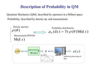
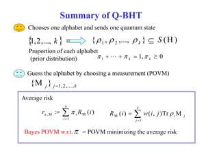
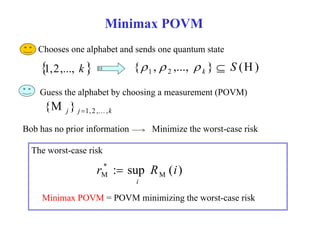
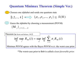
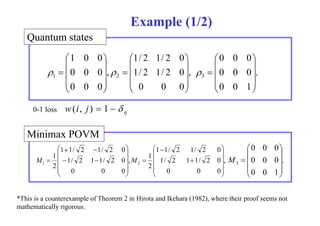
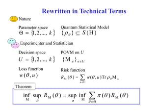
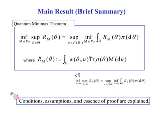
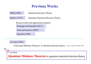
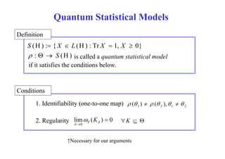
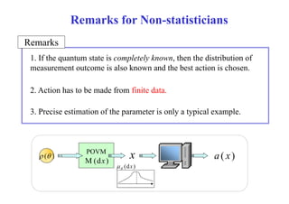
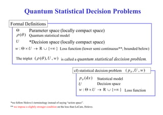
This document presents a presentation on the quantum minimax theorem in statistical decision theory, focusing on Bayesian statistics and its differences from traditional frequentist statistics. The discussion outlines the roles of prior distributions, statistical models, and measurement techniques within quantum mechanics, and proposes a framework for quantum Bayesian hypothesis testing. It concludes with a detailed overview of the quantum minimax theorem and its implications for optimal decision-making under uncertainty.
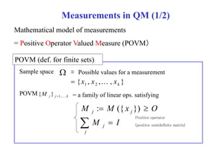

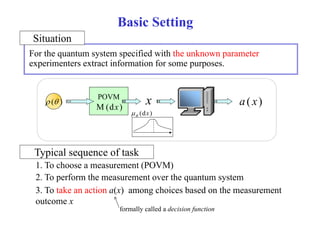
![Decision Functions
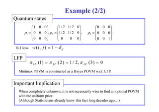
Example
- Estimate the unknown parameter x 1
a ( x )
xn n
x) - Estimate the unknown d.o. rather than parameter
a ( x ) a ( x
) 0
1 2
( ) ( ) 0
0 0 1 ( ) ( )
1 3
3
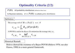
*
2
a x a x
a x a x
- Validate the entanglement/separability a ( x ) 0,1
- Constr ct Construct confidence region (credible region)
[a L (x), a R
(x)]](https://image.slidesharecdn.com/slide2014rims1031public-141101055906-conversion-gate02/85/Quantum-Minimax-Theorem-in-Statistical-Decision-Theory-RIMS2014-34-320.jpg)
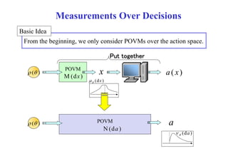
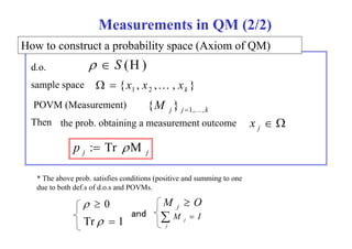
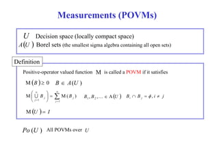
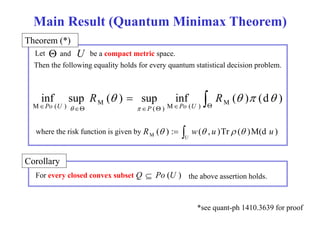
![Comparison of POVMs
The loss (e.g. squared error) depends on both unknown parameter
and
our decision u u, which is a random variable variable.( (u ~ (du )
Tr ( )M(du ) )
In order to compare two POVMs, we focus on the average of the loss
w w.r r.t t. the distribution of u
u.
( ) POVM
E[w( , u )]
u
(du )
M(du )
N(du ' )
Compared at the same
POVM E'[w( ,u')]
( ) u '
(du ' ) ](https://image.slidesharecdn.com/slide2014rims1031public-141101055906-conversion-gate02/85/Quantum-Minimax-Theorem-in-Statistical-Decision-Theory-RIMS2014-40-320.jpg)
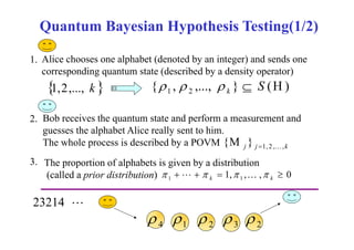
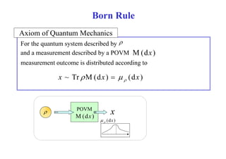
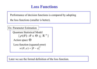
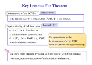
![Ex. of Loss Functions and Risk Functions
Parameter Estimation
{ ( ) : R m }
U 2 w( , u ) u
R ( ) u Tr ( )M(d u ) 2
M E [ ] 2 u
U
Construction of Predictive Density Operator
{ ( ) n : R p }
U S (H m ) w( , u ) D ( ( ) m || u )
R ( ) D( ( ) m || u )Tr ( ) m M(d u ) M U](https://image.slidesharecdn.com/slide2014rims1031public-141101055906-conversion-gate02/85/Quantum-Minimax-Theorem-in-Statistical-Decision-Theory-RIMS2014-44-320.jpg)

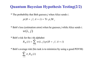
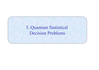
![Pathological Example
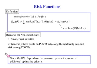
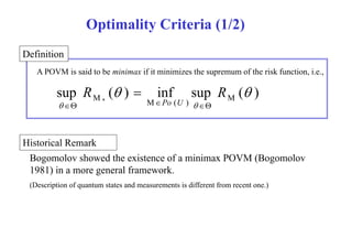
Remark
Even on a compact space, a bounded lower semicontinuous (and not
continuous) loss function does not necessarily admit a LFP.
Example [0,1]
R( )
( ) ( , ) M R L u 1
( 1
0
0 1
M M
1 sup R ( ) sup R
( ) (d )
[ 0 ,1] [ 0 ,1]
But for every prior, 1 R ( ) (d )
[ 0 ,1] M](https://image.slidesharecdn.com/slide2014rims1031public-141101055906-conversion-gate02/85/Quantum-Minimax-Theorem-in-Statistical-Decision-Theory-RIMS2014-51-320.jpg)