Downloaded 31 times


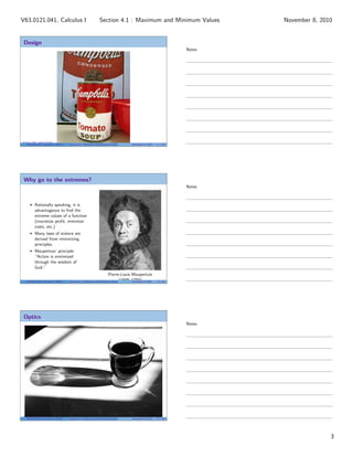
![The Extreme Value Theorem
Theorem (The Extreme Value Theorem)
Let f be a function which is continuous on the closed interval [a, b]. Then
f attains an absolute maximum value f (c) and an absolute minimum
value f (d) at numbers c and d in [a, b].
a b
c
maximum
maximum
value
f (c)
d
minimum
minimum
value
f (d)
V63.0121.041, Calculus I (NYU) Section 4.1 Maximum and Minimum Values November 8, 2010 13 / 34
No proof of EVT forthcoming
This theorem is very hard to prove without using technical facts
about continuous functions and closed intervals.
But we can show the importance of each of the hypotheses.
V63.0121.041, Calculus I (NYU) Section 4.1 Maximum and Minimum Values November 8, 2010 14 / 34
Bad Example #1
Example
Consider the function
f (x) =
x 0 ≤ x < 1
x − 2 1 ≤ x ≤ 2.
|
1
Then although values of f (x) get arbitrarily close to 1 and never bigger
than 1, 1 is not the maximum value of f on [0, 1] because it is never
achieved. This does not violate EVT because f is not continuous.
V63.0121.041, Calculus I (NYU) Section 4.1 Maximum and Minimum Values November 8, 2010 15 / 34
Notes
Notes
Notes
5
Section 4.1 : Maximum and Minimum ValuesV63.0121.041, Calculus I November 8, 2010](https://image.slidesharecdn.com/lesson18-maximumandminimumvalues041handout-101105172557-phpapp01/85/Lesson-18-Maximum-and-Minimum-Values-Section-041-handout-5-320.jpg)
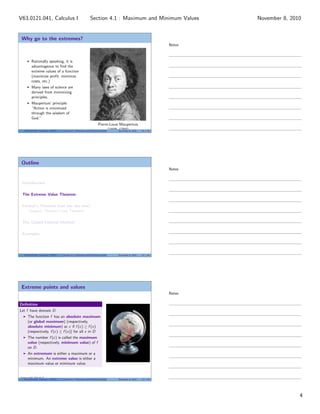
![Flowchart for placing extrema
Thanks to Fermat
Suppose f is a continuous function on the closed, bounded interval [a, b],
and c is a global maximum point.
start
Is c an
endpoint?
c = a or
c = b
c is a
local max
Is f
diff’ble at
c?
f is not
diff at c
f (c) = 0
no
yes
no
yes
V63.0121.041, Calculus I (NYU) Section 4.1 Maximum and Minimum Values November 8, 2010 26 / 34
The Closed Interval Method
This means to find the maximum value of f on [a, b], we need to:
Evaluate f at the endpoints a and b
Evaluate f at the critical points or critical numbers x where either
f (x) = 0 or f is not differentiable at x.
The points with the largest function value are the global maximum
points
The points with the smallest or most negative function value are the
global minimum points.
V63.0121.041, Calculus I (NYU) Section 4.1 Maximum and Minimum Values November 8, 2010 27 / 34
Outline
Introduction
The Extreme Value Theorem
Fermat’s Theorem (not the last one)
Tangent: Fermat’s Last Theorem
The Closed Interval Method
Examples
V63.0121.041, Calculus I (NYU) Section 4.1 Maximum and Minimum Values November 8, 2010 28 / 34
Notes
Notes
Notes
9
Section 4.1 : Maximum and Minimum ValuesV63.0121.041, Calculus I November 8, 2010](https://image.slidesharecdn.com/lesson18-maximumandminimumvalues041handout-101105172557-phpapp01/85/Lesson-18-Maximum-and-Minimum-Values-Section-041-handout-9-320.jpg)
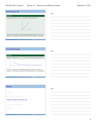
![Extreme values of a linear function
Example
Find the extreme values of f (x) = 2x − 5 on [−1, 2].
Solution
Since f (x) = 2, which is never zero, we have no critical points and we
need only investigate the endpoints:
f (−1) = 2(−1) − 5 = −7
f (2) = 2(2) − 5 = −1
So
The absolute minimum (point) is at −1; the minimum value is −7.
The absolute maximum (point) is at 2; the maximum value is −1.
V63.0121.041, Calculus I (NYU) Section 4.1 Maximum and Minimum Values November 8, 2010 29 / 34
Extreme values of a quadratic function
Example
Find the extreme values of f (x) = x2
− 1 on [−1, 2].
Solution
We have f (x) = 2x, which is zero when x = 0. So our points to check
are:
f (−1) = 0
f (0) = − 1 (absolute min)
f (2) = 3 (absolute max)
V63.0121.041, Calculus I (NYU) Section 4.1 Maximum and Minimum Values November 8, 2010 30 / 34
Extreme values of a cubic function
Example
Find the extreme values of f (x) = 2x3
− 3x2
+ 1 on [−1, 2].
Solution
V63.0121.041, Calculus I (NYU) Section 4.1 Maximum and Minimum Values November 8, 2010 31 / 34
Notes
Notes
Notes
10
Section 4.1 : Maximum and Minimum ValuesV63.0121.041, Calculus I November 8, 2010](https://image.slidesharecdn.com/lesson18-maximumandminimumvalues041handout-101105172557-phpapp01/85/Lesson-18-Maximum-and-Minimum-Values-Section-041-handout-10-320.jpg)
![Extreme values of an algebraic function
Example
Find the extreme values of f (x) = x2/3
(x + 2) on [−1, 2].
Solution
V63.0121.041, Calculus I (NYU) Section 4.1 Maximum and Minimum Values November 8, 2010 32 / 34
Extreme values of another algebraic function
Example
Find the extreme values of f (x) = 4 − x2 on [−2, 1].
Solution
V63.0121.041, Calculus I (NYU) Section 4.1 Maximum and Minimum Values November 8, 2010 33 / 34
Summary
The Extreme Value Theorem: a continuous function on a closed
interval must achieve its max and min
Fermat’s Theorem: local extrema are critical points
The Closed Interval Method: an algorithm for finding global extrema
V63.0121.041, Calculus I (NYU) Section 4.1 Maximum and Minimum Values November 8, 2010 34 / 34
Notes
Notes
Notes
11
Section 4.1 : Maximum and Minimum ValuesV63.0121.041, Calculus I November 8, 2010](https://image.slidesharecdn.com/lesson18-maximumandminimumvalues041handout-101105172557-phpapp01/85/Lesson-18-Maximum-and-Minimum-Values-Section-041-handout-11-320.jpg)

The document discusses the concepts of maximum and minimum values in calculus, focusing on the Extreme Value Theorem and Fermat's Theorem. It outlines methods for finding extreme values via the closed interval method, emphasizing the importance of continuity and differentiability. Examples illustrate these concepts in practice, confirming the role of critical points and endpoints in determining global extrema.


![5G Explained! A High Level Overview [Introduction]](https://cdn.slidesharecdn.com/ss_thumbnails/5gexplainedahighleveloverview-260119165306-cc137a3e-thumbnail.jpg?width=640&height=640&fit=bounds)


