This document provides instructions for using Microsoft Excel 2010. It covers how to open Excel, enter and format data, use formulas and functions to calculate totals, insert a column chart, apply themes and styles, and add a header and footer. The instructions culminate in saving the Excel worksheet as a file in the specified folder on the H: drive.

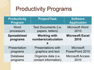
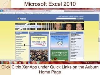
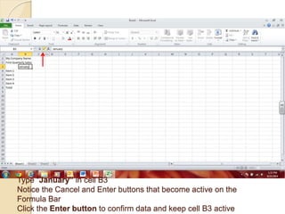
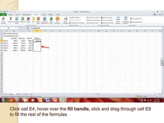
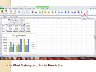
1. Productivity Programs
Microsoft Excel 2010
Tech Lit

2. Productivity Programs
Productivity
Program
Project/Task Software
Application
Word
processors
Text Documents (i.e.
papers, letters)
Microsoft Word
2010
Spreadsheet
programs
Working with
numbers/calculation
s
Microsoft Excel
2010
Presentation
programs
Presentations with
graphics and text
Microsoft
PowerPoint 2010
Database
programs
Organize data (i.e.
contact information)
Microsoft Access
2010

3. Microsoft Excel
Store, organize, use and modify data
Perform calculations
Create charts and graphs

4. Microsoft Excel 2010
Opening from
Computer
Desktop
Click the Start Button, Click All Programs

5. Microsoft Excel 2010
Opening from
Computer
Desktop
Click Microsoft Office Folder to open, click Microsoft
Office Excel 2010 to open

6. Microsoft Excel 2010
A blank Excel spreadsheet will open

7. Microsoft Excel 2010
Opening from
Double Click Internet Explorer Shortcut on the
desktop
Citrix

8. Microsoft Excel 2010
Click Citrix XenApp under Quick Links on the Auburn
Home Page

9. Microsoft Excel 2010
Enter User Name and Password, Click Log On

10. Microsoft Excel 2010
Double Click Office 2010 Folder to open

11. Microsoft Excel 2010
Double Click Excel 2010 to open

12. Microsoft Excel 2010
Auburn Acceptable Use Notice, Click OK

13. Microsoft Excel 2010
If this message appears, choose “Use
Recommended Settings” and click OK

14. Microsoft Excel 2010
A blank Excel spreadsheet will open

15. Microsoft Excel 2007
The Excel Window
http://www.swotster.com/swotster/English/Excel2010/images/images_les_001/les01_image002_en.jpg

16. Enter Company Name in cell A1
Click Enter to confirm data you entered

17. Enter First Quarterly Sales in cell A2
Click Enter

18. Click Enter again to make A4 active
Type an item name in A4 and click Enter

19. Type another item name in A5
Notice AutoComplete feature

20. Type in additional inventory items in cells A6
and A7
Type “Total” in cell A8; click Enter

21. Type “January” in cell B3
Notice the Cancel and Enter buttons that become active on the
Formula Bar
Click the Enter button to confirm data and keep cell B3 active

22. Hover over the small black square in the lower right corner of cell B3
Black crosshairs will appear – the fill handle

23. Click on the fill handle and drag to cell D3
Click the drop down arrow on the Auto Fill Options button to see
options, Fill Series should be marked

24. Click CTRL + HOME to make cell A1 active

25. Notice that the text in cell A1 is longer than column A
Point to the vertical line between columns A and B

26. Double click on the vertical line between columns A and B to Autofit or
manually drag the pointer to adjust column A’s width

27. Click Undo to undo changing the width of column A

28. Click cell B3 and drag to highlight/select cells B3:D3
Click the Center button to center the months text

29. Click cell B4 and enter a sales amount (564.23)
Press TAB to confirm data and move active cell to the right

30. Continue entering the rest of your sales numbers as shown above
Use ENTER, TAB or ARROW keys to move cells

31. Click in cell B8 and type =b4+b5+b6+b7

32. Click Enter
Notice the Total

33. Click in Cell C8, click the Formulas Tab, click AutoSum, click Sum

34. Notice the SUM Formula and the range
Click ENTER

35. Notice the Total

36. Click in cell D8, type =SUM(
Select cells D4, D5, D6 and D7
Type ) to close the formula; Click ENTER

37. Notice the TOTAL

38. Click in Cell E3, type TOTAL, click Enter

39. Click ALT = to enter the SUM function in cell E4
Click ENTER

40. Notice the Total

41. Click cell E4, hover over the fill handle, click and drag through cell E8
to fill the rest of the formulas

42. Notice Sums and AutoFill Options

43. Select cells A1:E1
Click Home Tab, click Merge and Center in Alignment Group

44. Notice how cells A1:E1 are merged into one cell and the text is
centered in that cell

45. With cells A1:E1 still selected, click Cell Styles, Click Title style

46. Select cells A2:E2, click Merge & Center

47. With cells A2:E2 still selected, click Cell Styles, click Heading 1

48. Select cells B3:E3, hold down CTRL and select cells A4:A8

49. Click Cell Styles, click Heading 4 to apply this style to cells B3:E3 and
cells A4:A8

50. Select cells B4:E4, click CTRL and select cells B8:E8

51. On the Home Tab, in the Number Group, click the Accounting
Number Format button $
Notice the numbers in cells B4:E4 and B8:E8

52. Select cells B5:E7, click the Comma Style in the Number Group

53. Select cells B8:E8, click Cell Styles, click Total style

54. Click the Page Layout tab, click Themes, click a theme (your choice)
to apply

55. Notice the Theme (font, colors, etc.) changes

56. Select cells A3:D7

57. With cells A3:D7 selected, click Insert Tab, click Columns in Charts
Group, click Clustered Column (first 2D option) chart to insert

58. Point to the top of the chart, click and drag chart to line up with cell A10

59. On the Design Tab, in the Data Group, click Switch Rows/Columns

60. Notice the category labels changed

61. On the Design tab, in the Chart Layouts group, click the More button

62. Click Layout 1, notice chart changes

63. Click to select the Chart Title, type 1st Quarter Sales, click off Chart
Title to deselect

64. In the Chart Styles group, click the More button

65. Click a style (your choice) to apply, notice changes

66. Click off of the Chart to deselect it
Click the Insert Tab, in the Text group, click Header & Footer

67. In the Navigation group, click Go to Footer

68. Click in the Left Footer Pane, in the Header & Footer Elements group,
click File Name, click cell above Footer area to exit Header & Footer

69. Click the Page Layout tab, in the Page Setup group, click Margins,
click Custom Margins

70. In the Page Setup dialog Box, under Center on page, select
Horizontally, click Print Preview

71. Notice how the data and chart are centered on the page horizontally

72. Click the Home tab to close print preview

73. Click File, click Save As

74. In the left navigation pane, scroll down, click Computer

75. Scroll down to and click your student number (H: drive under Network
Location)

76. Scroll down to and double click your Tech Lit folder

77. Scroll down to and double click your Excel Assignments folder

78. Name the excel worksheet, YourName_Excel_1, click Save

79. Notice the file name changed, click X to close Excel