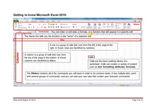
This document provides instructions for using basic spreadsheet functions in Microsoft Excel, including: - Creating a new blank spreadsheet and opening existing spreadsheets - Understanding the basic components of a spreadsheet like rows, columns, and cells - Formatting numbers and applying number formats like currency, percentages, and dates - Using functions like Sum to automatically calculate totals - Creating basic charts like column and pie charts and customizing them with titles, labels, and legends

1. Qdos Training Ltd © 2014 Dharmesh Rajput Page 1 of 12
City & Guilds
Start IT Entry 3
Unit 010 Spreadsheets

2. Qdos Training Ltd © 2014 Dharmesh Rajput Page 2 of 12
Unit 010 Spreadsheets
A spreadsheet is an interactive computer application program for organization,
analysis and storage of data in tabular form. Spreadsheets developed as
computerized simulations of paper accounting worksheets. The program operates on
data represented as cells of an array, organized in rows and columns.
Microsoft Excel is a spreadsheet program that allows you to store, organize, and
analyse information.
How to create a blank Microsoft Excel
Click on Excel icon on the taskbar.
It will open Microsoft Excel window as below:

3. Dharmesh Rajput © 2014 Page 3 of 12
Getting to know Microsoft Excel 2010:
Column
Row
Cell
Formula bar
Name box
Ribbon
A column is a group of cells that runs from
the top of the page to the bottom. In Excel,
columns are identified by letters.
A row is a group of cells that runs from the left of the page to the
right. In Excel, rows are identified by numbers.
The Name box tells you the location or the "name" of a selected cell.
You can enter or edit data, a formula, or a function that will appear in a specific cell.
The Ribbon contains all of the commands you will need in order to do common tasks. It has multiple tabs, each
with several groups of commands, and you can add your own tabs that contain your favourite commands.
Cells are the basic building blocks of a
worksheet. Cells can contain a variety of content
such as text, formatting attributes, formulas,
and functions.

4. Dharmesh Rajput © 2014 Page 4 of 12
To open an existing workbook:
1. Click the File tab.
2. Select Open. The Open dialog box appears as below:
3. Select your desired workbook, and then click Open.
Change the layout to Landscape
1. Click on Page Layout tab
2. Click on Orientation.
3. Click on Landscape.

5. Dharmesh Rajput © 2014 Page 5 of 12
Formatting the Numbers
Excel 2010 provides a variety of number formats that you can apply to the values
(numbers) you enter in a worksheet to make the data easier to interpret. These
number formats include currency, accounting, percentage, date, time, fraction, and
scientific, as well as a few special formats.
Here are some examples:
Currency: If you enter a financial value complete with the dollar sign and two
decimal places, Excel assigns a Currency number format to the cell along with the
entry.
Percentages: If you enter a value representing a percentage as a whole number
followed by the percent sign without any decimal places, Excel assigns to the cell the
Percentage number format.
Dates: If you enter a date (dates are values, too) that follows one of the built-in Excel
number formats, such as 11/10/09 or 10-Nov-09, the program assigns a Date
number format that follows the pattern of the date.
How to apply formatting to numbers
1. Select the cell/cells you want to
modify. (e.g. B2:C19)
2. Click the drop-down arrow next to
the Number Format command on
the Home tab.
3. Select the number format you
want. (e.g. we are selecting
Currency.)
You will see the new formatted numbers like this:

6. Dharmesh Rajput © 2014 Page 6 of 12
Use a Sum() Function
1. Click in the cell where you want to apply the Sum() function. (E.g. B14)
2. Click on the Home tab.
3. In the Editing group, click on the AutoSum drop-down arrow and
select Sum function
4. A formula will appear in cell B14 such as below:
5. Press Enter and result will appear in the cell B14 as below:
Tip: A function is a predefined formula that
performs calculations using specific values
in a particular order. One of the key
benefits of functions is that they can save
you time since you do not have to write the
formula yourself.

7. Dharmesh Rajput © 2014 Page 7 of 12
Create a Column chart with title and axis labels
1. Highlight the data (e.g. A4:B13)
2. Click on Insert. Click on Column and click on Clustered Column chart from 2-D
column section.
3. The chart will appear on screen as object.
To enter Title of the chart
1. Click on Layout tab.
2. Click on Chart Title
and
3. Above Chart to insert
a title.
4. Type the title
Outgoings and press
Enter.

8. Dharmesh Rajput © 2014 Page 8 of 12
To add X (Horizontal) and Y (Vertical) axis labels
1. Click on Axis Titles
2. Click on Primary Horizontal Axis Title
3. Select Title Below Axis.
4. Type Expenses and press Enter.
5. Click on Axis Titles
6. Click on Primary Vertical Axis Title
7. Select Rotated Title.
8. Type Costs and press Enter.

9. Dharmesh Rajput © 2014 Page 9 of 12
You have axis labels on your chart now.
Remove Legend
Click on Legend and Press Delete button on the keyboard.
Your chart will be look like this.

10. Dharmesh Rajput © 2014 Page 10 of 12
Move chart on a new sheet
1. Click on Design and select Move Chart.
2. Select New Sheet and click on OK.
The chart will appear on new sheet.
Create a Pie chart
1. Select data B1:C1 and B18:C18.
2. Click on Insert and Pie. Select 2-D Pie chart.

11. Dharmesh Rajput © 2014 Page 11 of 12
The Chart will be created as below:
To enter Title of the chart
1. Click on Layout tab.
2. Click on Chart Title.
3. Select Above Chart to insert a title.
4. Type Income and Outgoings and press Enter.
To add data labels showing percentages
1. Click on Layout tab, Data Labels and select More Data Label Options.

12. Dharmesh Rajput © 2014 Page 12 of 12
2. Select Percentages and deselect
Values.
3. Click on Close.
The Chart will be created as below: