Excel Basic-Part 1

1. MASTER IN MS-EXCEL
365

2. Master in MS- Excel 365
1. Basic Excel
Functionalities
2. Key
Functions
3. Data
Structures
4. Data
Transformation

3. Basic Excel Functionalities

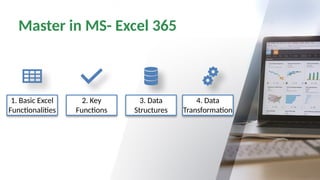
4. Step 1: Understanding the Basics
•Excel Interface: Learn about the Ribbon, Quick Access Toolbar, Formula Bar,
and Worksheets.
•Navigation: Moving between cells, rows, and columns.
•Basic Formatting: Font styles, colors, cell alignment, and borders.
•Saving & Sharing: Saving files in OneDrive, sharing with collaborators, and
exporting.

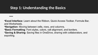
5. 1. Excel Interface
Quick Access Tool Bar
Ribbon Tab
Name Box Formula Bar/Function Bar
Group
Column
Row
Sheet
Active Cell
Title Bar
Status Bar
Scroll Bar
Working Area

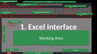
6. A. Ribbon
Located at the top, the Ribbon contains multiple
tabs (Home, Insert, Formulas, Data, etc.).
Each tab has Groups with relevant commands
(e.g., Font, Alignment, Number in the Home tab).
The File tab lets you open, save, print, and share
files.

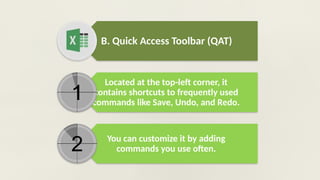
7. B. Quick Access Toolbar (QAT)
Located at the top-left corner, it
contains shortcuts to frequently used
commands like Save, Undo, and Redo.
You can customize it by adding
commands you use often.

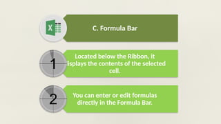
8. C. Formula Bar
Located below the Ribbon, it
displays the contents of the selected
cell.
You can enter or edit formulas
directly in the Formula Bar.

9. D. Worksheet Area
The main area where you enter data.
It consists of cells organized into columns
(A, B, C, …) and rows (1, 2, 3, …).
A cell is identified by its Cell Reference
(e.g., A1, B2, C3).

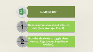
10. E. Status Bar
Displays information about selected
data (Sum, Average, Count).
Provides shortcuts to toggle views
(Normal, Page Layout, Page Break
Preview).

11. 2. Navigating in
Excel-365

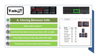
12. A. Moving Between Cells
Click a cell to select it.
Use the Arrow Keys to move up, down, left, or right.
Press Tab to move to the next cell on the right.
Press Enter to move to the next row below.

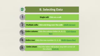
13. B. Selecting Data
Single cell: Click on a cell.
Multiple cells: Click and drag over the cells. (Shift+Arrow)
Entire column: Click the column letter (A, B, C). (Ctrl+Space
Bar)
Entire row: Click the row number (1, 2, 3).(Shift+Space Bar)
Entire sheet: Click the Select All button (top-left corner of
the sheet).(Ctrl+A)

14. C. Shortcuts
for
Navigation

15. a. Basic
Operation
Key Action Key Action Key Action
Ctrl+A Select All Ctrl+P Print Ctrl+9 Hide a
Row
Ctrl+B Bold Ctrl+R Fill Right from
Left
Ctrl+F1 Show/Hide
Ribbon
Ctrl+C Copy Cell Ctrl+S/
F12
Save Ctrl+F2 Print Preview
Ctrl+D Fill Down Ctrl+U Underline Ctrl+F3 Name a cell
Or Cell Range
Ctrl+F Find Ctrl+V Paste Ctrl+F4 Close the
Window
Ctrl+H Replace Ctrl+W Close
Workbook
Ctrl+
Spacebar
Select Entire
Column
Ctrl+I Italic Ctrl+Y Redo Ctrl+Shift
+F
Font Menu
Dialogue Box
Ctrl+K Hyperlink Ctrl+Z Undo Ctrl+Page
UP
Previous
Worksheet
Ctrl+N New Sheet Ctrl+1 Formatting
Dialogue box
Ctrl+Page
Down
Next
Worksheet
Ctrl+O Open Existing
Sheet
Ctrl+5 Strikethrough
In the cell
F2 Edit Cell

16. b. Auditing
Formula
Key Action
Ctrl+ ~ Formula View
Ctrl+[ Direct Precedents
Ctrl+] Direct Dependents
Alt  M  P Indirect Precedents
Alt  M  D Indirect Dependents
Alt  M  A  A Remove Tracing
Arrows

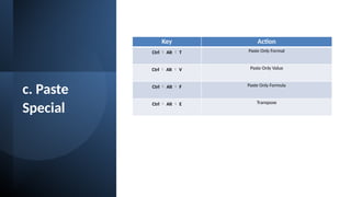
17. c. Paste
Special
Key Action
Ctrl  Alt  T Paste Only Format
Ctrl  Alt  V Paste Only Value
Ctrl  Alt  F Paste Only Formula
Ctrl  Alt  E Transpose

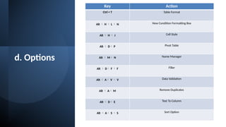
18. d. Options
Key Action
Ctrl + T Table Format
Alt  H  L  N New Condition Formatting Box
Alt  H  J Cell Style
Alt  D P Pivot Table
Alt  M N Name Manager
Alt  D F  F Filler
Alt  A V  V Data Validation
Alt  A M Remove Duplicates
Alt  D E Text To Column
Alt  A S  S Sort Option

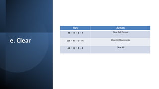
19. e. Clear
Key Action
Alt  H  E  F Clear Cell Format
Alt  H  E  M Clear Cell Comments
Alt  H  E  A Clear All

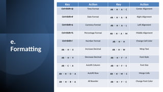
20. e.
Formatting
Key Action Key Action
Ctrl+Shift+@ Time Format Alt  H  A  C Center Alignment
Ctrl+Shift+# Date Format Alt  H  A  R Right Alignment
Ctrl+Shift+$ Currency Format Alt  H  A  L Left Alignment
Ctrl+Shift+% Percentage Format Alt  H  A  M Middle Alignment
Ctrl+Shift+! Number Format Alt  H  H Change Cell Color
Alt  H  0 Increase Decimal Alt  H  W Wrap Text
Alt  H  9 Decrease Decimal Alt  H  F  F Font Style
Alt  C  A Autofit Column Alt  H  F  S Font Size
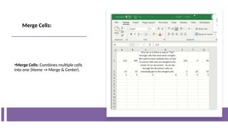
Alt  H  O  A Autofit Row Alt  H  M  C Merge Cells
Alt  H  B  A All Boarder Alt  H  F  C Change Font Color

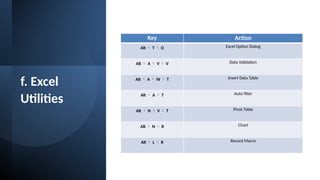
21. f. Excel
Utilities
Key Action
Alt  T  O Excel Option Dialog
Alt  A  V  V Data Validation
Alt  A  W  T Insert Data Table
Alt  A  T Auto filter
Alt  N  V  T Pivot Table
Alt  N  R Chart
Alt  L  R Record Macro

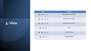
22. g. View
Key Action
Alt  W  V  F Hide/Unhide Formula Bar
Alt  W  V  H Hide/Unhide Heading
Alt  W  V  G Hide/Unhide Grid Line
Alt  W  Q Zoom
Alt  W  Q  C Customize Zoom
Alt  W  A Arrange Window

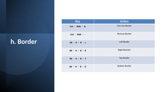
23. h. Border
Key Action
Ctrl  Shift  & Out Line Border
Ctrl  Shift  - Remove Border
Alt  H  B  L Left Border
Alt  H  B  R Right Boarder
Alt  H  B  T Top Border
Alt  H  B  O Bottom Border

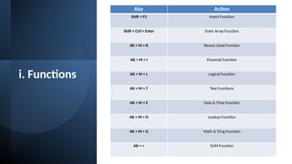
24. i. Functions
Key Action
Shift + F3 Insert Function
Shift + Ctrl + Enter Enter Array Function
Alt + M + R Recent Used Function
Alt + M + I Financial Function
Alt + M + L Logical Function
Alt + M + T Text Functions
Alt + M + E Date & Time Function
Alt + M + O Lookup Function
Alt + M + G Math & Tring Function
Alt + = SUM Function

25. j.
Navigation
Key Action
Alt  H  O  R Rename Worksheet
Alt  H  O  M Rearrange Sheet Tab Order
F1 Help Box

26. k. Row &
Column
Key Action
Ctrl + - Delete Row/Column
Ctrl + Shift + + Add Row/Column
Alt + Shift + Right Group Row/Column
Alt + Shift + Left Ungroup Row/Column

27. •3. Basic Formatting in
Excel

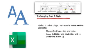
28. •Select a cell or range, then use the Home → Font
group to:
• Change font type, size, and color.
• Apply Bold (Ctrl + B), Italic (Ctrl + I), or
Underline (Ctrl + U).
A. Changing Font & Style

29. Use the Alignment
group to:
Align text Left,
Center, or Right.
Adjust Vertical
Alignment (Top,
Middle, Bottom).
Wrap Text: Keeps all
text visible in a cell
without
overflowing.
B. Aligning Text

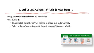
30. •Drag the column/row border to adjust size.
•Use AutoFit:
• Double-click the column/row border to adjust size automatically.
• Select column/row → Home → Format → AutoFit Column Width.
C. Adjusting Column Width & Row Height

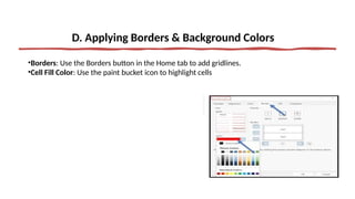
31. •Borders: Use the Borders button in the Home tab to add gridlines.
•Cell Fill Color: Use the paint bucket icon to highlight cells
D. Applying Borders & Background Colors

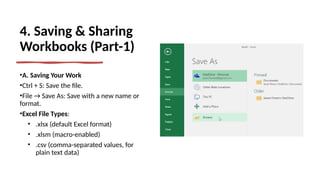
32. 4. Saving & Sharing
Workbooks (Part-1)
•A. Saving Your Work
•Ctrl + S: Save the file.
•File → Save As: Save with a new name or
format.
•Excel File Types:
• .xlsx (default Excel format)
• .xlsm (macro-enabled)
• .csv (comma-separated values, for
plain text data)

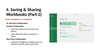
33. 4. Saving & Sharing
Workbooks (Part-2)
•B. Sharing & Collaboration
•OneDrive Integration:
• Save files online to access from any
device.
• Share files with others using File →
Share.
•Real-Time Collaboration:
• If stored in OneDrive, multiple users can
edit the same file at the same time.

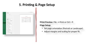
34. •Print Preview: File → Print or Ctrl + P.
•Page Setup:
• Set page orientation (Portrait or Landscape).
• Adjust margins and scaling for proper fit.
5. Printing & Page Setup

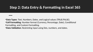
35. Step 2: Data Entry & Formatting in Excel 365
•Data Types: Text, Numbers, Dates, and Logical values (TRUE/FALSE).
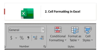
•Cell Formatting: Number format (Currency, Percentage, Date), Conditional
Formatting, and Custom Formatting.
•Data Validation: Restricting input using lists, numbers, and dates.

36. 1. Data Types
in Excel

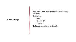
37. •Any letters, words, or combinations of numbers
and letters.
•Examples:
• "Hello"
• "Excel 365"
• "123ABC"
•Behavior: Left-aligned by default.
A. Text (String)

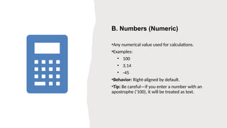
38. •Any numerical value used for calculations.
•Examples:
• 100
• 3.14
• -45
•Behavior: Right-aligned by default.
•Tip: Be careful—if you enter a number with an
apostrophe ('100), it will be treated as text.
B. Numbers (Numeric)

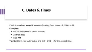
39. •Excel stores dates as serial numbers (starting from January 1, 1900, as 1).
•Examples:
• 03/23/2025 (MM/DD/YYYY format)
• 23-Mar-2025
• 8:30 AM
•Tip: Use Ctrl + ; for today’s date and Ctrl + Shift + ; for the current time.
C. Dates & Times

40. •Represented by TRUE or FALSE.
•Used in formulas and conditions.
•Example:
• =A1>50 → Returns TRUE if the value
in A1 is greater than 50.
•Behavior: Excel treats TRUE as 1 and
FALSE as 0 in calculations.
D. Logical Values (Boolean)

41. 2. Cell Formatting in Excel

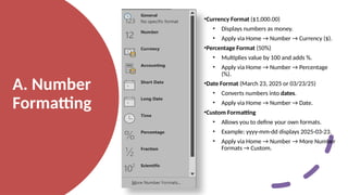
42. •Currency Format ($1,000.00)
• Displays numbers as money.
• Apply via Home → Number → Currency ($).
•Percentage Format (50%)
• Multiplies value by 100 and adds %.
• Apply via Home → Number → Percentage
(%).
•Date Format (March 23, 2025 or 03/23/25)
• Converts numbers into dates.
• Apply via Home → Number → Date.
•Custom Formatting
• Allows you to define your own formats.
• Example: yyyy-mm-dd displays 2025-03-23.
• Apply via Home → Number → More Number
Formats → Custom.
A. Number
Formatting

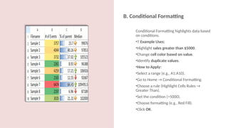
43. Conditional Formatting highlights data based
on conditions.
•📌 Example Uses:
•Highlight sales greater than $5000.
•Change cell color based on value.
•Identify duplicate values.
•How to Apply:
•Select a range (e.g., A1:A10).
•Go to Home → Conditional Formatting.
•Choose a rule (Highlight Cells Rules →
Greater Than).
•Set the condition (>5000).
•Choose formatting (e.g., Red Fill).
•Click OK.
B. Conditional Formatting

44. C. Wrap Text &
Merge Cells

45. •Wrap Text: Displays long text in a single cell without
spilling over. (Home → Wrap Text).

46. •Merge Cells: Combines multiple cells
into one (Home → Merge & Center).
Merge Cells:

47. 3. Data
Validation

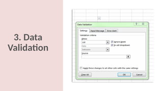
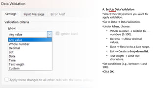
48. A. Set Up Data Validation
•Select the cell(s) where you want to
apply validation.
•Go to Data → Data Validation.
•Under Allow, choose:
• Whole number → Restrict to
numbers (1-100).
• Decimal → Allow decimal
values.
• Date → Restrict to a date range.
• List → Create a drop-down list.
• Text length → Limit text
characters.
•Set conditions (e.g., between 1 and
100).
•Click OK.

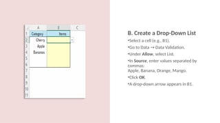
49. B. Create a Drop-Down List
•Select a cell (e.g., B1).
•Go to Data → Data Validation.
•Under Allow, select List.
•In Source, enter values separated by
commas:
Apple, Banana, Orange, Mango.
•Click OK.
•A drop-down arrow appears in B1.

50. C. Custom Error Messages
•To display an error message:
•In Data Validation, go to Error Alert.
•Set a Title (e.g., "Invalid Entry").
•Enter a Message (e.g., "Enter a
number between 1 and 100").
•Click OK.

51. Step 3: Basic Formulas & Functions
•Mathematical Functions: SUM, AVERAGE, MIN, MAX.
•Text Functions: LEFT, RIGHT, MID, LEN, TRIM, CONCATENATE, TEXTJOIN).
•Logical Functions: IF, AND, OR, IFERROR, IFS.
•Date & Time Functions: TODAY(), NOW(), DATEDIF, TEXT.

52. 1. Understanding Formulas in Excel

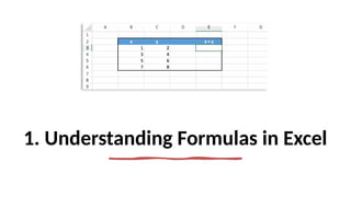
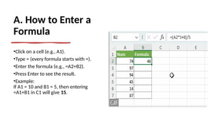
53. A. How to Enter a
Formula
•Click on a cell (e.g., A1).
•Type = (every formula starts with =).
•Enter the formula (e.g., =A2+B2).
•Press Enter to see the result.
•Example:
If A1 = 10 and B1 = 5, then entering
=A1+B1 in C1 will give 15.

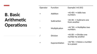
54. B. Basic
Arithmetic
Operations
Operator Function Example (=A1 B1)
+ Addition
=A1+B1 → Adds two
numbers
- Subtraction
=A1-B1 → Subtracts one
from another
* Multiplication =A1*B1 → Multiplies two
numbers
/ Division
=A1/B1 → Divides one
number by another
^ Exponentiation
=A1^B1 → Raises a number
to a power

55. 2. Commonly Used Functions
in Excel

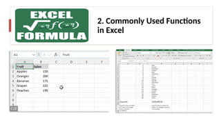
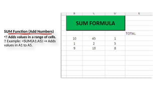
56. SUM Function (Add Numbers)
•📌 Adds values in a range of cells.
✅ Example: =SUM(A1:A5) → Adds
values in A1 to A5.

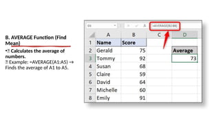
57. B. AVERAGE Function (Find
Mean)
•📌 Calculates the average of
numbers.
✅ Example: =AVERAGE(A1:A5) →
Finds the average of A1 to A5.

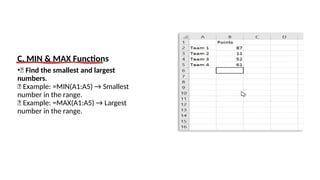
58. C. MIN & MAX Functions
•📌 Find the smallest and largest
numbers.
✅ Example: =MIN(A1:A5) → Smallest
number in the range.
✅ Example: =MAX(A1:A5) → Largest
number in the range.

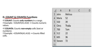
59. D. COUNT & COUNTA Functions
•📌 COUNT: Counts only numbers in a range.
✅ Example: =COUNT(A1:A10) → Counts numeric
values.
•📌 COUNTA: Counts non-empty cells (text or
numbers).
✅ Example: =COUNTA(A1:A10) → Counts filled
cells.

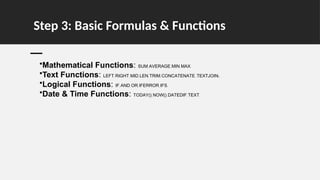
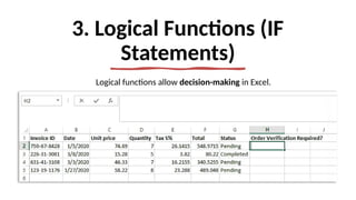
60. 3. Logical Functions (IF
Statements)
Logical functions allow decision-making in Excel.

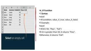
61. •A. IF Function
•📌 Syntax:
•excel
•=IF(condition, value_if_true, value_if_false)
•✅ Example:
•excel
•=IF(A1>50, "Pass", "Fail")
•If A1 is greater than 50, it returns "Pass".
•Otherwise, it returns "Fail".

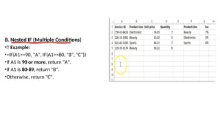
62. B. Nested IF (Multiple Conditions)
•📌 Example:
•=IF(A1>=90, "A", IF(A1>=80, "B", "C"))
•If A1 is 90 or more, return "A".
•If A1 is 80-89, return "B".
•Otherwise, return "C".

63. 4. Combining Functions
You can combine multiple functions for advanced calculations.

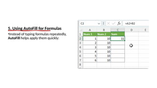
64. 5. Using AutoFill for Formulas
•Instead of typing formulas repeatedly,
AutoFill helps apply them quickly:

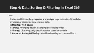
65. Step 4: Data Sorting & Filtering in Excel 365
Sorting and filtering help organize and analyze large datasets efficiently by
arranging or displaying only relevant data.
In this step, we’ll cover:
✅ Sorting: Arranging data in ascending/descending order.
✅ Filtering: Displaying only specific records based on criteria.
✅ Advanced Sorting & Filtering: Multi-level sorting and custom filters.

66. 1. Sorting Data in Excel
Sorting helps you arrange data alphabetically,
numerically, or by date.

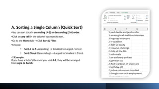
67. A. Sorting a Single Column (Quick Sort)
•You can sort data in ascending (A-Z) or descending (Z-A) order.
•Click on any cell in the column you want to sort.
•Go to the Home tab → Click Sort & Filter.
•Choose:
• Sort A to Z (Ascending) → Smallest to Largest / A to Z.
• Sort Z to A (Descending) → Largest to Smallest / Z to A.
•📌 Example:
If you have a list of cities and you sort A-Z, they will be arranged
from Agra to Zurich.

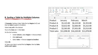
68. B. Sorting a Table by Multiple Columns
•📌 Example: Sorting a Sales Table first by Region (A-Z) and
then by Sales (Largest to Smallest).
•Select any cell in the dataset.
•Go to the Data tab → Click Sort.
•In the Sort window:
• Under Column, select Region → Choose A to Z.
• Click Add Level.
• Select Sales → Choose Largest to Smallest.
•Click OK.
•✔ Now, your data is sorted first by Region, then by Sales
within each region.

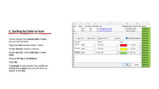
69. C. Sorting by Color or Icon
•If your dataset has colored cells or icons,
you can sort by those.
•Open the Sort window (Data → Sort).
•Under Sort by, choose a column.
•Under Sort On, select Cell Color or Font
Color.
•Choose On Top or On Bottom.
•Click OK.
•📌 Example: If sales greater than $5000 are
highlighted in green, you can sort them to
appear at the top.

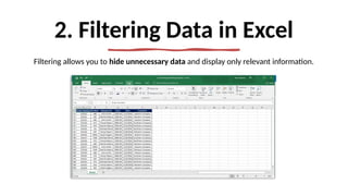
70. 2. Filtering Data in Excel
Filtering allows you to hide unnecessary data and display only relevant information.

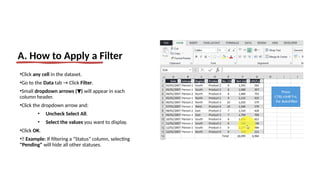
71. •Click any cell in the dataset.
•Go to the Data tab → Click Filter.
•Small dropdown arrows ( )
▼ will appear in each
column header.
•Click the dropdown arrow and:
• Uncheck Select All.
• Select the values you want to display.
•Click OK.
•📌 Example: If filtering a “Status” column, selecting
"Pending" will hide all other statuses.
A. How to Apply a Filter

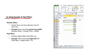
72. B. Using Number & Text Filters
•Number Filters:
• Greater than, Less than, Between, Top 10
items, etc.
• Example: Show only Sales greater than $5000
(Number Filters → Greater Than → 5000).
•Text Filters:
• Contains, Begins With, Ends With, etc.
• Example: Filter names that begin with "A"
(Text Filters → Begins With → A).

73. C. Clearing Filters
•To remove filters:
•Go to the Data tab → Click Clear.
•OR Click the filter icon ( )
▼ and select
Clear Filter from [Column].

74. 3. Advanced
Filtering
For complex
datasets, you can
use Advanced Filter
to apply custom
criteria.

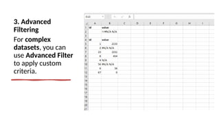
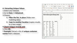
75. A. Extracting Unique Values
1.Select your dataset.
2.Go to Data → Advanced.
3.Choose:
1. Filter the list, in place (hides non-
matching data).
2. Copy to another location (copies results
to a new range).
4.Check Unique records only.
5.Click OK.
📌 Example: Extract a list of unique customer
names from a dataset.

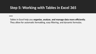
76. Step 5: Working with Tables in Excel 365
Tables in Excel help you organize, analyze, and manage data more efficiently.
They allow for automatic formatting, easy filtering, and dynamic formulas.

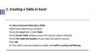
77. •A. How to Convert Data into a Table
•Select your dataset (e.g., A1:D10).
•Go to the Insert tab → Click Table.
•In the Create Table window, ensure the correct range is selected.
•Check My table has headers (if your data has column names).
•Click OK.
•✔ Your data is now formatted as a table with built-in sorting and filtering.
1. Creating a Table in Excel

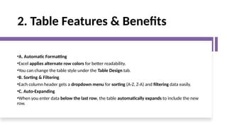
78. 2. Table Features & Benefits
•A. Automatic Formatting
•Excel applies alternate row colors for better readability.
•You can change the table style under the Table Design tab.
•B. Sorting & Filtering
•Each column header gets a dropdown menu for sorting (A-Z, Z-A) and filtering data easily.
•C. Auto-Expanding
•When you enter data below the last row, the table automatically expands to include the new
row.

79. A. Example of Structured Reference
•If your table is named SalesTable, and you want to calculate the total revenue in a new column:
•=[Price]*[Quantity]
•This formula automatically applies to the entire column.
B. Benefits of Structured References
✔ Easier to read and understand.
Automatically updates when new rows are added.
✔
Works well with functions like SUM(), AVERAGE(), etc.
✔
3. Using Structured References in Table Formulas
In Excel tables, formulas use structured references instead of cell addresses.

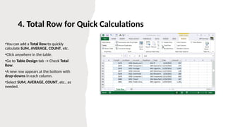
80. •You can add a Total Row to quickly
calculate SUM, AVERAGE, COUNT, etc.
•Click anywhere in the table.
•Go to Table Design tab → Check Total
Row.
•A new row appears at the bottom with
drop-downs in each column.
•Select SUM, AVERAGE, COUNT, etc., as
needed.
4. Total Row for Quick Calculations

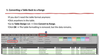
81. •If you don’t need the table format anymore:
•Click anywhere in the table.
•Go to Table Design tab → Click Convert to Range.
•Click OK → The table formatting is removed, but the data remains.
5. Converting a Table Back to a Range
1
2

82. Step 6: Data Validation in Excel 365
Data Validation helps control what type of data can be entered into a cell. It
prevents errors and ensures consistency in data entry.

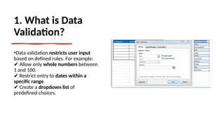
83. 1. What is Data
Validation?
•Data validation restricts user input
based on defined rules. For example:
Allow only
✔ whole numbers between
1 and 100.
Restrict entry to
✔ dates within a
specific range.
Create a
✔ dropdown list of
predefined choices.

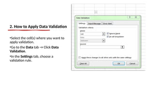
84. 2. How to Apply Data Validation
•Select the cell(s) where you want to
apply validation.
•Go to the Data tab → Click Data
Validation.
•In the Settings tab, choose a
validation rule.

85. 3. Common
Data Validation
Rules

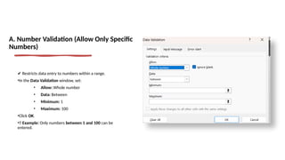
86. ✔ Restricts data entry to numbers within a range.
•In the Data Validation window, set:
• Allow: Whole number
• Data: Between
• Minimum: 1
• Maximum: 100
•Click OK.
•📌 Example: Only numbers between 1 and 100 can be
entered.
A. Number Validation (Allow Only Specific
Numbers)

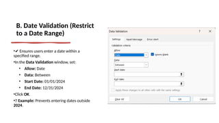
87. B. Date Validation (Restrict
to a Date Range)
•✔ Ensures users enter a date within a
specified range.
•In the Data Validation window, set:
• Allow: Date
• Data: Between
• Start Date: 01/01/2024
• End Date: 12/31/2024
•Click OK.
•📌 Example: Prevents entering dates outside
2024.

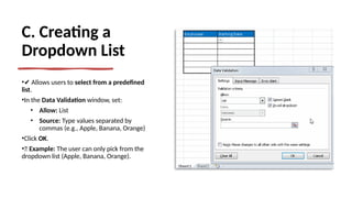
88. C. Creating a
Dropdown List
•✔ Allows users to select from a predefined
list.
•In the Data Validation window, set:
• Allow: List
• Source: Type values separated by
commas (e.g., Apple, Banana, Orange)
•Click OK.
•📌 Example: The user can only pick from the
dropdown list (Apple, Banana, Orange).

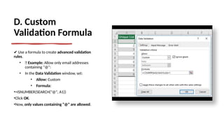
89. D. Custom
Validation Formula
✔ Use a formula to create advanced validation
rules.
• 📌 Example: Allow only email addresses
containing "@":
• In the Data Validation window, set:
• Allow: Custom
• Formula:
•=ISNUMBER(SEARCH("@", A1))
•Click OK.
•Now, only values containing “@” are allowed.

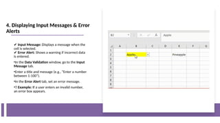
90. ✔ Input Message: Displays a message when the
cell is selected.
✔ Error Alert: Shows a warning if incorrect data
is entered.
•In the Data Validation window, go to the Input
Message tab.
•Enter a title and message (e.g., “Enter a number
between 1-100”).
•In the Error Alert tab, set an error message.
•📌 Example: If a user enters an invalid number,
an error box appears.
4. Displaying Input Messages & Error
Alerts

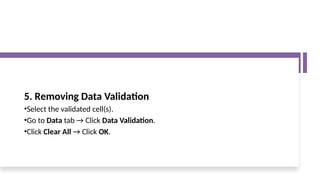
91. 5. Removing Data Validation
•Select the validated cell(s).
•Go to Data tab → Click Data Validation.
•Click Clear All → Click OK.

92. Advanced
Excel 365