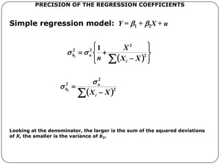
1. The document discusses the simple linear regression model and how to derive the regression coefficients using the least squares method. 2. It uses a numerical example to show how to calculate the regression coefficients b1 and b2 by minimizing the sum of squared residuals. 3. The general method is then described for a model with n observations, where the regression coefficients b1 and b2 are the values that minimize the total sum of squared residuals.

1. KTEE 309 ECONOMETRICS
THE SIMPLE REGRESSION MODEL
Chap 4 – S & W
1
Dr TU Thuy Anh
Faculty of International Economics

2. Output and labor use
2
0
50
100
150
200
250
300
1 2 3 4 5 6 7 8 9 10 11 12 13 14 15 16 17 18 19 20 21 22 23 24
Labor Output

3. 1
Output and labor use
The scatter diagram shows output q plotted against labor use l for a sample
of 24 observations
0
50
100
150
200
250
300
80 100 120 140 160 180 200 220
Output vs labor use

4. 4
Output and labor use
 Economic theory (theory of firms) predicts
An increase in labor use leads to an increase output in the
SR, as long as MPL>0, other thing being equal
 From the data:
 consistent with common sense
 the relationship looks linear
 Setting up:
 Want to know the impact of labor use on output
=>Y: output, X: labor use

5. 1
Y
SIMPLE LINEAR REGRESSION MODEL
Suppose that a variable Y is a linear function of another variable X, with
unknown parameters b1 and b2 that we wish to estimate.
XY 21 bb 
b1
XX1 X2 X3 X4

6. Suppose that we have a sample of 4 observations with X values as shown.
SIMPLE LINEAR REGRESSION MODEL
2
XY 21 bb 
b1
Y
XX1 X2 X3 X4

7. If the relationship were an exact one, the observations would lie on a
straight line and we would have no trouble obtaining accurate estimates of b1
and b2.
Q1
Q2
Q3
Q4
SIMPLE LINEAR REGRESSION MODEL
3
XY 21 bb 
b1
Y
XX1 X2 X3 X4

8. P4
In practice, most economic relationships are not exact and the actual values
of Y are different from those corresponding to the straight line.
P3
P2
P1
Q1
Q2
Q3
Q4
SIMPLE LINEAR REGRESSION MODEL
4
XY 21 bb 
b1
Y
XX1 X2 X3 X4

9. P4
To allow for such divergences, we will write the model as Y = b1 + b2X +
u, where u is a disturbance term.
P3
P2
P1
Q1
Q2
Q3
Q4
SIMPLE LINEAR REGRESSION MODEL
5
XY 21 bb 
b1
Y
XX1 X2 X3 X4

10. P4
Each value of Y thus has a nonrandom component, b1 + b2X, and a random
component, u. The first observation has been decomposed into these two
components.
P3
P2
P1
Q1
Q2
Q3
Q4
u1
SIMPLE LINEAR REGRESSION MODEL
6
XY 21 bb 
b1
Y
121 Xbb 
XX1 X2 X3 X4

11. P4
In practice we can see only the P points.
P3
P2
P1
SIMPLE LINEAR REGRESSION MODEL
7
Y
XX1 X2 X3 X4

12. P4
Obviously, we can use the P points to draw a line which is an approximation
to the line
Y = b1 + b2X. If we write this line Y = b1 + b2X, b1 is an estimate of b1 and b2
is an estimate of b2.
P3
P2
P1
^
SIMPLE LINEAR REGRESSION MODEL
8
XbbY 21
ˆ 
b1
Y
XX1 X2 X3 X4

13. P4
The line is called the fitted model and the values of Y predicted by it are
called the fitted values of Y. They are given by the heights of the R points.
P3
P2
P1
R1
R2
R3 R4
SIMPLE LINEAR REGRESSION MODEL
9
XbbY 21
ˆ 
b1
Yˆ
(fitted value)
Y (actual value)
Y
XX1 X2 X3 X4

14. P4
XX1 X2 X3 X4
The discrepancies between the actual and fitted values of Y are known as the
residuals.
P3
P2
P1
R1
R2
R3 R4
(residual)
e1
e2
e3
e4
SIMPLE LINEAR REGRESSION MODEL
10
XbbY 21
ˆ 
b1
Yˆ
(fitted value)
Y (actual value)
eYY  ˆ
Y

15. P4
Note that the values of the residuals are not the same as the values of the
disturbance term. The diagram now shows the true unknown relationship as
well as the fitted line.
The disturbance term in each observation is responsible for the divergence
between the nonrandom component of the true relationship and the actual
observation.
P3
P2
P1
SIMPLE LINEAR REGRESSION MODEL
12
Q2
Q1
Q3
Q4
XbbY 21
ˆ 
XY 21 bb 
b1
b1
Yˆ
(fitted value)
Y (actual value)
Y
XX1 X2 X3 X4
unknown PRF
estimated
SRF

16. P4
The residuals are the discrepancies between the actual and the fitted values.
If the fit is a good one, the residuals and the values of the disturbance term
will be similar, but they must be kept apart conceptually.
P3
P2
P1
R1
R2
R3 R4
SIMPLE LINEAR REGRESSION MODEL
13
XbbY 21
ˆ 
XY 21 bb 
b1
b1
Yˆ
(fitted value)
Y (actual value)
Y
XX1 X2 X3 X4
unknown PRF
estimated
SRF

17. 17
  L
bb
Min
i
XbbY
bb
Min
i
e
bb
MinRSS
bb
Min
eXbbY
eXbbY
2
,
1
2
21
2
,
1
2
2
,
12
,
1
21
21
 


You must prevent negative residuals from cancelling positive ones, and one
way to do this is to use the squares of the residuals.
We will determine the values of b1 and b2 that minimize RSS, the sum of the squares of the
residuals.
Least squares criterion:

18. 0
1
2
3
4
5
6
0 1 2 3
1Y
2Y
3Y
DERIVING LINEAR REGRESSION COEFFICIENTS
Y
XbbY
uXY
21
21
ˆ:lineFitted
:modelTrue

 bb
X
This sequence shows how the regression coefficients for a simple regression model are
derived, using the least squares criterion (OLS, for ordinary least squares)
We will start with a numerical example with just three observations: (1,3), (2,5), and (3,6)
1

19. 0
1
2
3
4
5
6
0 1 2 3
1Y
2Y
3Y
211
ˆ bbY 
212 2ˆ bbY 
213 3ˆ bbY 
DERIVING LINEAR REGRESSION COEFFICIENTS
Y
b2
b1
X
Writing the fitted regression as Y = b1 + b2X, we will determine the values of b1 and b2 that
minimize RSS, the sum of the squares of the residuals.
3
^
XbbY
uXY
21
21
ˆ:lineFitted
:modelTrue

 bb

20. 0
1
2
3
4
5
6
0 1 2 3
1Y
2Y
3Y
211
ˆ bbY 
212 2ˆ bbY 
213 3ˆ bbY 
Given our choice of b1 and b2, the residuals are as shown.
DERIVING LINEAR REGRESSION COEFFICIENTS
Y
b2
b1
21333
21222
21111
36ˆ
25ˆ
3ˆ
bbYYe
bbYYe
bbYYe



4
XbbY
uXY
21
21
ˆ:lineFitted
:modelTrue

 bb
X
2
21
2
21
2
21
2
3
2
2
2
1 )36()25()3( bbbbbbeeeRSS 

21. SIMPLE REGRESSION ANALYSIS
0281260 21
1



bb
b
RSS
06228120 21
2



bb
b
RSS
50.1,67.1 21  bb
The first-order conditions give us two equations in two unknowns. Solving them, we find
that RSS is minimized when b1 and b2 are equal to 1.67 and 1.50, respectively.
10
2
21
2
21
2
21
2
3
2
2
2
1 )36()25()3( bbbbbbeeeRSS 

22. 0
1
2
3
4
5
6
0 1 2 3
1Y
2Y
3Y
17.3ˆ1 Y
67.4ˆ2 Y
17.6ˆ3 Y
DERIVING LINEAR REGRESSION COEFFICIENTS
Y
XY
uXY
50.167.1ˆ:lineFitted
:modelTrue 21

 bb
X
The fitted line and the fitted values of Y are as shown.
12
1.50
1.67

23. DERIVING LINEAR REGRESSION COEFFICIENTS
XXnX1
Y
XbbY
uXY
21
21
ˆ:lineFitted
:modelTrue

 bb
1Y
nY
Now we will do the same thing for the general case with n observations.
13

24. DERIVING LINEAR REGRESSION COEFFICIENTS
XXnX1
Y
b1
XbbY
uXY
21
21
ˆ:lineFitted
:modelTrue

 bb
1211
ˆ XbbY 
1Y
b2
nY
nn XbbY 21
ˆ 
Given our choice of b1 and b2, we will obtain a fitted line as shown.
14

25. DERIVING LINEAR REGRESSION COEFFICIENTS
The residual for the first observation is defined.
Similarly we define the residuals for the remaining observations. That for the last one is
marked.
XXnX1
Y
b1
XbbY
uXY
21
21
ˆ:lineFitted
:modelTrue

 bb
nnnnn XbbYYYe
XbbYYYe
21
1211111
ˆ
.....
ˆ


1211
ˆ XbbY 
1Y
b2
nY
1e
ne nn XbbY 21
ˆ 
16

26. 26
  L
bb
Min
i
XbbY
bb
Min
i
e
bb
MinRSS
bb
Min
eXbbY
eXbbY
2
,
1
2
21
2
,
1
2
2
,
12
,
1
21
21
 


We will determine the values of b1 and b2 that minimize RSS, the sum of the squares of the
residuals.
Least squares criterion:

27. DERIVING LINEAR REGRESSION COEFFICIENTS
XXnX1
Y
b1
XbbY
uXY
21
21
ˆ:lineFitted
:modelTrue

 bb
1211
ˆ XbbY 
1Y
b2
nY
nn XbbY 21
ˆ 
XbYb 21 
We chose the parameters of the fitted line so as to minimize the sum of the squares of the
residuals. As a result, we derived the expressions for b1 and b2 using the first order
condition
40
  
 



 22
XX
YYXX
b
i
ii

28. Practice – calculate b1 and b2
Year Output - Y Labor - X
1899 100 100
1900 101 105
1901 112 110
1902 122 118
1903 124 123
1904 122 116
1905 143 125
1906 152 133
1907 151 138
1908 126 121
1909 155 140
1910 159 144
1911 153 145
28

29. 29
Model 1: OLS, using observations 1899-1922 (T = 24)
Dependent variable: q
coefficient std. error t-ratio p-value
---------------------------------------------------------
const -38,7267 14,5994 -2,653 0,0145 **
l 1,40367 0,0982155 14,29 1,29e-012 ***
Mean dependent var 165,9167 S.D. dependent var 43,75318
Sum squared resid 4281,287 S.E. of regression 13,95005
R-squared 0,902764 Adjusted R-squared 0,898344
F(1, 22) 204,2536 P-value(F) 1,29e-12
Log-likelihood -96,26199 Akaike criterion 196,5240
Schwarz criterion 198,8801 Hannan-Quinn 197,1490
rho 0,836471 Durbin-Watson 0,763565
INTERPRETATION OF A REGRESSION EQUATION
This is the output from a regression of output q, using gretl.

30. 30
80
100
120
140
160
180
200
220
240
260
100 120 140 160 180 200
q
l
q versus l (with least squares fit)
Y = -38,7 + 1,40X
Here is the scatter diagram again, with the regression line
shown

31. 31
THE COEFFICIENT OF DETERMINATION
 Question: how does the sample regression line fit the data at
hand?
 How much does the independent var. explain the variation in
the dependent var. (in the sample)?
 We have:
2
2
2
ˆ( )
( )
i
i
i
i
Y Y
R
Y Y





2 2 2ˆ( ) ( )i i i
i i i
Y Y Y Y e     
total variation
of Y
The share
explained
by model

32. GOODNESS OF FIT
RSSESSTSS 




 2
2
2
)(
)ˆ(
YY
YY
TSS
ESS
R
i
i
      222
ˆ iii eYYYY
The main criterion of goodness of fit, formally described as the coefficient of
determination, but usually referred to as R2, is defined to be the ratio of ESS
to TSS, that is, the proportion of the variance of Y explained by the
regression equation.

33. GOODNESS OF FIT





 2
2
2
)(
1
YY
e
TSS
RSSTSS
R
i
i




 2
2
2
)(
)ˆ(
YY
YY
TSS
ESS
R
i
i
The OLS regression coefficients are chosen in such a way as to minimize the
sum of the squares of the residuals. Thus it automatically follows that they
maximize R2.
      222
ˆ iii eYYYY RSSESSTSS 

34. 34
Model 1: OLS, using observations 1899-1922 (T = 24)
Dependent variable: q
coefficient std. error t-ratio p-value
---------------------------------------------------------
const -38,7267 14,5994 -2,653 0,0145 **
l 1,40367 0,0982155 14,29 1,29e-012 ***
Mean dependent var 165,9167 S.D. dependent var 43,75318
Sum squared resid 4281,287 S.E. of regression 13,95005
R-squared 0,902764 Adjusted R-squared 0,898344
F(1, 22) 204,2536 P-value(F) 1,29e-12
Log-likelihood -96,26199 Akaike criterion 196,5240
Schwarz criterion 198,8801 Hannan-Quinn 197,1490
rho 0,836471 Durbin-Watson 0,763565
INTERPRETATION OF A REGRESSION EQUATION
This is the output from a regression of output q, using gretl.

35. BASIC (Gauss-Makov) ASSUMPTION OF THE OLS
35
1. zero systematic error: E(ui) =0
2. Homoscedasticity: var(ui) = δ2 for all i
3. No autocorrelation: cov(ui; uj) = 0 for all i #j
4. X is non-stochastic
5. u~ N(0, δ2)

36. BASIC ASSUMPTION OF THE OLS
Homoscedasticity: var(ui) = δ2 for all i
36
f(u)
X1 X2 Xi X
Y
ii XYPRF 21: bb 
Mậtđộxácsuấtcủaui

37. BASIC ASSUMPTION OF THE OLS
Heteroscedasticity: var(ui) = δi
2
37
f(u)
X1 X2 Xi X
Y
ii XYPRF 21: bb 
Mậtđộxácsuấtcủaui

38. BASIC ASSUMPTION OF THE OLS
No autocorrelation: cov(ui; uj) = 0 for all i #j
38
(a) (b)
(c )
iu iu
iu iu
iu
iu
iu iu
iu iu
iu
iu

39. Simple regression model: Y = b1 + b2X + u
We saw in a previous slideshow that the slope coefficient may be decomposed into the
true value and a weighted sum of the values of the disturbance term.
UNBIASEDNESS OF THE REGRESSION COEFFICIENTS
  
  

 


 ii
i
ii
ua
XX
YYXX
b 222 b
  

 2
XX
XX
a
j
i
i

40. Simple regression model: Y = b1 + b2X + u
b2 is fixed so it is unaffected by taking expectations. The first expectation rule states
that the expectation of a sum of several quantities is equal to the sum of their
expectations.
UNBIASEDNESS OF THE REGRESSION COEFFICIENTS
  
  

 


 ii
i
ii
ua
XX
YYXX
b 222 b
  

 2
XX
XX
a
j
i
i
     
   
2
22
22
b
bb
b





iiii
ii
uEauaE
uaEEbE
           iinnnnii uaEuaEuaEuauaEuaE ...... 1111

41. Simple regression model: Y = b1 + b2X + u
Now for each i, E(aiui) = aiE(ui)
UNBIASEDNESS OF THE REGRESSION COEFFICIENTS
  
  

 


 ii
i
ii
ua
XX
YYXX
b 222 b
  

 2
XX
XX
a
j
i
i
     
   
2
22
22
b
bb
b





iiii
ii
uEauaE
uaEEbE

42. Simple regression model: Y = b1 + b2X + u
Efficiency
PRECISION OF THE REGRESSION COEFFICIENTS
The Gauss–Markov theorem states that, provided that the regression model
assumptions are valid, the OLS estimators are BLUE: Linear, Unbiased, Minimum
variance in the class of all unbiased estimators
probability
density
function of b2
OLS
other unbiased
estimator
b2 b2

43. Simple regression model: Y = b1 + b2X + u
PRECISION OF THE REGRESSION COEFFICIENTS
In this sequence we will see that we can also obtain estimates of the
standard deviations of the distributions. These will give some idea of their
likely reliability and will provide a basis for tests of hypotheses.
probability
density
function of b2
b2
standard deviation
of density function
of b2
b2

44. Simple regression model: Y = b1 + b2X + u
PRECISION OF THE REGRESSION COEFFICIENTS
Expressions (which will not be derived) for the variances of their
distributions are shown above.
We will focus on the implications of the expression for the variance of b2.
Looking at the numerator, we see that the variance of b2 is proportional to
su
2. This is as we would expect. The more noise there is in the model, the
less precise will be our estimates.
  










2
2
22 1
1
XX
X
n i
ub ss
  )(MSD
2
2
2
2
2
XnXX
u
i
u
b
ss
s 




45. Simple regression model: Y = b1 + b2X + u
PRECISION OF THE REGRESSION COEFFICIENTS
However the size of the sum of the squared deviations depends on two
factors: the number of observations, and the size of the deviations of Xi
around its sample mean. To discriminate between them, it is convenient to
define the mean square deviation of X, MSD(X).
  










2
2
22 1
1
XX
X
n i
ub ss
  )(MSD
2
2
2
2
2
XnXX
u
i
u
b
ss
s 



  
21
)(MSD XX
n
X i

46. Simple regression model: Y = b1 + b2X + u
PRECISION OF THE REGRESSION COEFFICIENTS
This is illustrated by the diagrams above. The nonstochastic component of
the relationship, Y = 3.0 + 0.8X, represented by the dotted line, is the same
in both diagrams.
However, in the right-hand diagram the random numbers have been
multiplied by a factor of 5. As a consequence, the regression line, the solid
line, is a much poorer approximation to the nonstochastic relationship.
-15
-10
-5
0
5
10
15
20
25
30
35
0 5 10 15 20
-15
-10
-5
0
5
10
15
20
25
30
35
0 5 10 15 20
Y Y
X X
Y = 3.0 + 0.8X

47. Simple regression model: Y = b1 + b2X + u
PRECISION OF THE REGRESSION COEFFICIENTS
Looking at the denominator, the larger is the sum of the squared deviations
of X, the smaller is the variance of b2.
  










2
2
22 1
1
XX
X
n i
ub ss
  )(MSD
2
2
2
2
2
XnXX
u
i
u
b
ss
s 




48. Simple regression model: Y = b1 + b2X + u
PRECISION OF THE REGRESSION COEFFICIENTS
11
  










2
2
22 1
1
XX
X
n i
ub ss
  )(MSD
2
2
2
2
2
XnXX
u
i
u
b
ss
s 



  
21
)(MSD XX
n
X i
A third implication of the expression is that the variance is inversely
proportional to the mean square deviation of X.

49. Simple regression model: Y = b1 + b2X + u
PRECISION OF THE REGRESSION COEFFICIENTS
In the diagrams above, the nonstochastic component of the relationship is
the same and the same random numbers have been used for the 20 values of
the disturbance term.
-15
-10
-5
0
5
10
15
20
25
30
35
0 5 10 15 20
-15
-10
-5
0
5
10
15
20
25
30
35
0 5 10 15 20
Y Y
X X
Y = 3.0 + 0.8X

50. Simple regression model: Y = b1 + b2X + u
PRECISION OF THE REGRESSION COEFFICIENTS
However, MSD(X) is much smaller in the right-hand diagram because the
values of X are much closer together.
-15
-10
-5
0
5
10
15
20
25
30
35
0 5 10 15 20
-15
-10
-5
0
5
10
15
20
25
30
35
0 5 10 15 20
Y Y
X X
Y = 3.0 + 0.8X

51. Simple regression model: Y = b1 + b2X + u
PRECISION OF THE REGRESSION COEFFICIENTS
Hence in that diagram the position of the regression line is more sensitive to
the values of the disturbance term, and as a consequence the regression line
is likely to be relatively inaccurate.
-15
-10
-5
0
5
10
15
20
25
30
35
0 5 10 15 20
-15
-10
-5
0
5
10
15
20
25
30
35
0 5 10 15 20
Y Y
X X
Y = 3.0 + 0.8X

52. Simple regression model: Y = b1 + b2X + u
PRECISION OF THE REGRESSION COEFFICIENTS
  










2
2
22 1
1
XX
X
n i
ub ss
  )(MSD
2
2
2
2
2
XnXX
u
i
u
b
ss
s 



We cannot calculate the variances exactly because we do not know the
variance of the disturbance term. However, we can derive an estimator of su
2
from the residuals.

53. Simple regression model: Y = b1 + b2X + u
PRECISION OF THE REGRESSION COEFFICIENTS
  










2
2
22 1
1
XX
X
n i
ub ss
  )(MSD
2
2
2
2
2
XnXX
u
i
u
b
ss
s 



    22 11
)(MSD ii e
n
ee
n
e
Clearly the scatter of the residuals around the regression line will reflect the
unseen scatter of u about the line Yi = b1 + b2Xi, although in general the
residual and the value of the disturbance term in any given observation are
not equal to one another.
One measure of the scatter of the residuals is their mean square
error, MSD(e), defined as shown.

54. 54
Model 1: OLS, using observations 1899-1922 (T = 24)
Dependent variable: q
coefficient std. error t-ratio p-value
---------------------------------------------------------
const -38,7267 14,5994 -2,653 0,0145 **
l 1,40367 0,0982155 14,29 1,29e-012 ***
Mean dependent var 165,9167 S.D. dependent var 43,75318
Sum squared resid 4281,287 S.E. of regression 13,95005
R-squared 0,902764 Adjusted R-squared 0,898344
F(1, 22) 204,2536 P-value(F) 1,29e-12
Log-likelihood -96,26199 Akaike criterion 196,5240
Schwarz criterion 198,8801 Hannan-Quinn 197,1490
rho 0,836471 Durbin-Watson 0,763565
PRECISION OF THE REGRESSION COEFFICIENTS
The standard errors of the coefficients always appear as part of the output of
a regression. The standard errors appear in a column to the right of the
coefficients.

55. Summing up
55
 Simple Linear Regression model:
 Verify dependent, independent variables, parameters, and the error
terms
 Interpret estimated parameters b1 & b2 as they show the relationship
between X andY.
 OLS provides BLUE estimators for the parameters under 5 Gauss-
Makov ass.
 What next:
Estimation of multiple regression model