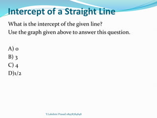
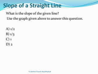
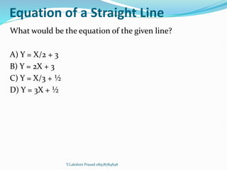
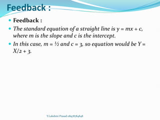
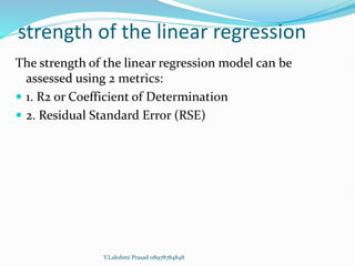
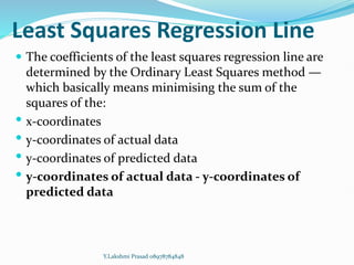
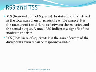
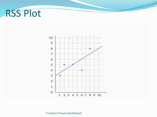
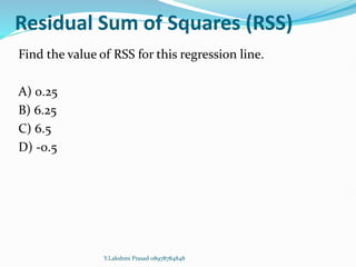
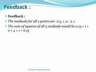
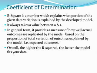
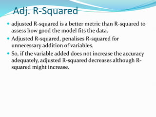
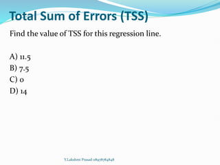
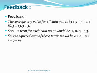
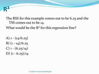
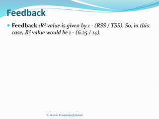
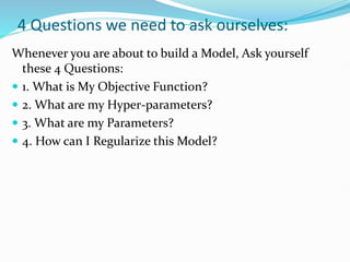
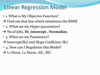
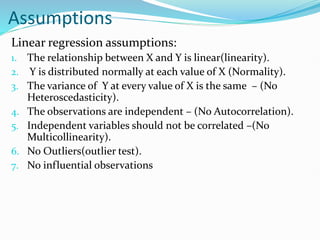
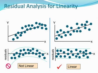
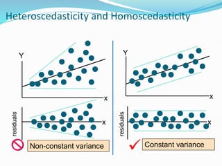
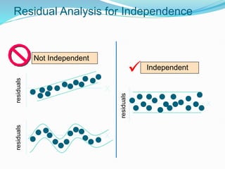
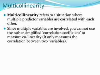
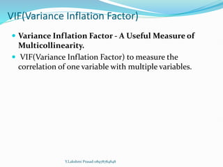
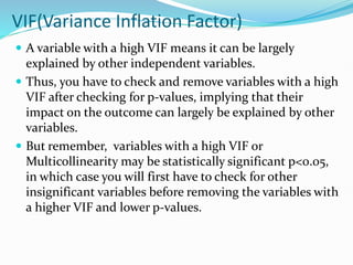
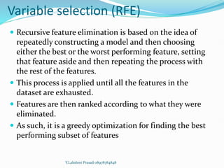
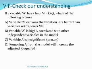
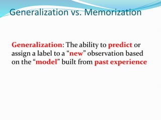
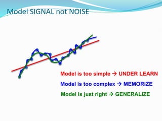
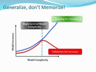
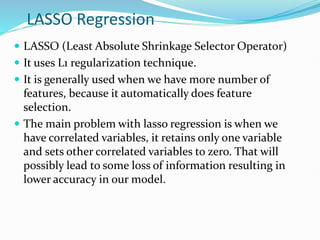
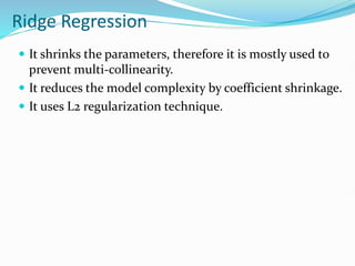
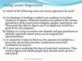
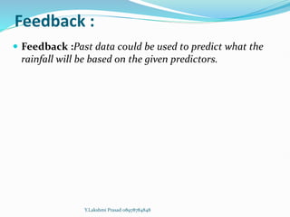
Y.LAKSHMI PRASAD
08978784848
Objectives
1. Describe the Linear Regression Model
2. State the Regression Modeling Steps
3. Explain Ordinary Least Squares
4. Compute Regression Coefficients
5. Understand and check model assumptions
6. Residual sum of squares (RSS) and R² (R-squared)
7. Predict Response Variable
Simple Linear Regression
 The most elementary type of regression model is the
simple linear regression which explains the relationship
between a dependent variable and one independent
variable using a straight line.
 The straight line is plotted on the scatter plot of these
two points.
Y.Lakshmi Prasad 08978784848
Simple Linear regression
In Simple Linear regression, one variable is considered
independent (=predictor) variable (X) and the other the
dependent (=outcome) variable Y (Continuous in nature).
Scatter Plot
Y.Lakshmi Prasad 08978784848
Regression Model
Intercept and Slope
 Since X been given, and we need to predict something
about Y, we require the other 2 parameters those are
slope and intercept.
 Intercept is the value of Y, when X becomes Zero.
 A slope of 2 means that every 1-unit change in X
yields a 2-unit change in Y.
Simple Linear Regression
Y.Lakshmi Prasad 08978784848
Regression Line
Y.Lakshmi Prasad 08978784848
Intercept of a Straight Line
What is the intercept of the given line?
Use the graph given above to answer this question.
A) 0
B) 3
C) 4
D)1/2
Y.Lakshmi Prasad 08978784848
Feedback :
 Feedback :The value of y when x = 0 in the given
straight line is 3.
 So, 3 would be the intercept in this case.
Y.Lakshmi Prasad 08978784848
Slope of a Straight Line
What is the slope of the given line?
Use the graph given above to answer this question.
A) 1/2
B) 1/3
C) 1
D) 2
Y.Lakshmi Prasad 08978784848
Feedback
 Feedback :The slope of any straight line can be
calculated by (y₂ - y₁)/(x₂ - x₁), where (x₁, y₁) and (x₂,
y₂) are any two points through which the given line
passes. This line passes (0,3) and (2, 4); so the slope of
this line would be (4-3/2-0) = ½.
Y.Lakshmi Prasad 08978784848
Equation of a Straight Line
What would be the equation of the given line?
A) Y = X/2 + 3
B) Y = 2X + 3
C) Y = X/3 + ½
D) Y = 3X + ½
Y.Lakshmi Prasad 08978784848
Feedback :
 Feedback :
 The standard equation of a straight line is y = mx + c,
where m is the slope and c is the intercept.
 In this case, m = ½ and c = 3, so equation would be Y =
X/2 + 3.
Y.Lakshmi Prasad 08978784848
strength of the linear regression
The strength of the linear regression model can be
assessed using 2 metrics:
 1. R2 or Coefficient of Determination
 2. Residual Standard Error (RSE)
Y.Lakshmi Prasad 08978784848
Least Squares Regression Line
 The coefficients of the least squares regression line are
determined by the Ordinary Least Squares method —
which basically means minimising the sum of the
squares of the:
 x-coordinates
 y-coordinates of actual data
 y-coordinates of predicted data
 y-coordinates of actual data - y-coordinates of
predicted data
Y.Lakshmi Prasad 08978784848
Feedback :
Feedback :The Ordinary Least Squares method has the
criterion of the minimisation of the sum of squares of
residuals.
Residuals are defined as the difference between the y-
coordinates of actual data and the y-coordinates of
predicted data.
Y.Lakshmi Prasad 08978784848
Best Fit Line
 The best-fit line is found by minimising the expression of
RSS (Residual Sum of Squares) which is equal to the sum
of squares of the residual for each data point in the plot.
 Residuals for any data point is found by subtracting
predicted value of dependent variable from actual value
of dependent variable:
Y.Lakshmi Prasad 08978784848
Residuals
Y.Lakshmi Prasad 08978784848
Best Fit Regression Line
What is the main criterion used to determine the best-
fitting regression line?
A) The line that goes through the most number of points
B) The line that has an equal number of points above it or
below it
C) The line that minimises the sum of squares of
distances of points from the regression line
D) Either B or C (they are same criterion)
Y.Lakshmi Prasad 08978784848
Feedback :
 Answer C: Feedback :The criterion is given by the
Ordinary Least Squares (OLS) method, which states
that the sum of squares of residuals should be
minimum.
Y.Lakshmi Prasad 08978784848
R-Square Formula
RSS - Residual Sum of Squares
 In the previous example of marketing spend (in lakhs)
and sales amount (in crores), let’s assume you get the
same data in different units — marketing spend (in
lakhs) and sales amount (in dollars).
 Do you think there will be any change in the value of
RSS due to change in units in this case (as compared to
the value calculated in the Excel demonstration)?
A) Yes, value of RSS would change because units are
changing.
B) No, value won’t change
C) Can’t say
Y.Lakshmi Prasad 08978784848
Feedback :
 Feedback :The RSS for any regression line is given by
this expression: ∑(yi−yipred)2.
 RSS is the sum of the squared difference between the
actual and the predicted values, and its value will
change if the units change since it has units of y2.
 For example, (140 rupees - 70 rupees)^2 = 4900, whereas
(2 USD - 1 USD)^2 = 1. So value of RSS is different in
both the cases because of different units.
Y.Lakshmi Prasad 08978784848
RSS and TSS
 RSS (Residual Sum of Squares): In statistics, it is defined
as the total sum of error across the whole sample. It is
the measure of the difference between the expected and
the actual output. A small RSS indicates a tight fit of the
model to the data.
 TSS (Total sum of squares): It is the sum of errors of the
data points from mean of response variable.
Y.Lakshmi Prasad 08978784848
RSS Plot
Y.Lakshmi Prasad 08978784848
Residual Sum of Squares (RSS)
Find the value of RSS for this regression line.
A) 0.25
B) 6.25
C) 6.5
D) -0.5
Y.Lakshmi Prasad 08978784848
Feedback :
 Feedback :
 The residuals for all 5 points are -0.5, 1, 0, -2, 1.
 The sum of squares of all 5 residuals would be 0.25 + 1 +
0 + 4 + 1 = 6.25
Y.Lakshmi Prasad 08978784848
Coefficient of Determination
 R-Square is a number which explains what portion of the
given data variation is explained by the developed model.
 It always takes a value between 0 & 1.
 In general term, it provides a measure of how well actual
outcomes are replicated by the model, based on the
proportion of total variation of outcomes explained by
the model, i.e. expected outcomes.
 Overall, the higher the R-squared, the better the model
fits your data.
Adj. R-Squared
 adjusted R-squared is a better metric than R-squared to
assess how good the model fits the data.
 Adjusted R-squared, penalises R-squared for
unnecessary addition of variables.
 So, if the variable added does not increase the accuracy
adequately, adjusted R-squared decreases although R-
squared might increase.
Total Sum of Errors (TSS)
Find the value of TSS for this regression line.
A) 11.5
B) 7.5
C) 0
D) 14
Y.Lakshmi Prasad 08978784848
Feedback :
 Feedback :
 The average of y-value for all data points (3 + 5 + 5 + 4 +
8)/5 = 25/5 = 5.
 So y−¯y term for each data point would be -2, 0, 0, -1, 3.
 So, the squared sum of these terms would be 4 + 0 + 0 +
1 + 9 = 14.
Y.Lakshmi Prasad 08978784848
R²
The RSS for this example comes out to be 6.25 and the
TSS comes out to be 14.
What would be the R² for this regression line?
A) 1 - (14/6.25)
B) (1 - 14)/6.25
C) 1 - (6.25/14)
D) (1 - 6.25)/14
Y.Lakshmi Prasad 08978784848
Feedback
 Feedback :R² value is given by 1 - (RSS / TSS). So, in this
case, R² value would be 1 - (6.25 / 14).
Y.Lakshmi Prasad 08978784848
4 Questions we need to ask ourselves:
Whenever you are about to build a Model, Ask yourself
these 4 Questions:
 1. What is My Objective Function?
 2. What are my Hyper-parameters?
 3. What are my Parameters?
 4. How can I Regularize this Model?
Linear Regression Model
 1. What is My Objective Function?
 Find out that line which minimizes the RMSE
 2. What are my Hyper-parameters?
 No.of Jobs, fit_intercept , Normalize,
 3. What are my Parameters?
 Intercept(B0) and Slope Coeffcient (B1)
 4. How can I Regularize this Model?
 L1 Norm, L2 Norm, AIC, BIC
Multiple linear regression
 Multiple linear regression is a statistical technique to
understand the relationship between one dependent
variable and several independent variables (explanatory
variables).
 The objective of multiple regression is to find a linear
equation that can best determine the value of
dependent variable Y for different values independent
variables in X.
Y.Lakshmi Prasad 08978784848
Multiple linear regression
Y.Lakshmi Prasad 08978784848
Understanding the Regression output
Y.Lakshmi Prasad 08978784848
 We need to understand that not all variables are
used to build a model.
 Some independent variables are insignificant and add
nothing to your understanding of the outcome/
response/ dependent variable.
Y.Lakshmi Prasad 08978784848
standard error
 standard error measures the variability in the estimate
for these coefficients.
 A lower value of standard deviation is good but it is
somewhat relative to the value of the coefficient. E.g.
you can check the standard error of the intercept is
about 0.38, whereas its estimate is 2.6, So, it can be
interpreted that the variability of the intercept is from
2.6±0.38.
 Note that standard error is absolute in nature and so
many a times, it is difficult to judge whether the model
is good or not.
Y.Lakshmi Prasad 08978784848
t-value
 t-value is the ratio of the estimated coefficients to the
standard deviation of the estimated coefficients.
 It measures whether or not the coefficient for this
variable is meaningful for the model.
 It is used to calculate the p-value and the significance
levels which are used for building the final model.
Y.Lakshmi Prasad 08978784848
p-value
 p-value is used for hypothesis testing.
 Here, in regression model building, the null hypothesis
corresponding to each p-value is that the corresponding
independent variable does not impact the dependent
variable.
 The alternate hypothesis is that the corresponding
independent variable impacts the response.
 Now, p-value indicates the probability that the null
hypothesis is true.
 Therefore, a low p-value, i.e. less than 0.05, indicates
that you can reject the null hypothesis.
Y.Lakshmi Prasad 08978784848
P-Value
Y.Lakshmi Prasad 08978784848
Assumptions
Linear regression assumptions:
1. The relationship between X and Y is linear(linearity).
2. Y is distributed normally at each value of X (Normality).
3. The variance of Y at every value of X is the same – (No
Heteroscedasticity).
4. The observations are independent – (No Autocorrelation).
5. Independent variables should not be correlated –(No
Multicollinearity).
6. No Outliers(outlier test).
7. No influential observations
Residual Analysis for Linearity
Not Linear Linear

x
residuals
x
Y
x
Y
x
residuals
Heteroscedasticity and Homoscedasticity
Non-constant variance  Constant variance
x x
Y
x x
Y
residuals
residuals
Residual Analysis for Independence
Not Independent
Independent
X
X
residuals
residuals
X
residuals

Gradient Descent
Multicollinearity
 Multicollinearity refers to a situation where
multiple predictor variables are correlated with each
other.
 Since multiple variables are involved, you cannot use
the rather simplified 'correlation coefficient' to
measure co-linearity (it only measures the
correlation between two variables).
Multicollinearity
 Since one of the major goal of linear regression is
identifying the important explanatory variables, it is
important to assess the impact of each and then keep
those which have a significant impact on the outcome.
This is the major issue with Multicollinearity.
 Multicollinearity makes it difficult to assess the effect
of individual predictors.
Y.Lakshmi Prasad 08978784848
Multicollinearity
 A simple way to detect Multicollinearity is to look at the
correlation matrix.
 We can use Heat map to find the Multicollinearity.
 The statistical test VIF(Variance Inflation Factor) is often
used to detect Multicollinearity.
Y.Lakshmi Prasad 08978784848
VIF(Variance Inflation Factor)
 Variance Inflation Factor - A Useful Measure of
Multicollinearity.
 VIF(Variance Inflation Factor) to measure the
correlation of one variable with multiple variables.
Y.Lakshmi Prasad 08978784848
VIF(Variance Inflation Factor)
 A variable with a high VIF means it can be largely
explained by other independent variables.
 Thus, you have to check and remove variables with a high
VIF after checking for p-values, implying that their
impact on the outcome can largely be explained by other
variables.
 But remember, variables with a high VIF or
Multicollinearity may be statistically significant p<0.05,
in which case you will first have to check for other
insignificant variables before removing the variables with
a higher VIF and lower p-values.
Variable selection (RFE)
 Recursive feature elimination is based on the idea of
repeatedly constructing a model and then choosing
either the best or the worst performing feature, setting
that feature aside and then repeating the process with
the rest of the features.
 This process is applied until all the features in the
dataset are exhausted.
 Features are then ranked according to what they were
eliminated.
 As such, it is a greedy optimization for finding the best
performing subset of features
Y.Lakshmi Prasad 08978784848
VIF-Check our understanding
If a variable “A” has a high VIF (>5), which of the
following is true?
A) Variable “A” explains the variation in Y better than
variables with a lower VIF
B) Variable “A” is highly correlated with other
independent variables in the model
C) Variable A is insignificant (p>0.05)
D) Removing A from the model will increase the
adjusted R-squared
Y.Lakshmi Prasad 08978784848
linear regression model building process:
 Once you understood the business objective, you prepared
the data, followed by EDA and the division of data into
training and test datasets.
 The next step was the selection of variables for the creation
of the model. Variable selection is critical because you
cannot just include all the variables in the model; otherwise,
you run the risk of including insignificant variables too.
 This is RFE can be used to quickly shortlist some variables
which are significant to save time.
 However, these significant independent variables might be
related to each other. This is where you need to check for
multicollinearity amongst variables using variance inflation
factor (VIF) and remove variables with high VIF and low
significance (p>0.05).
Y.Lakshmi Prasad 08978784848
linear regression model building process:
 The variables with a high VIF or multi-collinearity may
be statistically significant or p<0.05, in which case you
will first have to check for other insignificant variables
(p>0.05) before removing the variables with a higher
VIF and lower p-values.
 Continue removing the variables until all variables are
significant or p<0.05, and have low VIFs.
 Finally you arrive at a model where all variables are
significant and there is no threat of multi-collinearity.
 The final step is to check the model accuracy on the
testing data.
Y.Lakshmi Prasad 08978784848
Model Building- Test
An analyst observes a positive relationship between digital
marketing expenses and online sales for a firm. However,
she intuitively feels that she should add an additional
independent variable, one which has a high correlation with
marketing expenses.
If the analyst adds this independent variable to the model,
which of the following could happen?
More than one choices could be correct.(Find out Both)
A) The model’s R-squared will decrease
B) The model’s adjusted R-squared could decrease
C) The Beta-coefficient for predictor - digital marketing
expenses will remain same
D) The relationship between marketing expenses and sales
can become insignificant
Y.Lakshmi Prasad 08978784848
Feedback
 Feedback :Adjusted R-squared could decrease if the
variable does not add much to the model, to explain
Online Sales.
 Feedback :The relation between marketing expenses
and sales can become insignificant with the addition of
a new variable.
Y.Lakshmi Prasad 08978784848
Dummy Variables
Suppose you need to build a model on a data set which
contains 2 categorical variables with 2 and 4 levels
respectively.
How many dummy variables should you create for model
building?
A) 6
B) 4
C) 2
D) 8
Y.Lakshmi Prasad 08978784848
Feedback :
 Since n-1 dummy variables can be used to describe a
variable with n levels, you will get 1 dummy variable for
the variable with two levels, and 3 dummy variables for
the variable with 4 levels.
Y.Lakshmi Prasad 08978784848
Data Partition
 Whenever I am Building a Model, I want my model to
predict the unseen(new) cases. To facilitate this, we
split the given dataset in to 2 datasets 1. Training and 2.
Validation.
 1. Training Dataset: is to Build the Model
 2. Validation Dataset: is to Evaluate the Model.
Model Validation
 It is desired that the R-squared between the predicted
value and the actual value in the test set should be high.
 In general, it is desired that the R-squared on the test
data be high, and as similar to the R-squared on the
training set as possible.
 We should note that R-squared is only one of the metric
among many other metrics to assess accuracy in a linear
regression model.
Y.Lakshmi Prasad 08978784848
Generalization: The ability to predict or
assign a label to a “new” observation based
on the “model” built from past experience
Generalization vs. Memorization
Model SIGNAL not NOISE
Model is too simple  UNDER LEARN
Model is too complex  MEMORIZE
Model is just right  GENERALIZE
Generalize, don’t Memorize!
Model Complexity
Model
Accuracy
Training Set Accuracy
Validation Set Accuracy
Right Level of Model
Complexity
Overfitting
 In multivariate modeling, you can get highly significant
but meaningless results if you put too many predictors
in the model.
 The model is fit perfectly to the training data, but has
no predictive ability in a new sample (Validation Data).
LASSO Regression
 LASSO (Least Absolute Shrinkage Selector Operator)
 It uses L1 regularization technique.
 It is generally used when we have more number of
features, because it automatically does feature
selection.
 The main problem with lasso regression is when we
have correlated variables, it retains only one variable
and sets other correlated variables to zero. That will
possibly lead to some loss of information resulting in
lower accuracy in our model.
Ridge Regression
 It shrinks the parameters, therefore it is mostly used to
prevent multi-collinearity.
 It reduces the model complexity by coefficient shrinkage.
 It uses L2 regularization technique.
Using Linear Regression
In which of the following cases can linear regression be used?
A) An Institute is looking to admit new students in its Data
Analytics Program. Potential students are asked to fill various
parameters such as previous company, grades, experience, etc.
They need this data to figure out if an applicant would be a
good fit for the program.
B) Flipkart is trying to analyse user details and past purchases to
identify segments where users can be targeted for
advertisements.
C) A researcher wishes to find out the amount of rainfall on a
given day, given that pressure, temperature and wind
conditions are known.
D) A start-up is analysing the data of potential customers. They
need to figure out which people they should reach out for a
sales pitch.
Y.Lakshmi Prasad 08978784848
Feedback :
 Feedback :Past data could be used to predict what the
rainfall will be based on the given predictors.
Y.Lakshmi Prasad 08978784848
Questions?
Y.Lakshmi Prasad 08978784848

Linear Regression in Machine Learning YLP

  • 1.
  • 2.
    Objectives 1. Describe theLinear Regression Model 2. State the Regression Modeling Steps 3. Explain Ordinary Least Squares 4. Compute Regression Coefficients 5. Understand and check model assumptions 6. Residual sum of squares (RSS) and R² (R-squared) 7. Predict Response Variable
  • 3.
    Simple Linear Regression The most elementary type of regression model is the simple linear regression which explains the relationship between a dependent variable and one independent variable using a straight line.  The straight line is plotted on the scatter plot of these two points. Y.Lakshmi Prasad 08978784848
  • 4.
    Simple Linear regression InSimple Linear regression, one variable is considered independent (=predictor) variable (X) and the other the dependent (=outcome) variable Y (Continuous in nature).
  • 5.
  • 6.
  • 7.
    Intercept and Slope Since X been given, and we need to predict something about Y, we require the other 2 parameters those are slope and intercept.  Intercept is the value of Y, when X becomes Zero.  A slope of 2 means that every 1-unit change in X yields a 2-unit change in Y.
  • 8.
  • 9.
  • 10.
    Intercept of aStraight Line What is the intercept of the given line? Use the graph given above to answer this question. A) 0 B) 3 C) 4 D)1/2 Y.Lakshmi Prasad 08978784848
  • 11.
    Feedback :  Feedback:The value of y when x = 0 in the given straight line is 3.  So, 3 would be the intercept in this case. Y.Lakshmi Prasad 08978784848
  • 12.
    Slope of aStraight Line What is the slope of the given line? Use the graph given above to answer this question. A) 1/2 B) 1/3 C) 1 D) 2 Y.Lakshmi Prasad 08978784848
  • 13.
    Feedback  Feedback :Theslope of any straight line can be calculated by (y₂ - y₁)/(x₂ - x₁), where (x₁, y₁) and (x₂, y₂) are any two points through which the given line passes. This line passes (0,3) and (2, 4); so the slope of this line would be (4-3/2-0) = ½. Y.Lakshmi Prasad 08978784848
  • 14.
    Equation of aStraight Line What would be the equation of the given line? A) Y = X/2 + 3 B) Y = 2X + 3 C) Y = X/3 + ½ D) Y = 3X + ½ Y.Lakshmi Prasad 08978784848
  • 15.
    Feedback :  Feedback:  The standard equation of a straight line is y = mx + c, where m is the slope and c is the intercept.  In this case, m = ½ and c = 3, so equation would be Y = X/2 + 3. Y.Lakshmi Prasad 08978784848
  • 16.
    strength of thelinear regression The strength of the linear regression model can be assessed using 2 metrics:  1. R2 or Coefficient of Determination  2. Residual Standard Error (RSE) Y.Lakshmi Prasad 08978784848
  • 17.
    Least Squares RegressionLine  The coefficients of the least squares regression line are determined by the Ordinary Least Squares method — which basically means minimising the sum of the squares of the:  x-coordinates  y-coordinates of actual data  y-coordinates of predicted data  y-coordinates of actual data - y-coordinates of predicted data Y.Lakshmi Prasad 08978784848
  • 18.
    Feedback : Feedback :TheOrdinary Least Squares method has the criterion of the minimisation of the sum of squares of residuals. Residuals are defined as the difference between the y- coordinates of actual data and the y-coordinates of predicted data. Y.Lakshmi Prasad 08978784848
  • 19.
    Best Fit Line The best-fit line is found by minimising the expression of RSS (Residual Sum of Squares) which is equal to the sum of squares of the residual for each data point in the plot.  Residuals for any data point is found by subtracting predicted value of dependent variable from actual value of dependent variable: Y.Lakshmi Prasad 08978784848
  • 20.
  • 21.
    Best Fit RegressionLine What is the main criterion used to determine the best- fitting regression line? A) The line that goes through the most number of points B) The line that has an equal number of points above it or below it C) The line that minimises the sum of squares of distances of points from the regression line D) Either B or C (they are same criterion) Y.Lakshmi Prasad 08978784848
  • 22.
    Feedback :  AnswerC: Feedback :The criterion is given by the Ordinary Least Squares (OLS) method, which states that the sum of squares of residuals should be minimum. Y.Lakshmi Prasad 08978784848
  • 23.
  • 24.
    RSS - ResidualSum of Squares  In the previous example of marketing spend (in lakhs) and sales amount (in crores), let’s assume you get the same data in different units — marketing spend (in lakhs) and sales amount (in dollars).  Do you think there will be any change in the value of RSS due to change in units in this case (as compared to the value calculated in the Excel demonstration)? A) Yes, value of RSS would change because units are changing. B) No, value won’t change C) Can’t say Y.Lakshmi Prasad 08978784848
  • 25.
    Feedback :  Feedback:The RSS for any regression line is given by this expression: ∑(yi−yipred)2.  RSS is the sum of the squared difference between the actual and the predicted values, and its value will change if the units change since it has units of y2.  For example, (140 rupees - 70 rupees)^2 = 4900, whereas (2 USD - 1 USD)^2 = 1. So value of RSS is different in both the cases because of different units. Y.Lakshmi Prasad 08978784848
  • 26.
    RSS and TSS RSS (Residual Sum of Squares): In statistics, it is defined as the total sum of error across the whole sample. It is the measure of the difference between the expected and the actual output. A small RSS indicates a tight fit of the model to the data.  TSS (Total sum of squares): It is the sum of errors of the data points from mean of response variable. Y.Lakshmi Prasad 08978784848
  • 27.
  • 28.
    Residual Sum ofSquares (RSS) Find the value of RSS for this regression line. A) 0.25 B) 6.25 C) 6.5 D) -0.5 Y.Lakshmi Prasad 08978784848
  • 29.
    Feedback :  Feedback:  The residuals for all 5 points are -0.5, 1, 0, -2, 1.  The sum of squares of all 5 residuals would be 0.25 + 1 + 0 + 4 + 1 = 6.25 Y.Lakshmi Prasad 08978784848
  • 30.
    Coefficient of Determination R-Square is a number which explains what portion of the given data variation is explained by the developed model.  It always takes a value between 0 & 1.  In general term, it provides a measure of how well actual outcomes are replicated by the model, based on the proportion of total variation of outcomes explained by the model, i.e. expected outcomes.  Overall, the higher the R-squared, the better the model fits your data.
  • 31.
    Adj. R-Squared  adjustedR-squared is a better metric than R-squared to assess how good the model fits the data.  Adjusted R-squared, penalises R-squared for unnecessary addition of variables.  So, if the variable added does not increase the accuracy adequately, adjusted R-squared decreases although R- squared might increase.
  • 32.
    Total Sum ofErrors (TSS) Find the value of TSS for this regression line. A) 11.5 B) 7.5 C) 0 D) 14 Y.Lakshmi Prasad 08978784848
  • 33.
    Feedback :  Feedback:  The average of y-value for all data points (3 + 5 + 5 + 4 + 8)/5 = 25/5 = 5.  So y−¯y term for each data point would be -2, 0, 0, -1, 3.  So, the squared sum of these terms would be 4 + 0 + 0 + 1 + 9 = 14. Y.Lakshmi Prasad 08978784848
  • 34.
    R² The RSS forthis example comes out to be 6.25 and the TSS comes out to be 14. What would be the R² for this regression line? A) 1 - (14/6.25) B) (1 - 14)/6.25 C) 1 - (6.25/14) D) (1 - 6.25)/14 Y.Lakshmi Prasad 08978784848
  • 35.
    Feedback  Feedback :R²value is given by 1 - (RSS / TSS). So, in this case, R² value would be 1 - (6.25 / 14). Y.Lakshmi Prasad 08978784848
  • 36.
    4 Questions weneed to ask ourselves: Whenever you are about to build a Model, Ask yourself these 4 Questions:  1. What is My Objective Function?  2. What are my Hyper-parameters?  3. What are my Parameters?  4. How can I Regularize this Model?
  • 37.
    Linear Regression Model 1. What is My Objective Function?  Find out that line which minimizes the RMSE  2. What are my Hyper-parameters?  No.of Jobs, fit_intercept , Normalize,  3. What are my Parameters?  Intercept(B0) and Slope Coeffcient (B1)  4. How can I Regularize this Model?  L1 Norm, L2 Norm, AIC, BIC
  • 38.
    Multiple linear regression Multiple linear regression is a statistical technique to understand the relationship between one dependent variable and several independent variables (explanatory variables).  The objective of multiple regression is to find a linear equation that can best determine the value of dependent variable Y for different values independent variables in X. Y.Lakshmi Prasad 08978784848
  • 39.
  • 40.
    Understanding the Regressionoutput Y.Lakshmi Prasad 08978784848
  • 41.
     We needto understand that not all variables are used to build a model.  Some independent variables are insignificant and add nothing to your understanding of the outcome/ response/ dependent variable. Y.Lakshmi Prasad 08978784848
  • 42.
    standard error  standarderror measures the variability in the estimate for these coefficients.  A lower value of standard deviation is good but it is somewhat relative to the value of the coefficient. E.g. you can check the standard error of the intercept is about 0.38, whereas its estimate is 2.6, So, it can be interpreted that the variability of the intercept is from 2.6±0.38.  Note that standard error is absolute in nature and so many a times, it is difficult to judge whether the model is good or not. Y.Lakshmi Prasad 08978784848
  • 43.
    t-value  t-value isthe ratio of the estimated coefficients to the standard deviation of the estimated coefficients.  It measures whether or not the coefficient for this variable is meaningful for the model.  It is used to calculate the p-value and the significance levels which are used for building the final model. Y.Lakshmi Prasad 08978784848
  • 44.
    p-value  p-value isused for hypothesis testing.  Here, in regression model building, the null hypothesis corresponding to each p-value is that the corresponding independent variable does not impact the dependent variable.  The alternate hypothesis is that the corresponding independent variable impacts the response.  Now, p-value indicates the probability that the null hypothesis is true.  Therefore, a low p-value, i.e. less than 0.05, indicates that you can reject the null hypothesis. Y.Lakshmi Prasad 08978784848
  • 45.
  • 46.
    Assumptions Linear regression assumptions: 1.The relationship between X and Y is linear(linearity). 2. Y is distributed normally at each value of X (Normality). 3. The variance of Y at every value of X is the same – (No Heteroscedasticity). 4. The observations are independent – (No Autocorrelation). 5. Independent variables should not be correlated –(No Multicollinearity). 6. No Outliers(outlier test). 7. No influential observations
  • 47.
    Residual Analysis forLinearity Not Linear Linear  x residuals x Y x Y x residuals
  • 48.
    Heteroscedasticity and Homoscedasticity Non-constantvariance  Constant variance x x Y x x Y residuals residuals
  • 49.
    Residual Analysis forIndependence Not Independent Independent X X residuals residuals X residuals 
  • 50.
  • 51.
    Multicollinearity  Multicollinearity refersto a situation where multiple predictor variables are correlated with each other.  Since multiple variables are involved, you cannot use the rather simplified 'correlation coefficient' to measure co-linearity (it only measures the correlation between two variables).
  • 52.
    Multicollinearity  Since oneof the major goal of linear regression is identifying the important explanatory variables, it is important to assess the impact of each and then keep those which have a significant impact on the outcome. This is the major issue with Multicollinearity.  Multicollinearity makes it difficult to assess the effect of individual predictors. Y.Lakshmi Prasad 08978784848
  • 53.
    Multicollinearity  A simpleway to detect Multicollinearity is to look at the correlation matrix.  We can use Heat map to find the Multicollinearity.  The statistical test VIF(Variance Inflation Factor) is often used to detect Multicollinearity. Y.Lakshmi Prasad 08978784848
  • 54.
    VIF(Variance Inflation Factor) Variance Inflation Factor - A Useful Measure of Multicollinearity.  VIF(Variance Inflation Factor) to measure the correlation of one variable with multiple variables. Y.Lakshmi Prasad 08978784848
  • 55.
    VIF(Variance Inflation Factor) A variable with a high VIF means it can be largely explained by other independent variables.  Thus, you have to check and remove variables with a high VIF after checking for p-values, implying that their impact on the outcome can largely be explained by other variables.  But remember, variables with a high VIF or Multicollinearity may be statistically significant p<0.05, in which case you will first have to check for other insignificant variables before removing the variables with a higher VIF and lower p-values.
  • 56.
    Variable selection (RFE) Recursive feature elimination is based on the idea of repeatedly constructing a model and then choosing either the best or the worst performing feature, setting that feature aside and then repeating the process with the rest of the features.  This process is applied until all the features in the dataset are exhausted.  Features are then ranked according to what they were eliminated.  As such, it is a greedy optimization for finding the best performing subset of features Y.Lakshmi Prasad 08978784848
  • 57.
    VIF-Check our understanding Ifa variable “A” has a high VIF (>5), which of the following is true? A) Variable “A” explains the variation in Y better than variables with a lower VIF B) Variable “A” is highly correlated with other independent variables in the model C) Variable A is insignificant (p>0.05) D) Removing A from the model will increase the adjusted R-squared Y.Lakshmi Prasad 08978784848
  • 58.
    linear regression modelbuilding process:  Once you understood the business objective, you prepared the data, followed by EDA and the division of data into training and test datasets.  The next step was the selection of variables for the creation of the model. Variable selection is critical because you cannot just include all the variables in the model; otherwise, you run the risk of including insignificant variables too.  This is RFE can be used to quickly shortlist some variables which are significant to save time.  However, these significant independent variables might be related to each other. This is where you need to check for multicollinearity amongst variables using variance inflation factor (VIF) and remove variables with high VIF and low significance (p>0.05). Y.Lakshmi Prasad 08978784848
  • 59.
    linear regression modelbuilding process:  The variables with a high VIF or multi-collinearity may be statistically significant or p<0.05, in which case you will first have to check for other insignificant variables (p>0.05) before removing the variables with a higher VIF and lower p-values.  Continue removing the variables until all variables are significant or p<0.05, and have low VIFs.  Finally you arrive at a model where all variables are significant and there is no threat of multi-collinearity.  The final step is to check the model accuracy on the testing data. Y.Lakshmi Prasad 08978784848
  • 60.
    Model Building- Test Ananalyst observes a positive relationship between digital marketing expenses and online sales for a firm. However, she intuitively feels that she should add an additional independent variable, one which has a high correlation with marketing expenses. If the analyst adds this independent variable to the model, which of the following could happen? More than one choices could be correct.(Find out Both) A) The model’s R-squared will decrease B) The model’s adjusted R-squared could decrease C) The Beta-coefficient for predictor - digital marketing expenses will remain same D) The relationship between marketing expenses and sales can become insignificant Y.Lakshmi Prasad 08978784848
  • 61.
    Feedback  Feedback :AdjustedR-squared could decrease if the variable does not add much to the model, to explain Online Sales.  Feedback :The relation between marketing expenses and sales can become insignificant with the addition of a new variable. Y.Lakshmi Prasad 08978784848
  • 62.
    Dummy Variables Suppose youneed to build a model on a data set which contains 2 categorical variables with 2 and 4 levels respectively. How many dummy variables should you create for model building? A) 6 B) 4 C) 2 D) 8 Y.Lakshmi Prasad 08978784848
  • 63.
    Feedback :  Sincen-1 dummy variables can be used to describe a variable with n levels, you will get 1 dummy variable for the variable with two levels, and 3 dummy variables for the variable with 4 levels. Y.Lakshmi Prasad 08978784848
  • 64.
    Data Partition  WheneverI am Building a Model, I want my model to predict the unseen(new) cases. To facilitate this, we split the given dataset in to 2 datasets 1. Training and 2. Validation.  1. Training Dataset: is to Build the Model  2. Validation Dataset: is to Evaluate the Model.
  • 65.
    Model Validation  Itis desired that the R-squared between the predicted value and the actual value in the test set should be high.  In general, it is desired that the R-squared on the test data be high, and as similar to the R-squared on the training set as possible.  We should note that R-squared is only one of the metric among many other metrics to assess accuracy in a linear regression model. Y.Lakshmi Prasad 08978784848
  • 66.
    Generalization: The abilityto predict or assign a label to a “new” observation based on the “model” built from past experience Generalization vs. Memorization
  • 67.
    Model SIGNAL notNOISE Model is too simple  UNDER LEARN Model is too complex  MEMORIZE Model is just right  GENERALIZE
  • 68.
    Generalize, don’t Memorize! ModelComplexity Model Accuracy Training Set Accuracy Validation Set Accuracy Right Level of Model Complexity
  • 69.
    Overfitting  In multivariatemodeling, you can get highly significant but meaningless results if you put too many predictors in the model.  The model is fit perfectly to the training data, but has no predictive ability in a new sample (Validation Data).
  • 70.
    LASSO Regression  LASSO(Least Absolute Shrinkage Selector Operator)  It uses L1 regularization technique.  It is generally used when we have more number of features, because it automatically does feature selection.  The main problem with lasso regression is when we have correlated variables, it retains only one variable and sets other correlated variables to zero. That will possibly lead to some loss of information resulting in lower accuracy in our model.
  • 71.
    Ridge Regression  Itshrinks the parameters, therefore it is mostly used to prevent multi-collinearity.  It reduces the model complexity by coefficient shrinkage.  It uses L2 regularization technique.
  • 72.
    Using Linear Regression Inwhich of the following cases can linear regression be used? A) An Institute is looking to admit new students in its Data Analytics Program. Potential students are asked to fill various parameters such as previous company, grades, experience, etc. They need this data to figure out if an applicant would be a good fit for the program. B) Flipkart is trying to analyse user details and past purchases to identify segments where users can be targeted for advertisements. C) A researcher wishes to find out the amount of rainfall on a given day, given that pressure, temperature and wind conditions are known. D) A start-up is analysing the data of potential customers. They need to figure out which people they should reach out for a sales pitch. Y.Lakshmi Prasad 08978784848
  • 73.
    Feedback :  Feedback:Past data could be used to predict what the rainfall will be based on the given predictors. Y.Lakshmi Prasad 08978784848
  • 74.