
More Related Content
What's hot
What's hot (20)
Viewers also liked
Viewers also liked (18)
Similar to Em03 t
Similar to Em03 t (20)
More from nahomyitbarek
More from nahomyitbarek (20)
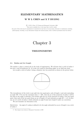
Em03 t
- 1. ELEMENTARY MATHEMATICS W W L CHEN and X T DUONG c W W L Chen, X T Duong and Macquarie University, 1999. This work is available free, in the hope that it will be useful. Any part of this work may be reproduced or transmitted in any form or by any means, electronic or mechanical, including photocopying, recording, or any information storage and retrieval system, with or without permission from the authors. Chapter 3 TRIGONOMETRY 3.1. Radian and Arc Length The number π plays a central role in the study of trigonometry. We all know that a circle of radius 1 has area π and circumference 2π. It is also very useful in describing angles, as we shall now show. Let us split a circle of radius 1 along a diameter into two semicircles as shown in the picture below. The circumference of the circle is now split into two equal parts, each of length π and each suntending an angle 180◦ . If we use the convention that π = 180◦ , then the arc of the semicircle of radius 1 will be the same as the angle it subtends. If we further split the arc of the semicircle of radius 1 into two equal parts, then each of the two parts forms an arc of length π/2 and subtends an angle 90◦ = π/2. In fact, any arc of a circle of radius 1 which subtends an angle θ must have length θ under our convention. We now formalize our discussion so far. Definition. An angle of 1 radian is defined to be the angle subtended by an arc of length 1 on a circle of radius 1. † This chapter was written at Macquarie University in 1999.
- 2. 3–2 W W L Chen and X T Duong : Elementary Mathematics Remarks. (1) Very often, the term radian is omitted when we discuss angles. We simply refer to an angle 1 or an angle π, rather than an angle of 1 radian or an angle of π radian. (2) Simple calculation shows that 1 radian is equal to (180/π)◦ = 57.2957795 . . .◦ . Similarly, we can show that 1◦ is equal to (π/180) radian = 0.01745329 . . . radian. In fact, since π is irrational, the digits do not terminate or repeat. (3) We observe the following special values: π π π π = 30◦ , = 45◦ , = 60◦ , = 90◦ , π = 180◦ , 2π = 360◦ . 6 4 3 2 Consider now a circle of radius r and an angle θ given in radian, as shown in the picture below. rθ θ r Clearly the length s of the arc which subtends the angle θ satisfies s = rθ, while the area A of the sector satisfies θ 1 A = πr2 × = r2 θ. 2π 2 Note that πr2 is equal to the area inside the circle, while θ/2π is the proportion of the area in question. 3.2. The Trigonometric Functions Consider the xy-plane, together with a circle of radius 1 and centred at the origin (0, 0). Suppose that θ is an angle measured anticlockwise from the positive x-axis, and the point (x, y) on the circle is as shown in the picture below. y 1 θ x We define cos θ = x and sin θ = y. Furthermore, we define sin θ y cos θ x 1 1 1 1 tan θ = = , cot θ = = , sec θ = = and csc θ = = . cos θ x sin θ y cos θ x sin θ y
- 3. Chapter 3 : Trigonometry 3–3 Remarks. (1) Note that tan θ and sec θ are defined only when cos θ = 0, and that cot θ and csc θ are defined only when sin θ = 0. (2) It is a good habit to always measure an angle from the positive x-axis, using the convention that positive angles are measured anticlockwise and negative angles are measured clockwise, as illustrated below. 1 3π 4 -1 π 2 (3) We then observe that horizontal side vertical side cos θ = and sin θ = , hypothenuse hypothenuse as well as vertical side horizontal side tan θ = and cot θ = , horizontal side vertical side with the convention that > 0 (to the right of the (vertical) y-axis), horizontal side < 0 (to the left of the (vertical) y-axis), and > 0 (above the (horizontal) x-axis), vertical side < 0 (below the (horizontal) x-axis), while hypothenuse > 0 (always). (4) It is also useful to remember the CAST rule concerning sine, cosine and tangent. S (sin > 0) A (all > 0) T (tan > 0) C (cos > 0) PYTHAGOREAN IDENTITIES. For every value θ ∈ R for which the trigonometric functions in question are defined, we have (a) cos2 θ + sin2 θ = 1; (b) 1 + tan2 θ = sec2 θ; and (c) 1 + cot2 θ = csc2 θ.
- 4. 3–4 W W L Chen and X T Duong : Elementary Mathematics Proof. Note that (a) follows from the classical Pythagoras’s theorem. If cos θ = 0, then dividing both sides of (a) by cos2 θ gives (b). If sin θ = 0, then dividing both sides of (a) by sin2 θ gives (c). ♣ We sketch the graphs of the functions y = sin x, y = cos x and y = tan x for −2π ≤ x ≤ 2π below: y 1 y = sin x x -2π -π π 2π -1 y 1 y = cos x x -2π -π π 2π -1 y y = tan x x -2π -π π 2π We shall use these graphs to make some observations about trigonometric functions.
- 5. Chapter 3 : Trigonometry 3–5 PROPERTIES OF TRIGONOMETRIC FUNCTIONS. (a) The functions sin x and cos x are periodic with period 2π. More precisely, for every x ∈ R, we have sin(x + 2π) = sin x and cos(x + 2π) = cos x. (b) The functions tan x and cot x are periodic with period π. More precisely, for every x ∈ R for which the trigonometric function in question is defined, we have tan(x + π) = tan x and cot(x + π) = cot x. (c) The function sin x is an odd function, and the function cos x is an even function. More precisely, for every x ∈ R, we have sin(−x) = − sin x and cos(−x) = cos x. (d) The functions tan x and cot x are odd functions. More precisely, for every x ∈ R for which the trigonometric function in question is defined, we have tan(−x) = − tan x and cot(−x) = − cot x. (e) For every x ∈ R, we have sin(x + π) = − sin x and cos(x + π) = − cos x. (f) For every x ∈ R, we have sin(π − x) = sin x and cos(π − x) = − cos x. (g) For every x ∈ R for which the trigonometric function in question is defined, we have tan(π − x) = − tan x and cot(π − x) = − cot x. (h) For every x ∈ R, we have π π sin x + = cos x and cos x + = − sin x. 2 2 (i) For every x ∈ R, we have π π sin − x = cos x and cos − x = sin x. 2 2 (j) For every x ∈ R for which the trigonometric functions in question are defined, we have π π tan x + = − cot x and cot x + = − tan x. 2 2 (k) For every x ∈ R for which the trigonometric function in question is defined, we have π π tan − x = cot x and cot − x = tan x. 2 2 Remark. There is absolutely no need to remember any of these properties! We shall discuss later some trigonometric identities which will give all the above as special cases.
- 6. 3–6 W W L Chen and X T Duong : Elementary Mathematics Example 3.2.1. Consider the following picture. 1 π/6 Clearly the triangle shown is an equilateral triangle, with all three sides of equal length. It is also clear that sin(π/6) is half the length of the vertical side. It follows that we must have sin(π/6) = 1/2. To find the precise value for cos(π/6), we first observe that cos(π/6) > 0. On the other hand, it follows from the √ first of the Pythagorean identities that cos2 (π/6) = 3/4. Hence cos(π/6) = 3/2. We can then deduce √ that tan(π/6) = 1/ 3. √ Example 3.2.2. We have tan(13π/6) = tan(7π/6) = tan(π/6) = 1/ 3. Note that we have used part (b) of the Properties of trigonometric functions, as well as the result from Example 3.2.1. Example 3.2.3. Consider the following picture. -π/3 1 Clearly the triangle shown is an equilateral triangle, with all three sides of equal length. It is also clear that cos(−π/3) is half the length the horizontal side. It follows that we must have cos(−π/3) = 1/2. To find the precise value for sin(−π/3), we first observe that sin(−π/3) < 0. On the other hand, follows from the first of the Pythagorean identities that sin2 (−π/3) = 3/4. Hence sin(−π/3) = it √ − 3/2. Alternatively, we can deduce from Example 3.2.1 by using parts (c) and (i) of the Properties of
- 7. Chapter 3 : Trigonometry 3–7 trigonometric functions that π π π π π 1 cos − = cos = sin − = sin = 3 3 2 3 6 2 and √ π π π π π 3 sin − = − sin = − cos − = − cos = − . 3 3 2 3 6 2 √ We can then deduce that tan(−π/3) = − 3. Example 3.2.4. Consider the following picture. 5 π/4 1 Clearly the triangle shown is a right-angled triangle with the two shorter sides of equal length and hypothenuse of length 1. It is also clear that sin(5π/4) is the length of the vertical side, with a − sign attached as it is below the horizontal axis. On the other hand, it is also clear that cos(5π/4) is the length of the horizontal side, again with a − sign attached as it is left of the vertical axis. It follows from Pythagoras’s theorem that sin(5π/4) = cos(5π/4) = y, where y < 0 and y 2 + y 2 = 1. Clearly √ y = −1/ 2. We can then deduce that tan(5π/4) = 1. √ Example 3.2.5. To find all the solutions of the equation sin x = −1/ 2 in the interval 0 ≤ x < 2π, we consider the following picture. 7 π/4 1 1
- 8. 3–8 W W L Chen and X T Duong : Elementary Mathematics Using Pythagoras’s theorem, it is easy to see that the two triangles shown both have horizontal side of √ length 1/ 2, the same as the length of their vertical sides. Clearly x = 5π/4 or x = 7π/4. Example 3.2.6. Suppose that we wish to find all the solutions of the equation cos2 x = 1/4 in the interval −π/2 < x ≤ π. Observe first of all that either cos x = 1/2 or cos x = −1/2. We consider the following picture. 1 1 2 π/3 - π/3 1 Using Pythagoras’s theorem, it is easy to see that the three triangles shown both have vertical side of √ length 3/2. Clearly x = −π/3, x = π/3 or x = 2π/3. Example 3.2.7. Convince yourself that the only two solutions of the equation cos2 x = 1 in the interval 0 ≤ x < 2π are x = 0 and x = π. √ Example 3.2.8. To find all the solutions of the equation tan x = 3 in the interval 0 ≤ x < 2π, we consider the following picture. 1 4π/3 1 Since tan x > 0, it follows from the CAST rule that we can restrict our attention to the first and third quadrants. It is easy to check that the two triangles shown have horizontal sides of length 1/2 and √ vertical sides of length 3/2. Clearly x = π/3 or x = 4π/3.
- 9. Chapter 3 : Trigonometry 3–9 Example 3.2.9. Suppose that we wish to find all the solutions of the equation √ 2 x = 1/3 in the √ tan interval 0 ≤ x ≤ 3π/2. Observe first of all that either tan x = 1/ 3 or tan x = −1/ 3. We consider the following picture. 1 7 π/6 1 1 √ It is easy to check that the three triangles shown have horizontal sides of length 3/2 and vertical sides of length 1/2. Clearly x = π/6, x = 5π/6 or x = 7π/6. √ Example 3.2.10. Convince yourself that the only two solutions of the equation sec x = 2 in the interval 0 ≤ x < 2π are x = π/4 and x = 7π/4. Example 3.2.11. For every x ∈ R, we have sin3 x + sin x cos2 x = sin x sin2 x + sin x cos2 x = (sin x)(sin2 x + cos2 x) = sin x, in view of the first of the Pythagorean identities. Example 3.2.12. For every x ∈ R such that cos x = 0, we have (sec x − tan x)(sec x + tan x) = sec2 x − tan2 x = 1, in view of the second of the Pythagorean identities. Example 3.2.13. For every x ∈ R such that cos x = ±1, we have 1 1 (1 + cos x) + (1 − cos x) 2 2 + = = = = 2 csc2 x. 1 − cos x 1 + cos x (1 − cos x)(1 + cos x) 1 − cos2 x sin2 x Example 3.2.14. For every x ∈ R, we have (cos x + sin x)2 + (cos x − sin x)2 = (cos2 x + 2 cos x sin x + sin2 x) + (cos2 x − 2 cos x sin x + sin2 x) = (1 + 2 cos x sin x) + (1 − 2 cos x sin x) = 2. Example 3.2.15. For every x ∈ R such that the expression on the left hand side makes sense, we have 1 + cot x 1 + tan x cos x sin x − = (1 + cot x) sin x − (1 + tan x) cos x = 1+ sin x − 1 + cos x csc x sec x sin x cos x = (sin x + cos x) − (cos x + sin x) = 0.
- 10. 3–10 W W L Chen and X T Duong : Elementary Mathematics Example 3.2.16. Let us return to Example 3.2.5 where we showed that the solutions of the equation √ sin x = −1/ 2 in the interval 0 ≤ x < 2π are given by x = 5π/4 and x = 7π/4. Suppose now that we wish to find all the values x ∈ R that satisfy the same equation. To do this, we can use part (a) of the Properties of trigonometric functions, and conclude that the solutions are given by 5π 7π x= + 2kπ or x= + 2kπ, 4 4 where k ∈ Z. Example 3.2.17. Consider the equation sec(x/2) = 2. Then cos(x/2) = 1/2. If we first restrict our attention to 0 ≤ x/2 < 2π, then it is not difficult to see that the solutions are given by x/2 = π/3 and x/2 = 5π/3. Using part (a) of the Properties of trigonometric functions, we conclude that without the restriction 0 ≤ x/2 < 2π, the solutions are given by x π x 5π = + 2kπ or = + 2kπ, 2 3 2 3 where k ∈ Z. It follows that 2π 10π x= + 4kπ or x= + 4kπ, 3 3 where k ∈ Z. 3.3. Some Trigonometric Identities Consider a triangle with side lengths and angles as shown in the picture below: J JJJ A J JJJJ JJJJ JJJb c JJJ JJJJ JJJJ JJJJ JJJ B C a SINE RULE. We have a b c = = . sin A sin B sin C COSINE RULE. We have a2 = b2 + c2 − 2bc cos A, b2 = a2 + c2 − 2ac cos B, c2 = a2 + b2 − 2ab cos C. Sketch of Proof. Consider the picture below. J JJJJ JJJJ JJJJ JJJb c JJJ JJJJ JJJJ JJJJ JJJ B C o / a
- 11. Chapter 3 : Trigonometry 3–11 Clearly the length of the vertical line segment is given by c sin B = b sin C, so that b c = . sin B sin C This gives the sine rule. Next, note that the horizontal side of the the right-angled triangle on the left has length c cos B. It follows that the horizontal side of the right-angled triangle on the right has length a − c cos B. If we now apply Pythagoras’s theorem to this latter triangle, then we have (a − c cos B)2 + (c sin B)2 = b2 , so that a2 − 2ac cos B + c2 cos2 B + c2 sin2 B = b2 , whence b2 = a2 + c2 − 2ac cos B. This gives the cosine rule. ♣ We mentioned earlier that there is no need to remember any of the Properties of trigonometric functions discussed in the last section. The reason is that they can all be deduced easily from the identities below. SUM AND DIFFERENCE IDENTITIES. For every A, B ∈ R, we have sin(A + B) = sin A cos B + cos A sin B and sin(A − B) = sin A cos B − cos A sin B, as well as cos(A + B) = cos A cos B − sin A sin B and cos(A − B) = cos A cos B + sin A sin B. Remarks. (1) Proofs can be sketched for these identities by drawing suitable pictures, although such pictures are fairly complicated. We omit the proofs here. (2) It is not difficult to remember these identities. Observe the pattern sin ± = sin cos ± cos sin and cos ± = cos cos ∓ sin sin . For small positive angles, increasing the angle increases the sine (thus keeping signs) and decreases the cosine (thus reversing signs). (3) One can also deduce analogous identities for tangent and cotangent. We have sin(A + B) sin A cos B + cos A sin B tan(A + B) = = . cos(A + B) cos A cos B − sin A sin B Dividing both the numerator and denominator by cos A cos B, we obtain sin A sin B + cos A cos B tan A + tan B tan(A + B) = = . sin A sin B 1 − tan A tan B 1− cos A cos B Similarly, one can deduce that tan A − tan B tan(A − B) = . 1 + tan A tan B
- 12. 3–12 W W L Chen and X T Duong : Elementary Mathematics Example 3.3.1. For every x ∈ R, we have π π π sin − x = sin cos x − cos sin x = cos x, 2 2 2 and π π π cos − x = cos cos x + sin sin x = sin x. 2 2 2 These form part (i) of the Properties of trigonometric functions. Of particular interest is the special case when A = B. DOUBLE ANGLE IDENTITIES. For every x ∈ R, we have (a) sin 2x = 2 sin x cos x; and (b) cos 2x = cos2 x − sin2 x = 1 − 2 sin2 x = 2 cos2 x − 1. HALF ANGLE IDENTITIES. For every y ∈ R, we have y 1 − cos y y 1 + cos y sin2 = and cos2 = . 2 2 2 2 Proof. Let x = y/2. Then part (b) of the Double angle identities give y y cos y = 1 − 2 sin2 = 2 cos2 − 1. 2 2 The results follow easily. ♣ Example 3.3.2. Suppose that we wish to find the precise values of cos(−3π/8) and sin(−3π/8). We have 3π 1 + cos(−3π/4) cos2 − = . 8 2 √ It is not difficult to show that cos(−3π/4) = −1/ 2, so that √ 3π 1 1 2−1 cos 2 − = 1− √ = √ . 8 2 2 2 2 It is easy to see that cos(−3π/8) > 0, and so √ 3π 2−1 cos − = √ . 8 2 2 Similarly, we have √ 3π 1 − cos(−3π/4) 1 1 2+1 sin2 − = = 1+ √ = √ . 8 2 2 2 2 2 It is easy to see that sin(−3π/8) < 0, and so √ 3π 2+1 sin − =− √ . 8 2 2
- 13. Chapter 3 : Trigonometry 3–13 Example 3.3.3. Suppose that α is an angle in the first quadrant and β is an angle in the third quadrant. Suppose further that sin α = 3/5 and cos β = −5/13. Using the first of the Pythagorean identities, we have 16 144 cos2 α = 1 − sin2 α = and sin2 β = 1 − cos2 β = . 25 169 On the other hand, using the CAST rule, we have cos α > 0 and sin β < 0. It follows that cos α = 4/5 and sin β = −12/13. Then 3 5 4 12 33 sin(α − β) = sin α cos β − cos α sin β = × − − × − = 5 13 5 13 65 and 4 5 3 12 56 cos(α − β) = cos α cos β + sin α sin β = × − + × − =− , 5 13 5 13 65 so that sin(α − β) 33 tan(α − β) = =− . cos(α − β) 56 Example 3.3.4. For every x ∈ R, we have sin 6x cos 2x − cos 6x sin 2x = sin(6x − 2x) = sin 4x = 2 sin 2x cos 2x. Note that the first step uses a difference identity, while the last step uses a double angle identity. Example 3.3.5. For appropriate values of α, β ∈ R, we have sin(α + β) sin α cos β + cos α sin β 1 + cot α tan β = = . sin(α − β) sin α cos β − cos α sin β 1 − cot α tan β Note that the first step uses sum and difference identities, while the second step involves dividing both the numerator and the denominator by sin α cos β. Example 3.3.6. For every x ∈ R for which sin 4x = 0, we have cos 8x cos2 4x − sin2 4x 2 = = cot2 4x − 1. sin 4x sin2 4x Note that the first step involves a double angle identity. Example 3.3.7. For every x ∈ R for which cos x = 0, we have sin 2x 2 sin x cos x = = 2 tan x. 1 − sin2 x cos2 x Note that the first step involves a double angle identity as well as a Pythagorean identity. Example 3.3.8. For every x ∈ R for which sin 3x = 0 and cos 3x = 0, we have cos2 3x − sin2 3x cos 6x = = cot 6x. 2 sin 3x cos 3x sin 6x Note that the first step involves double angle identities.
- 14. 3–14 W W L Chen and X T Duong : Elementary Mathematics Example 3.3.9. This example is useful in calculus for finding the derivatives of the sine and cosine functions. For every x, h ∈ R with h = 0, we have sin(x + h) − sin x sin x cos h + cos x sin h − sin x sin h cos h − 1 = = (cos x) × + (sin x) × h h h h and cos(x + h) − cos x cos x cos h − sin x sin h − cos x sin h cos h − 1 = = −(sin x) × + (cos x) × . h h h h When h is very close to 0, then sin h cos h − 1 ≈1 and ≈ 0, h h so that sin(x + h) − sin x cos(x + h) − cos x ≈ cos x and ≈ − sin x. h h This is how we show that the derivatives of sin x and cos x are respectively cos x and − sin x. Problems for Chapter 3 1. Find the precise value of each of the following quantities, showing every step of your argument: 4π 4π 3π 3π a) sin b) tan c) cos d) tan 3 3 4 4 65π 47π 25π 37π e) tan f) sin − g) cos h) cot − 4 6 3 2 5π 5π 53π 53π i) sin j) tan k) cos − l) cot − 3 3 6 6 2. Find all solutions for each of the following equations in the intervals given, showing every step of your argument: 1 1 a) sin x = − , 0 ≤ x < 2π b) sin x = − , 0 ≤ x < 4π 2 2 1 1 c) sin x = − , −π ≤ x < π d) sin x = − , 0 ≤ x < 3π 2 2 3 3 e) cos2 x = , 0 ≤ x < 2π f) cos2 x = , −π ≤ x < 3π 4 4 g) tan2 x = 3, 0 ≤ x < 2π h) tan2 x = 3, −2π ≤ x < π 5π i) cot2 x = 3, 0 ≤ x < 2π j) sec2 x = 2, 0≤x< 2 1 1 k) cos x = − , 0 ≤ x < 2π l) cos x = − , 0 ≤ x < 4π 2 2 1 π m) tan2 x = 1, 2π ≤ x < 4π n) sin2 x = , ≤ x < 2π 4 2 3. Simplify each of the following expressions, showing every step of yor argument: sin x sec x − sin2 x tan x a) b) sin 3x cos x + sin x cos 3x sin 2x c) cos 5x cos x + sin x sin 5x d) sin 3x − cos 2x sin x − 2 sin x cos2 x sin 4x e) 2 x − sin2 x) sin x cos x f) cos 4x cos 3x − 4 sin x sin 3x cos x cos 2x (cos g) 2 sin 3x cos 3x cos 5x − (cos2 3x − sin2 3x) sin 5x
- 15. Chapter 3 : Trigonometry 3–15 4. We know that √ π 1 π 3 π π 1 5π 1 π π sin = , cos = , sin = cos = √ and = + . 6 2 6 2 4 4 2 24 2 4 6 We also know that cos(α + β) = cos α cos β − sin α sin β and cos 2θ = 2 cos2 θ − 1 = 1 − 2 sin2 θ. Use these to determine the exact values of 5π 5π cos and sin . 24 24 [Hint: Put your √ √ calculators away. Your answers will be square roots of expressions involving the numbers 2 and 3.] 5. Find the precise value of each of the following quantities, showing every step of your argument: π π 7π 7π a) cos − b) sin − c) cos d) tan 8 8 12 12 6. Use the sum and difference identities for the sine and cosine functions to deduce each of the following identities: a) sin(x + π) = − sin x b) cos(−x) = cos x c) tan(π − x) = − tan x π d) cot + x = − tan x 2 − ∗ − ∗ − ∗ − ∗ − ∗ −