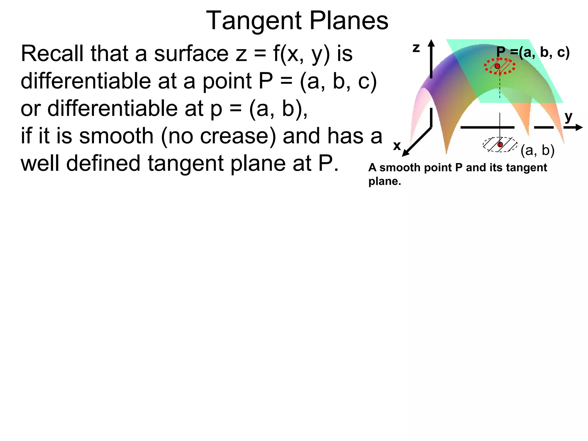
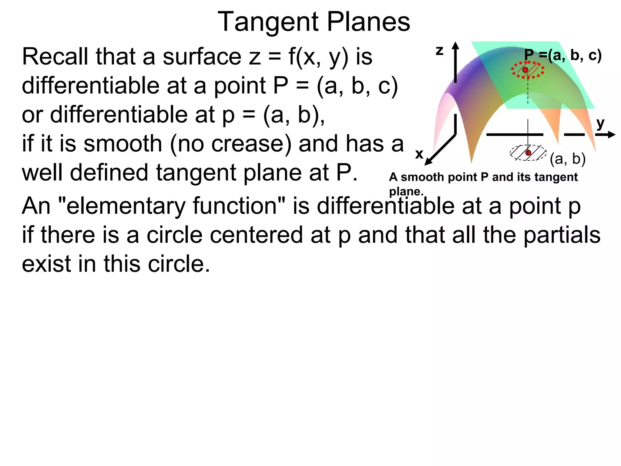
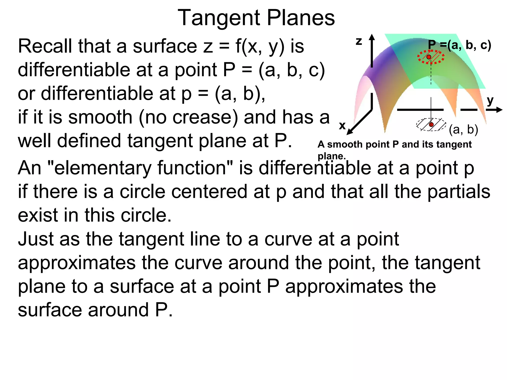
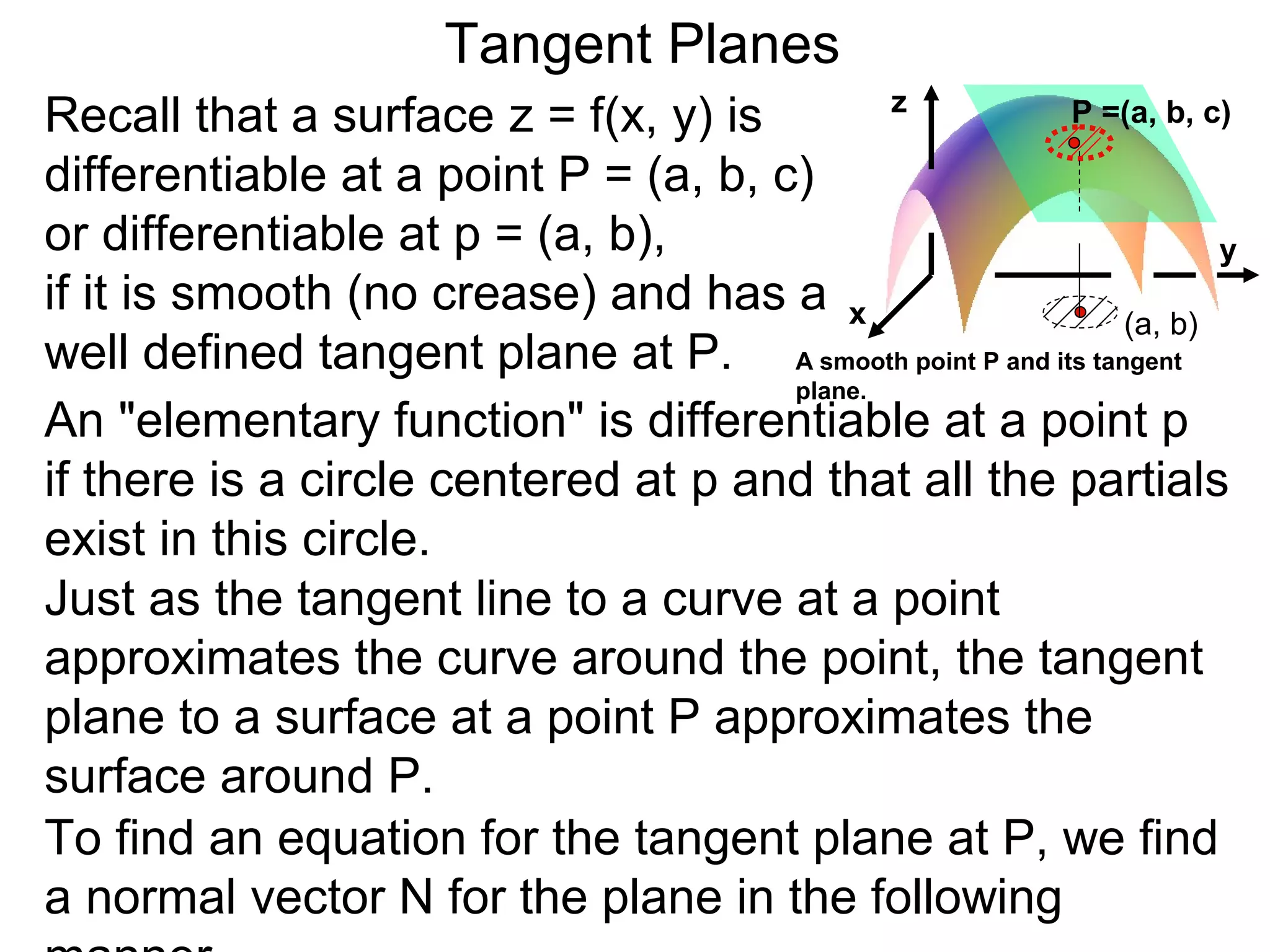
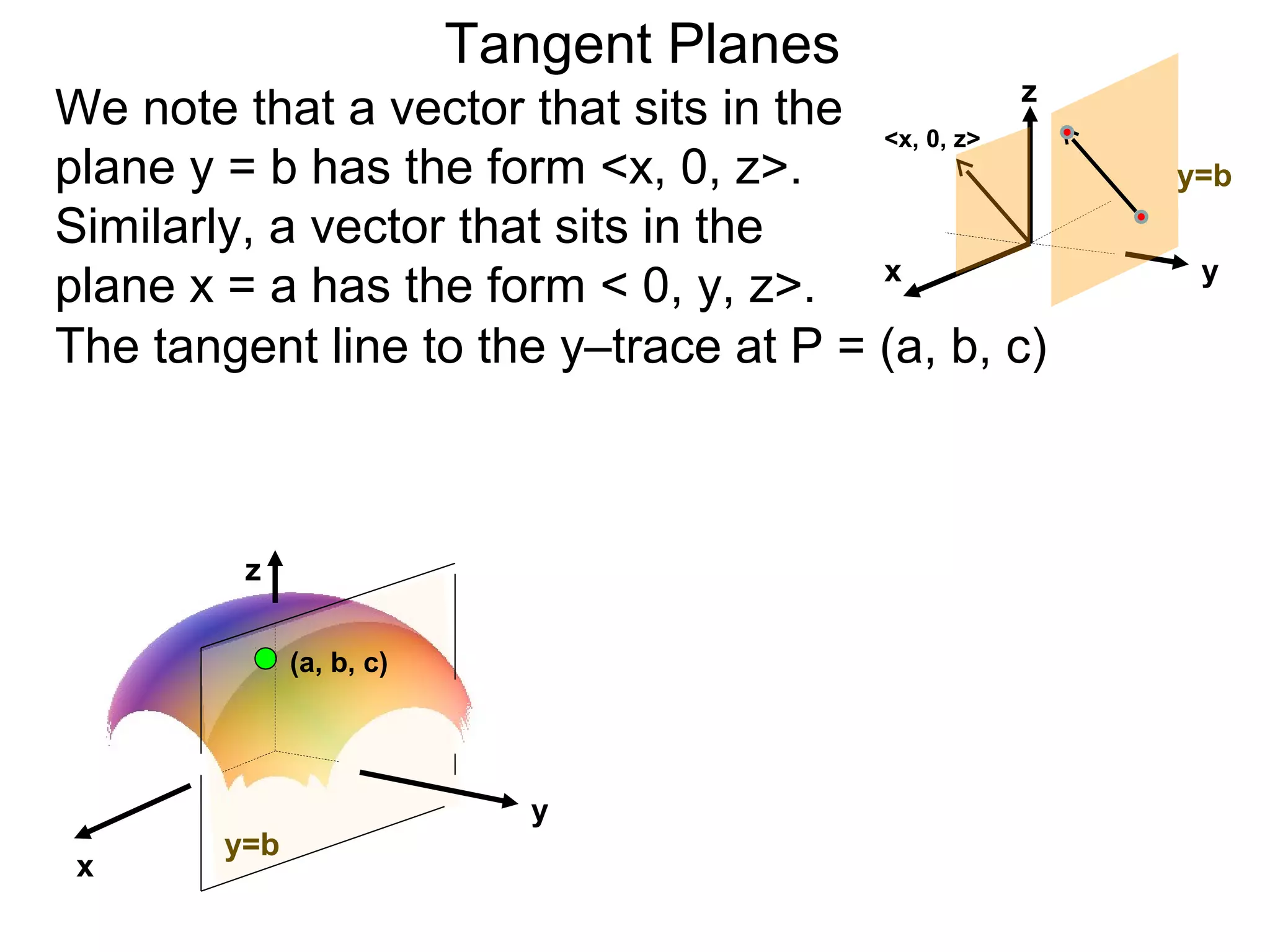
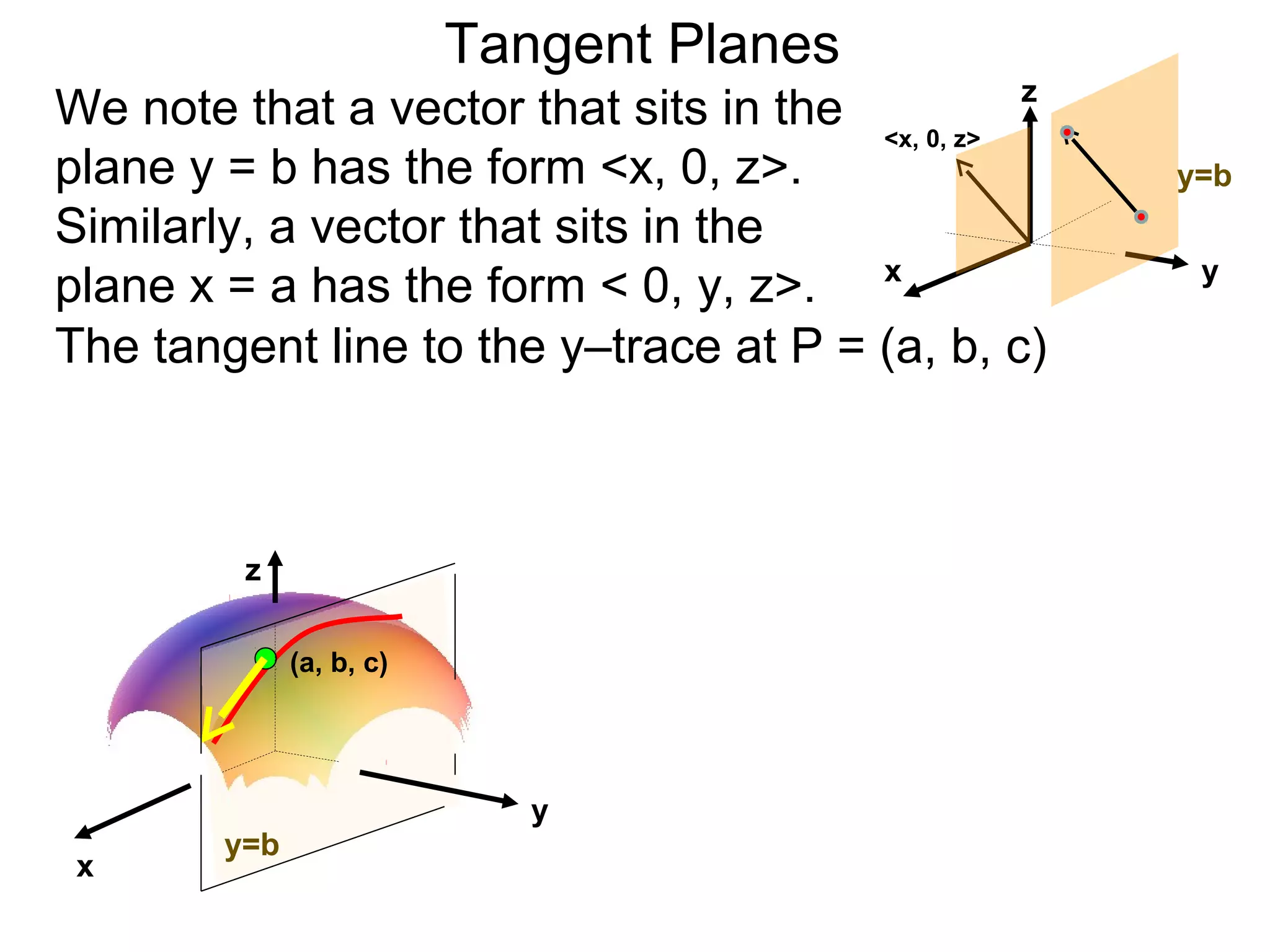
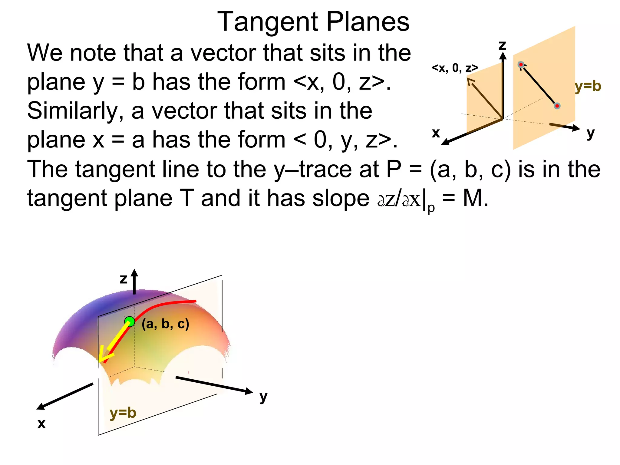
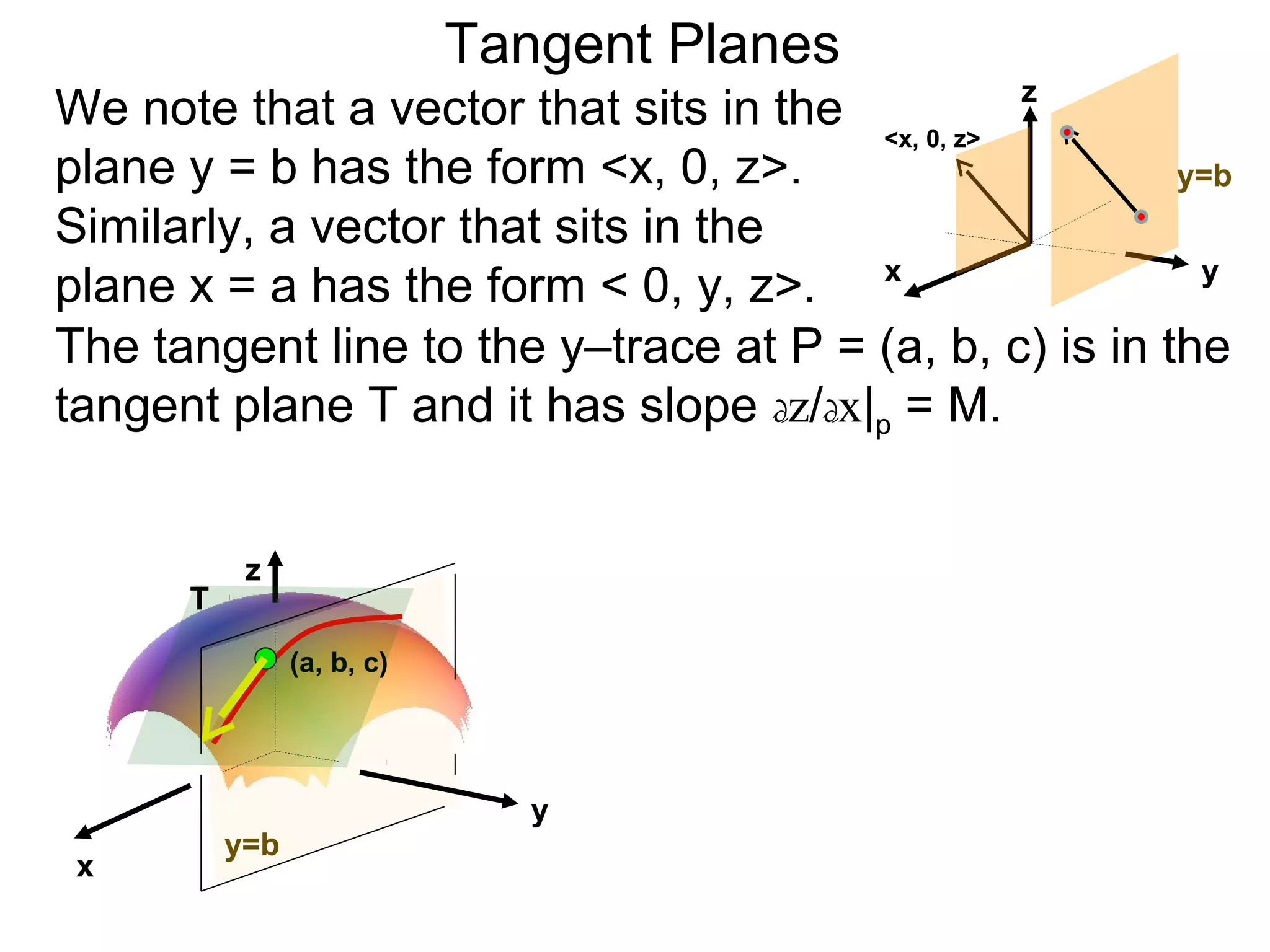
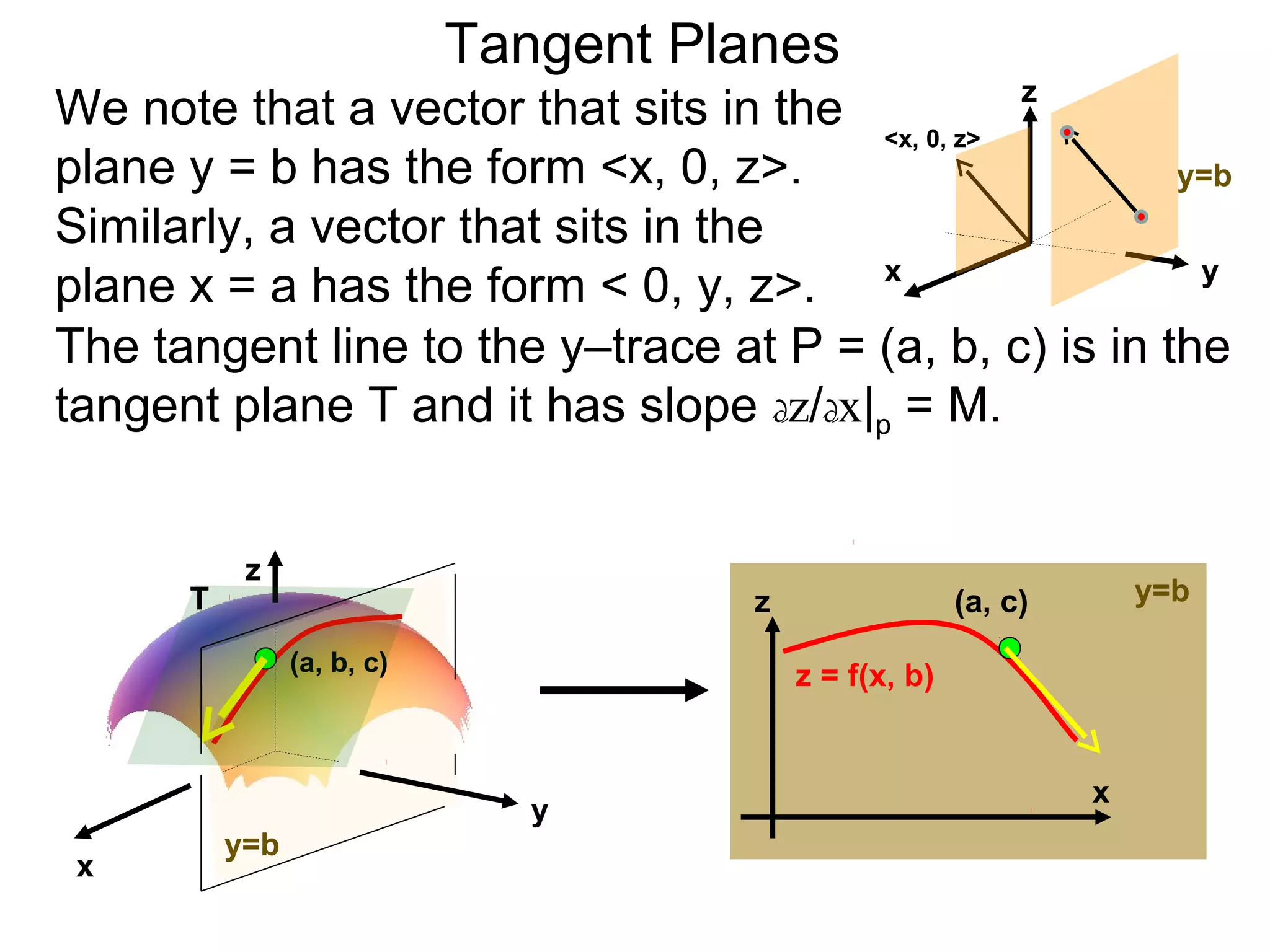
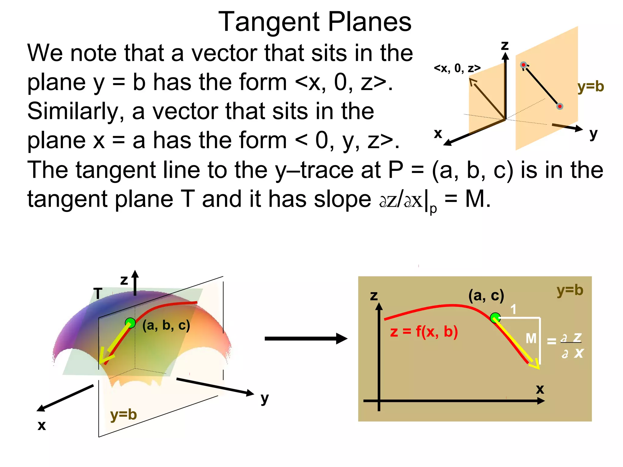
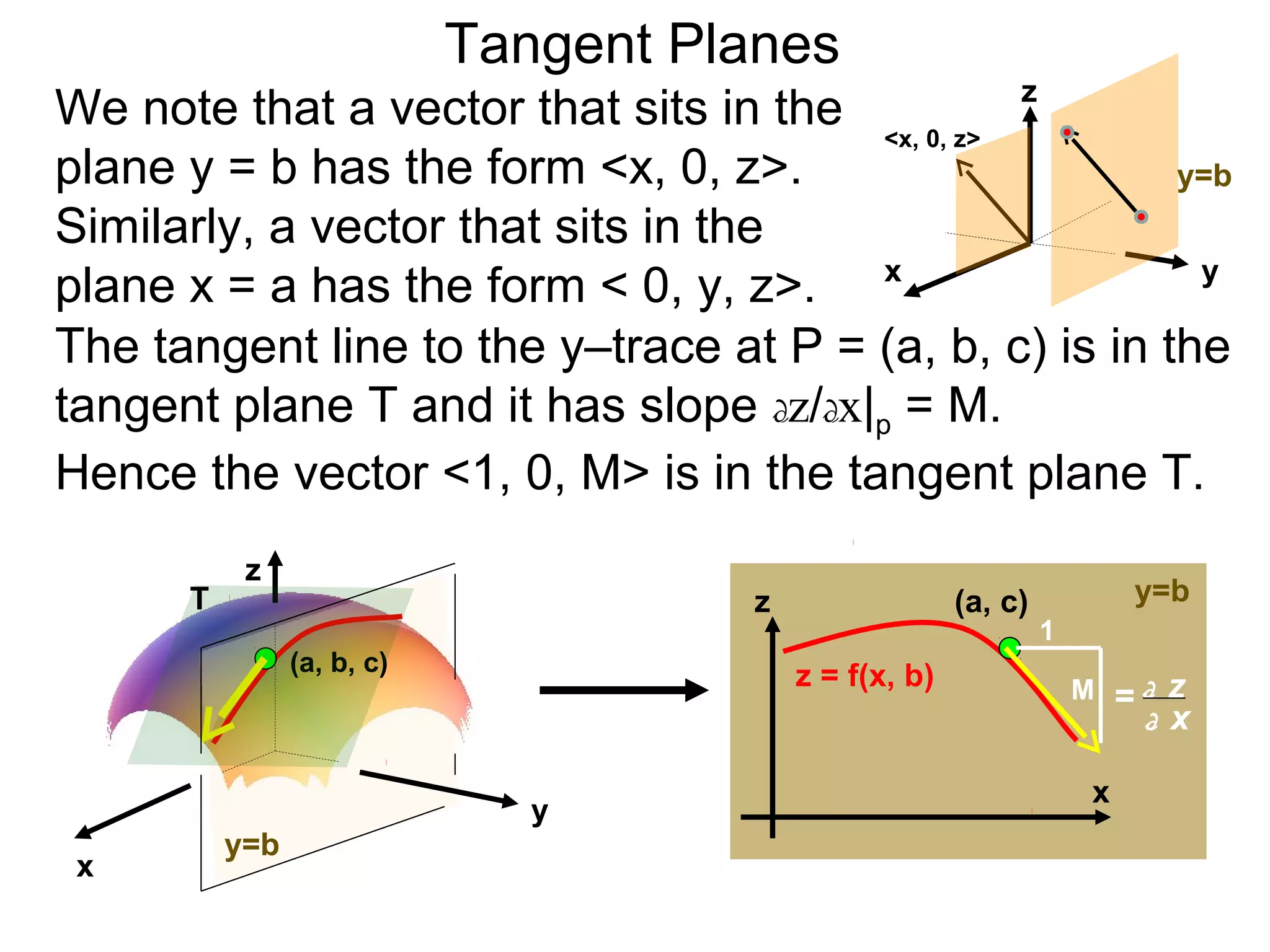
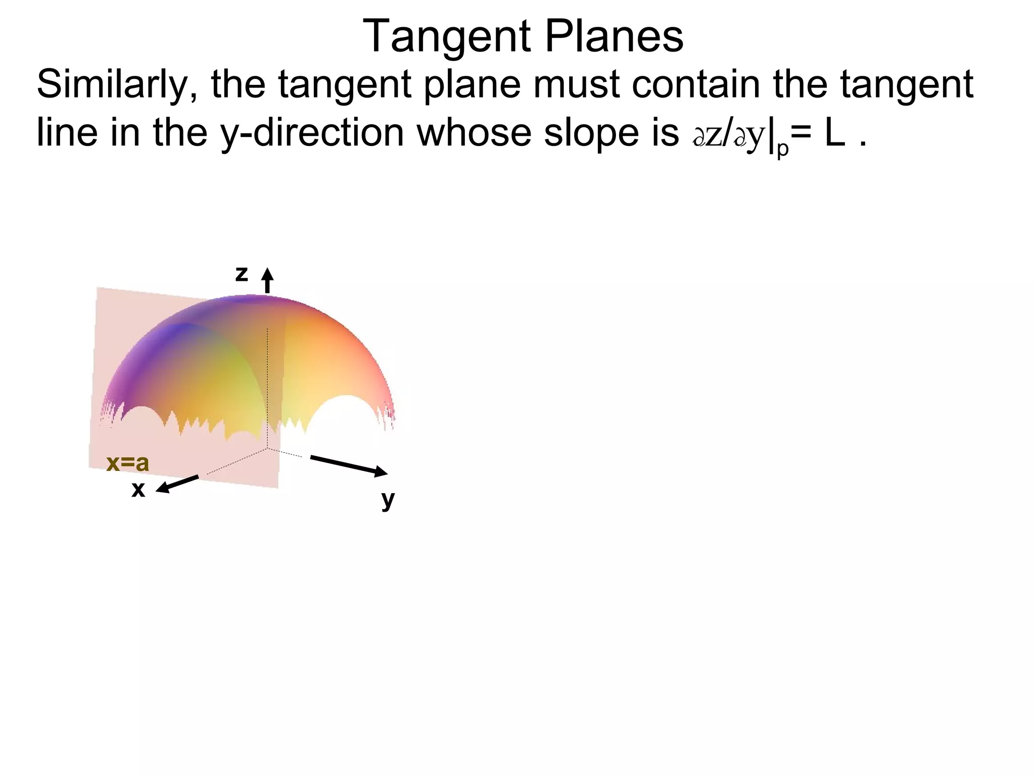
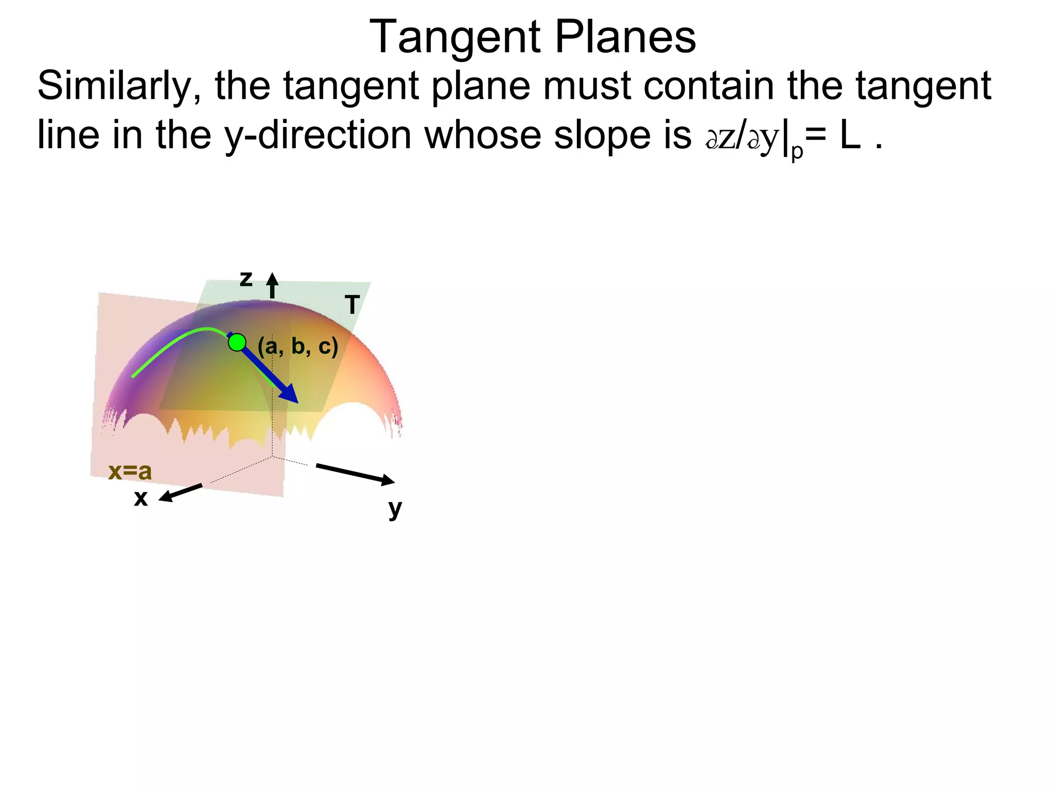
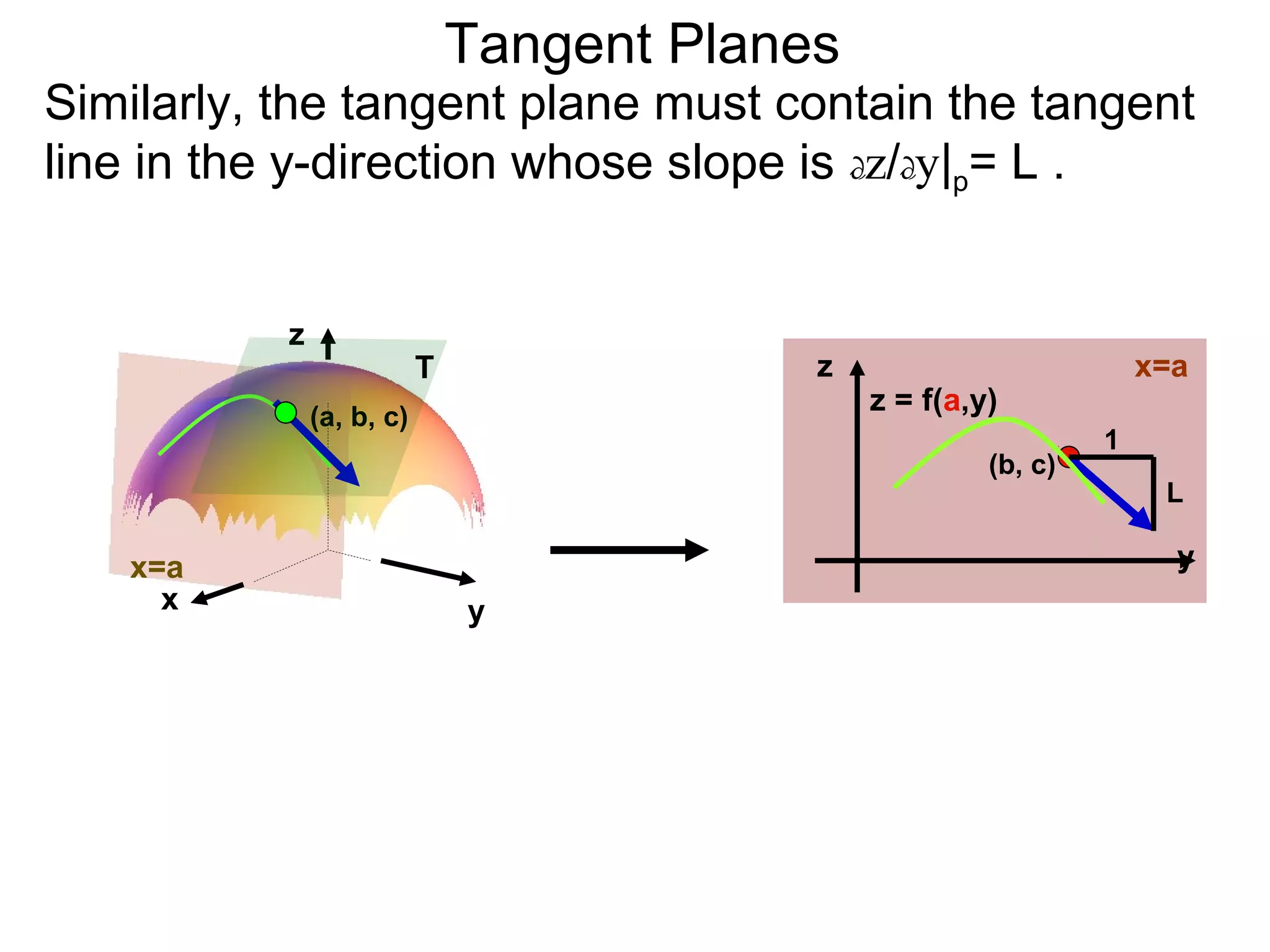
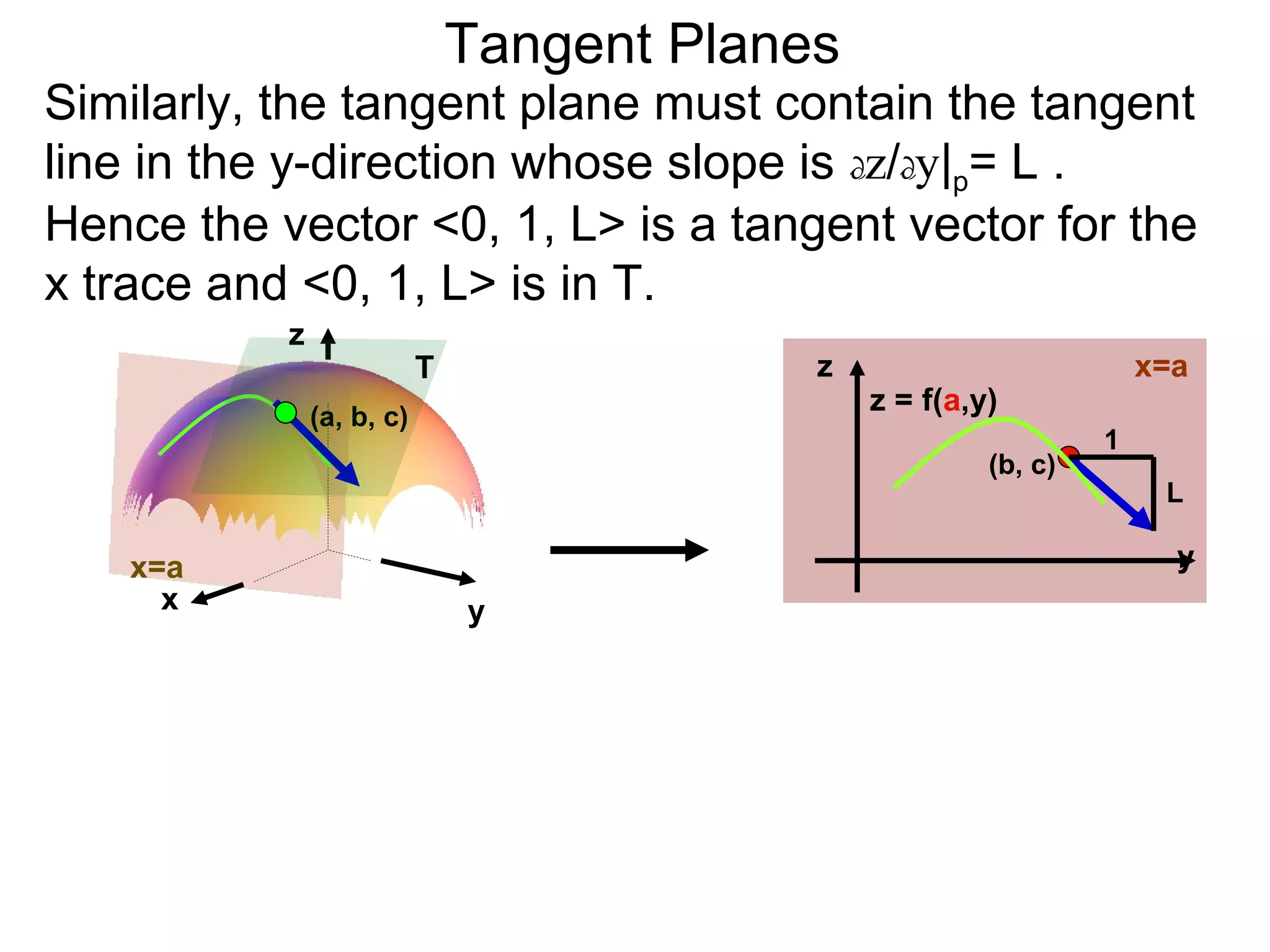
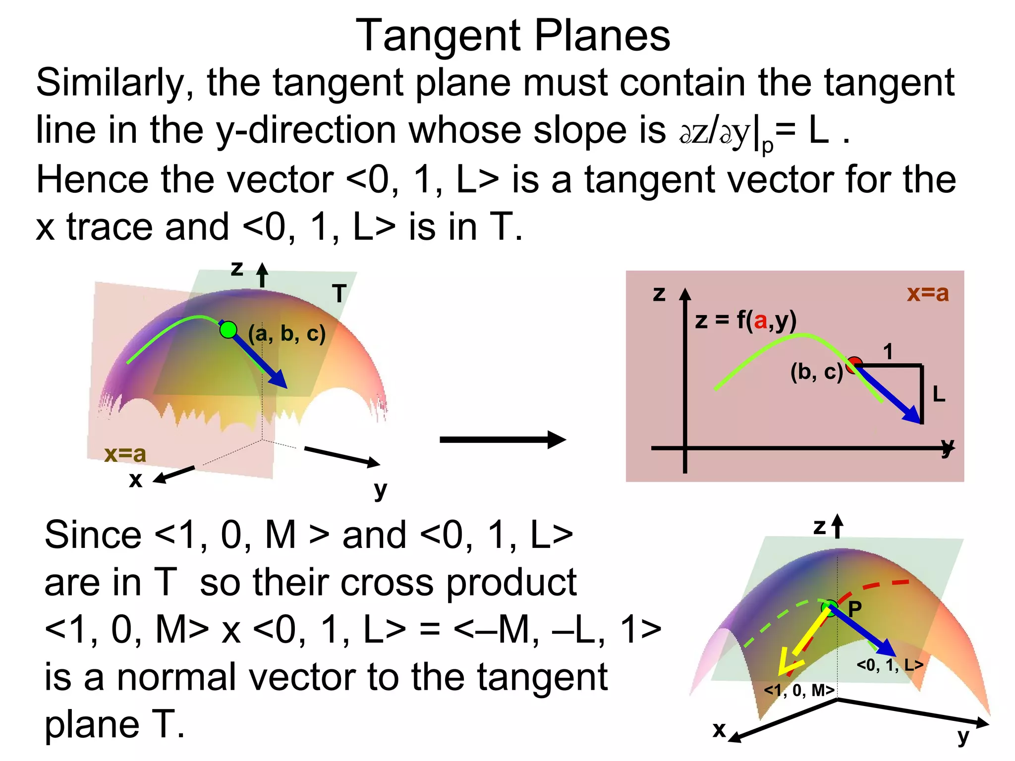
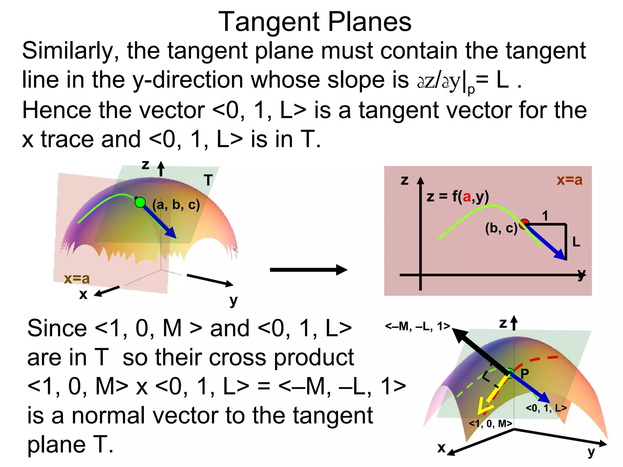
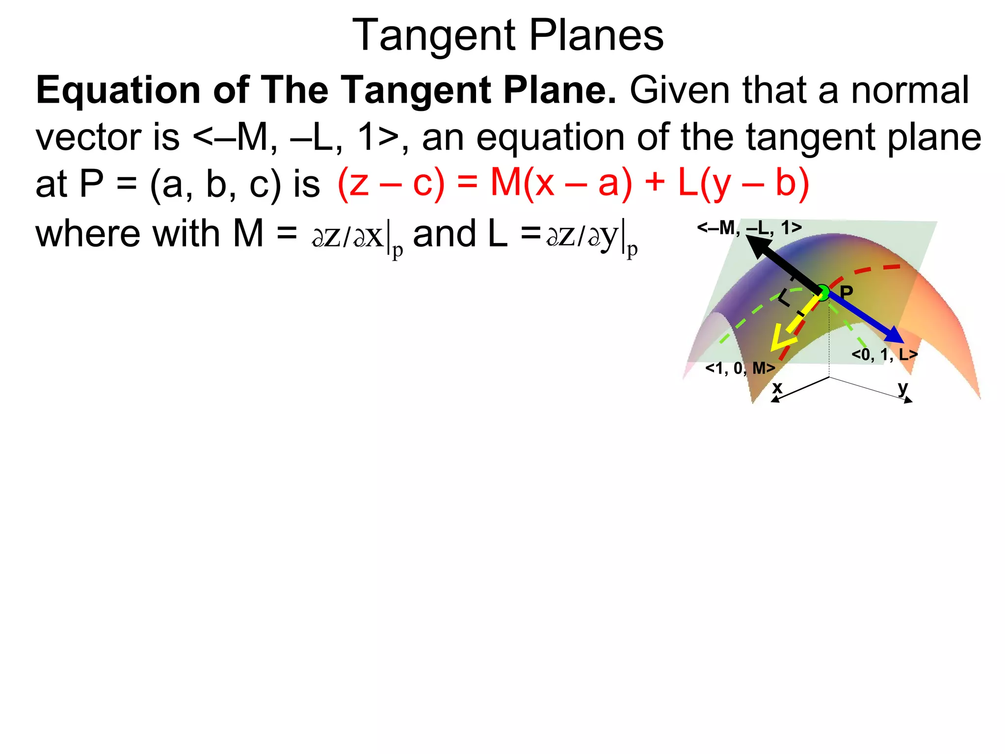
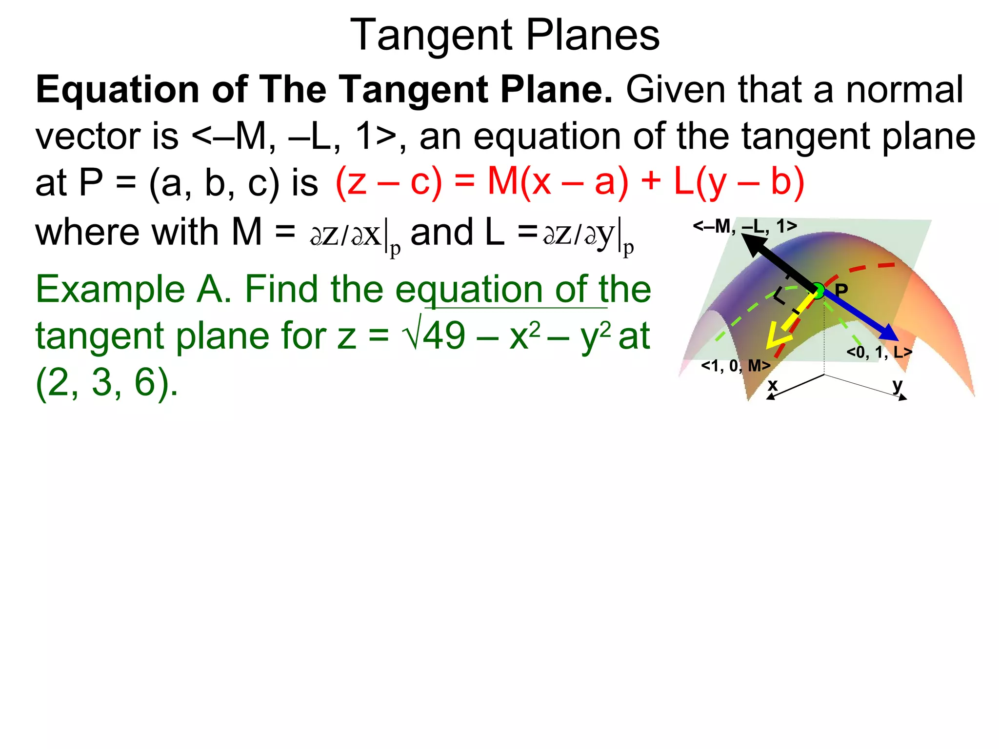
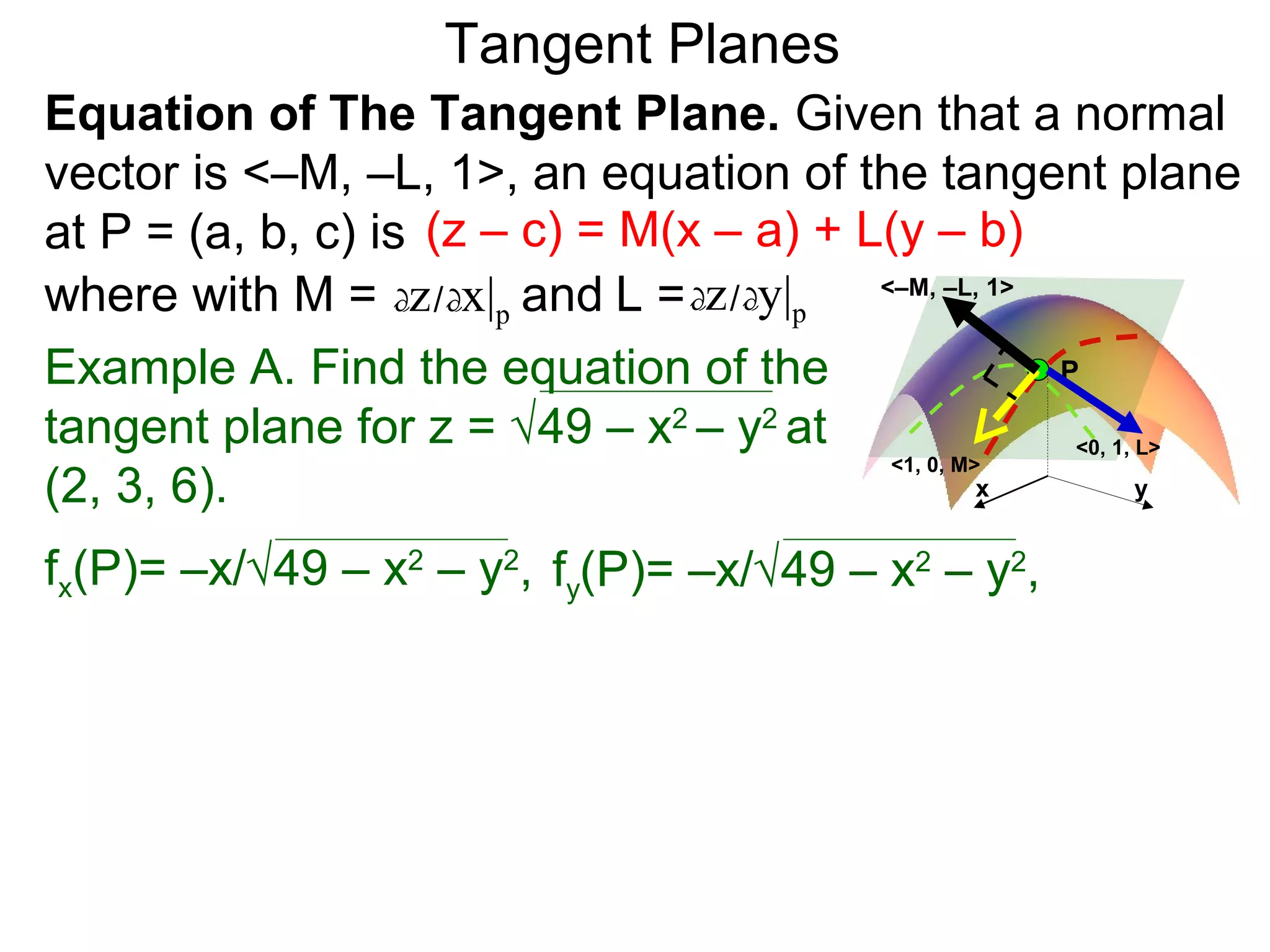
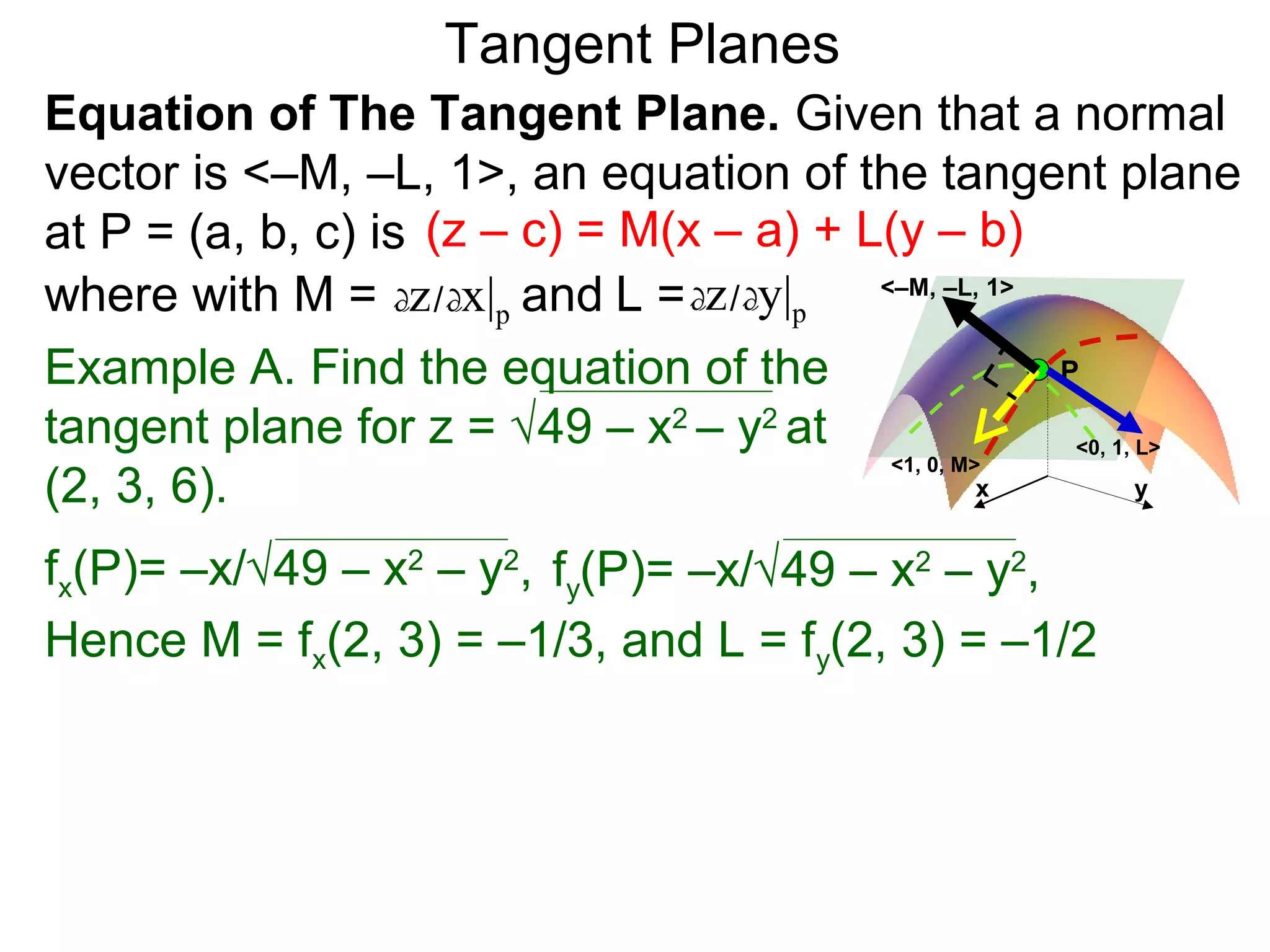
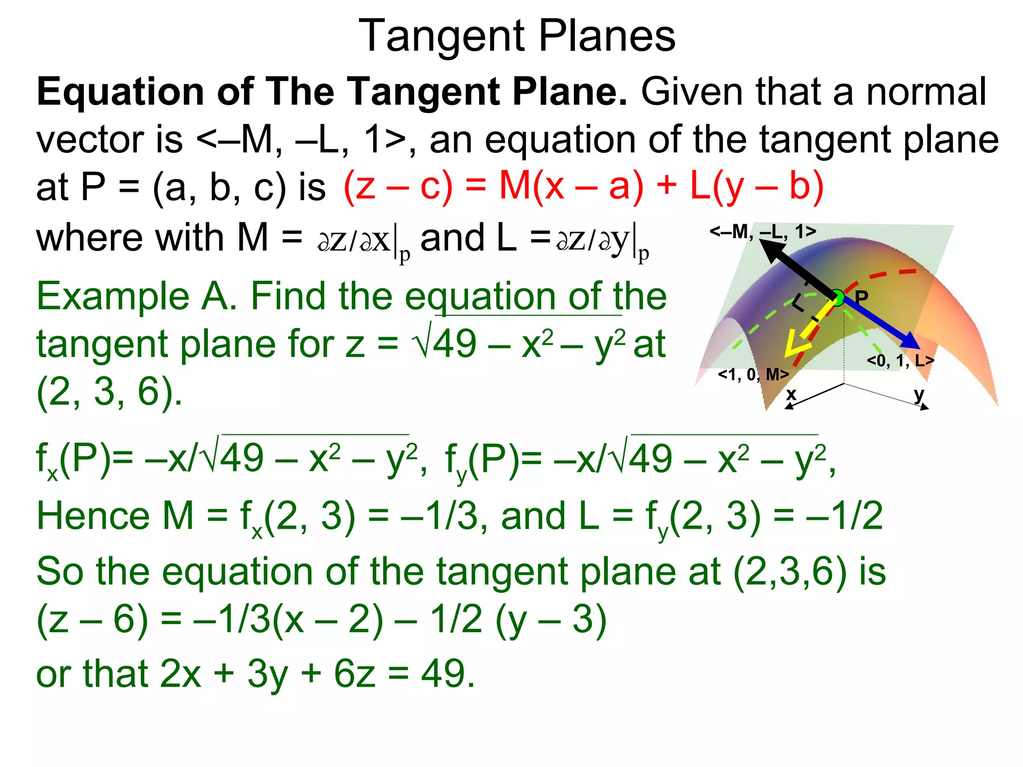
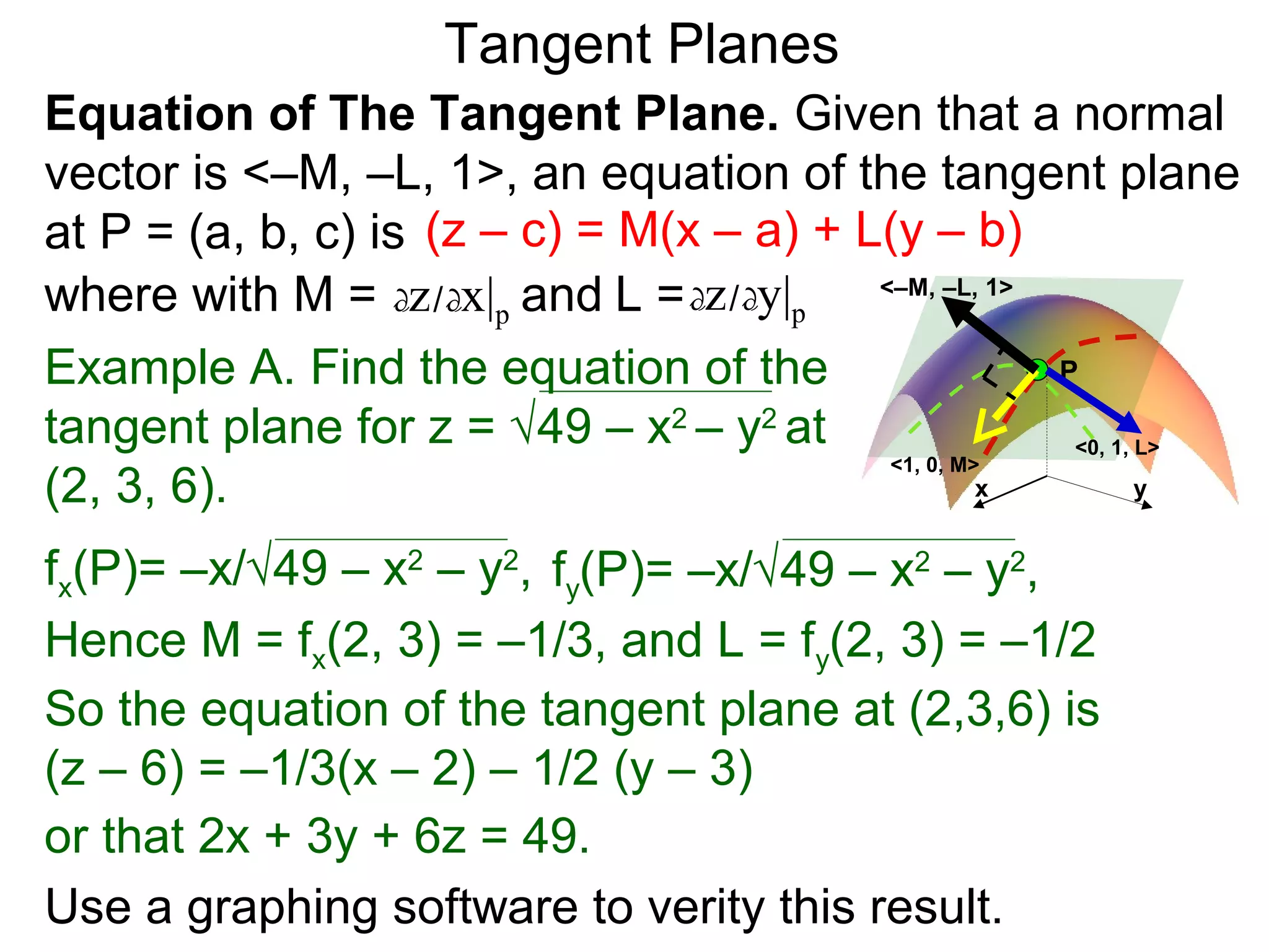
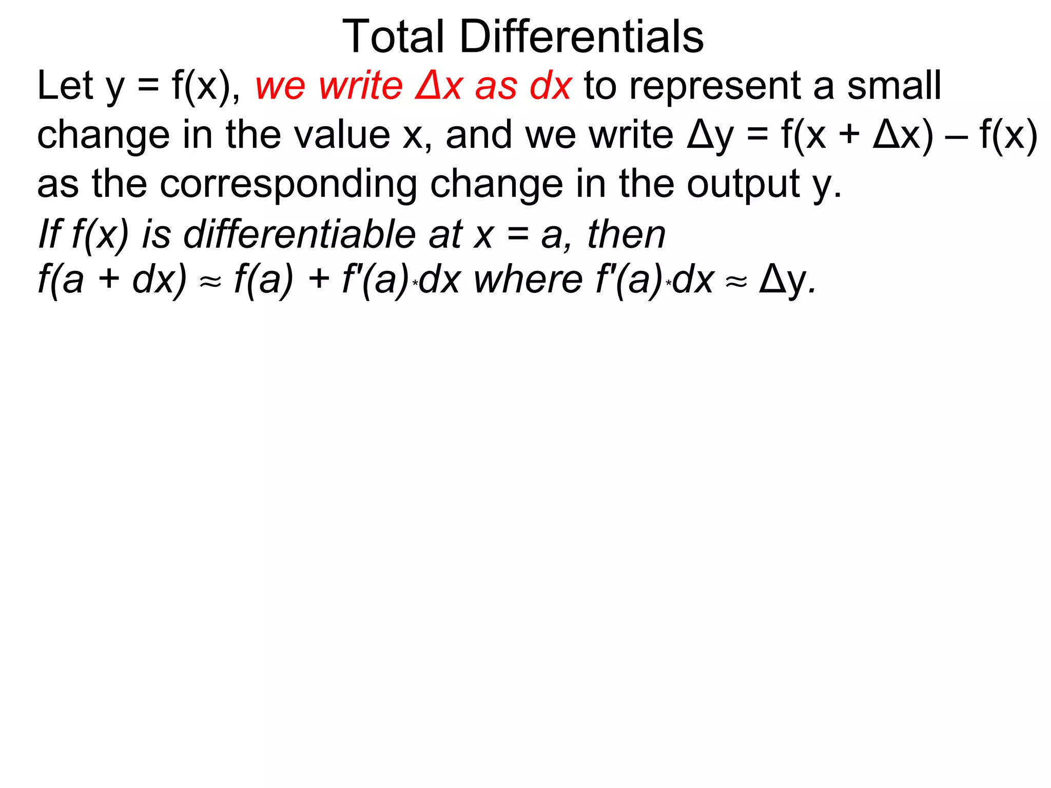
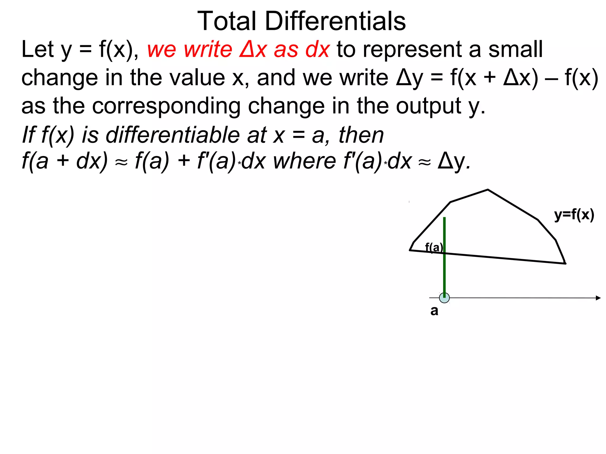
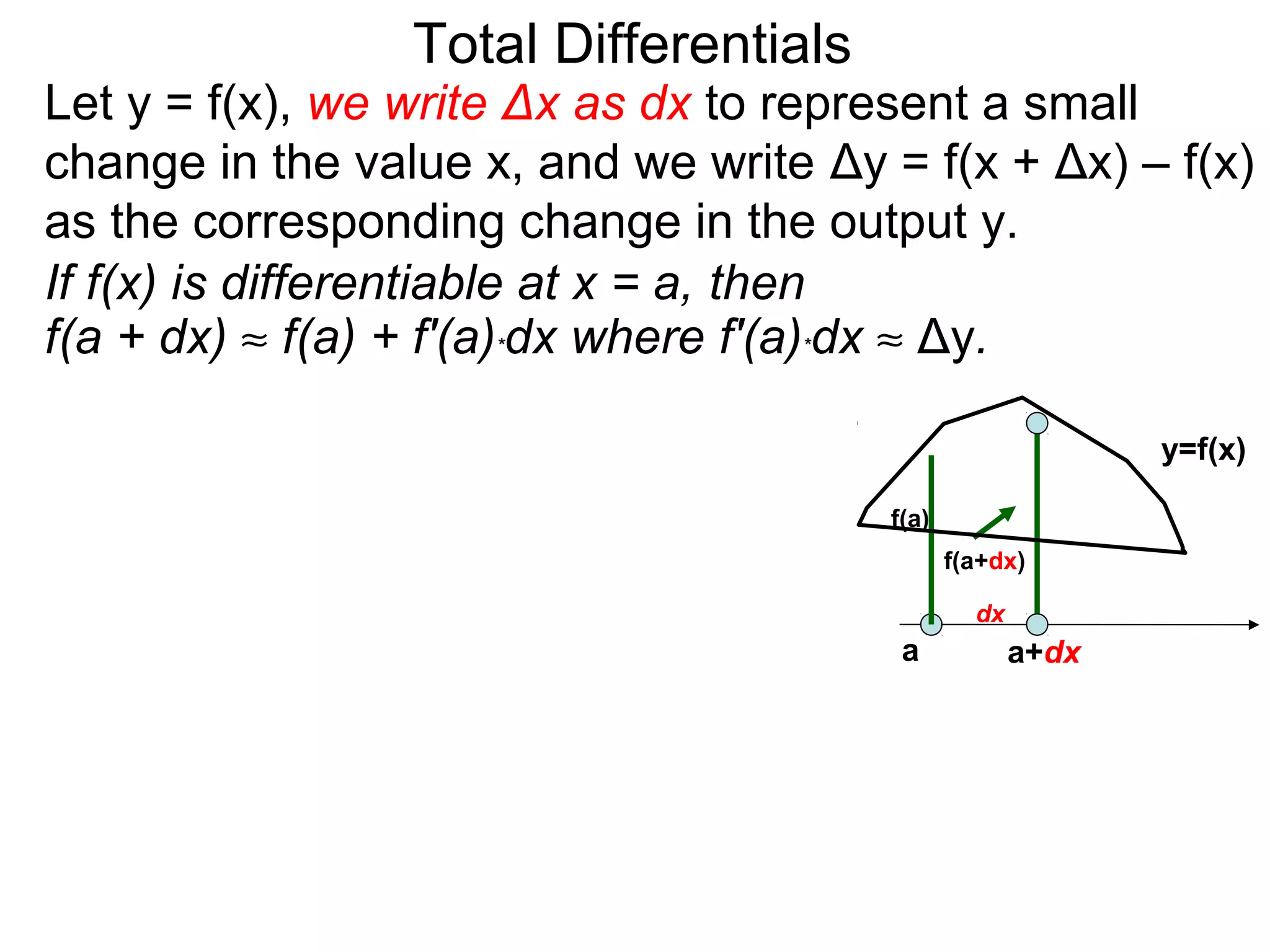
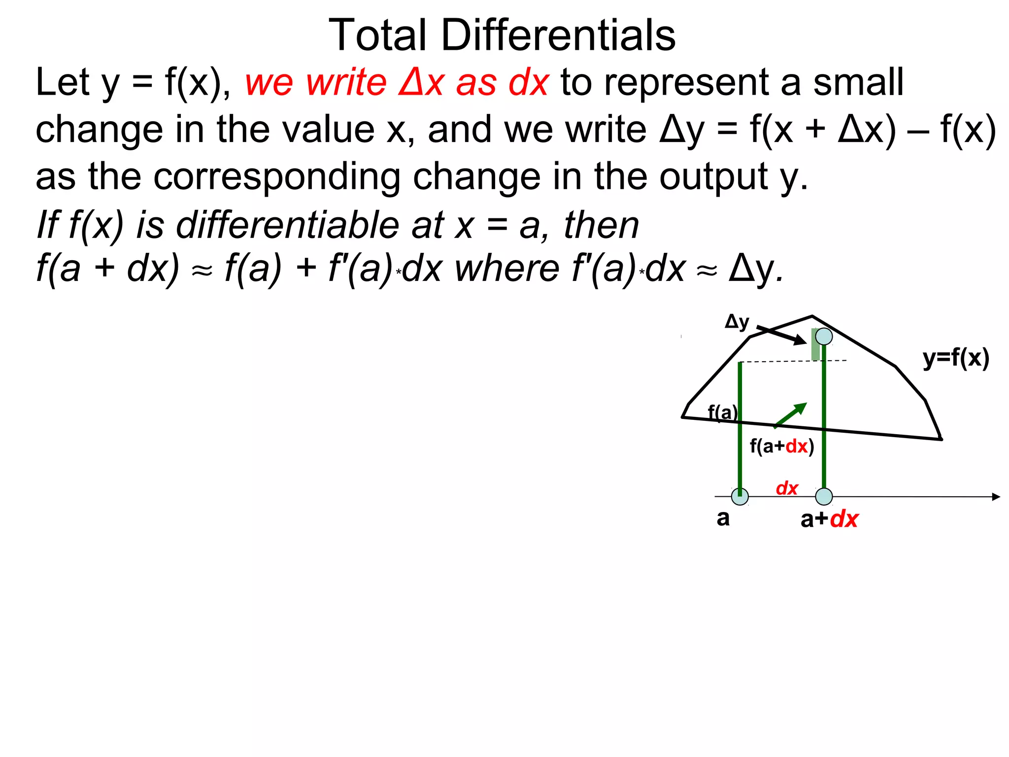
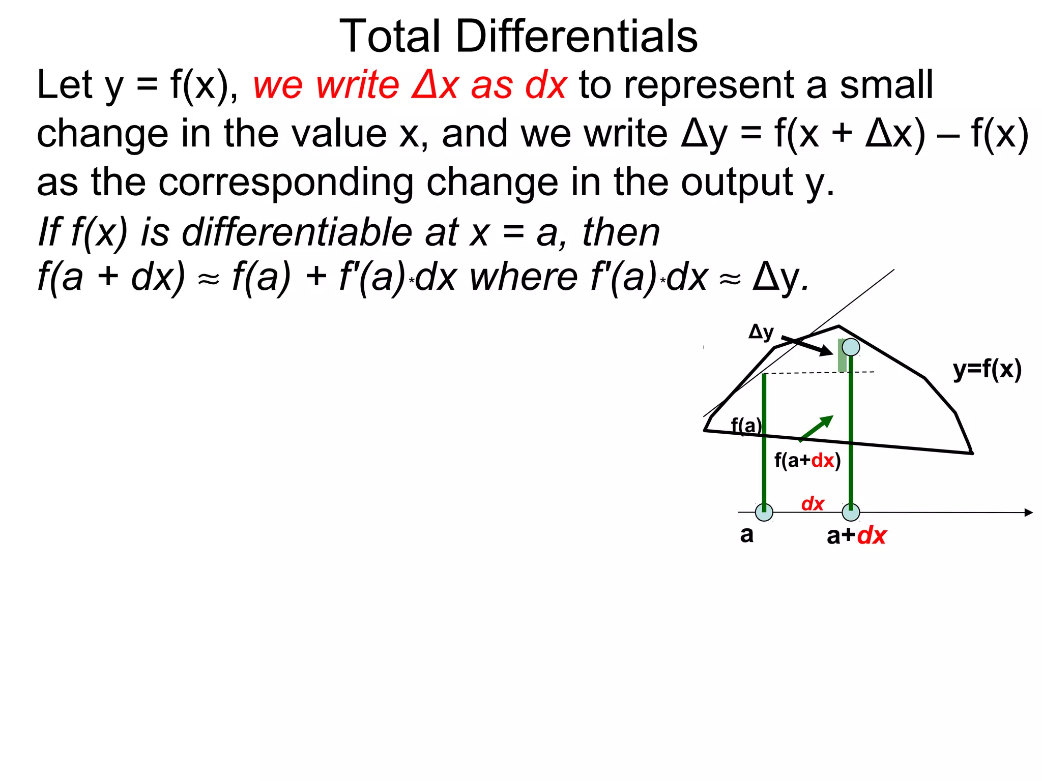
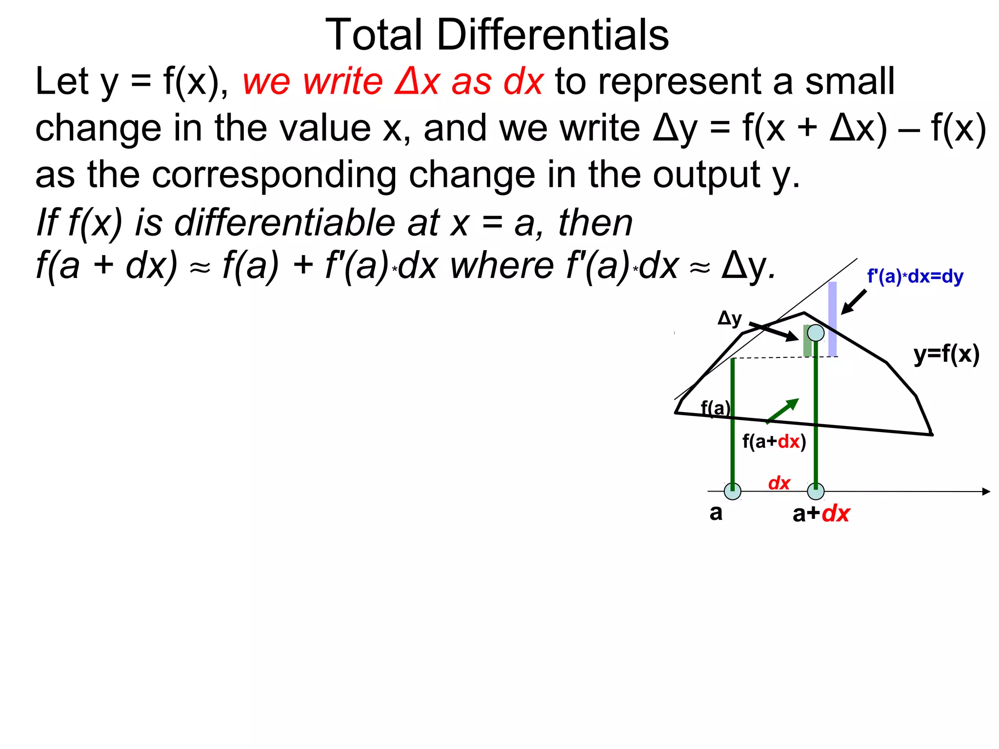
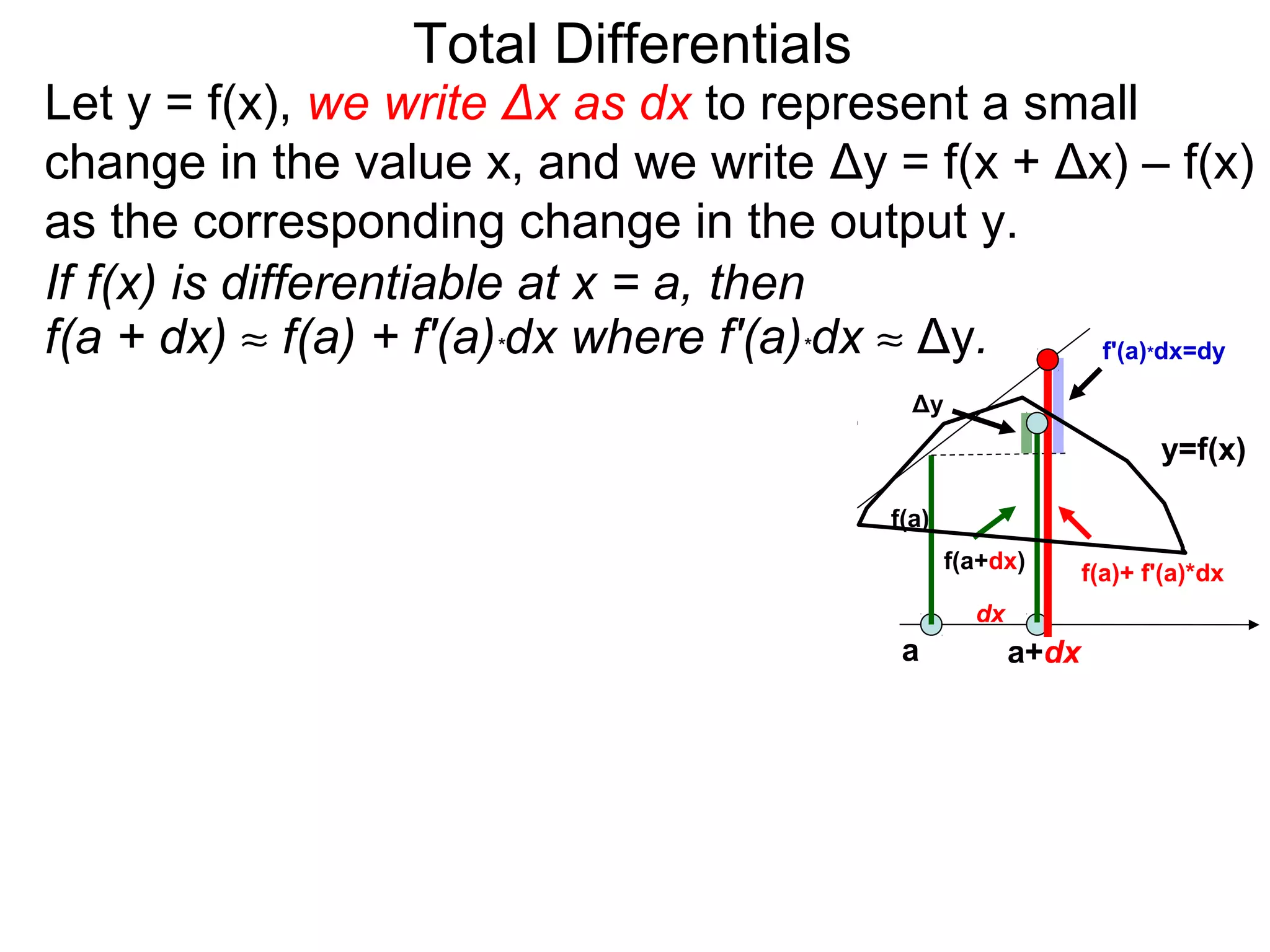
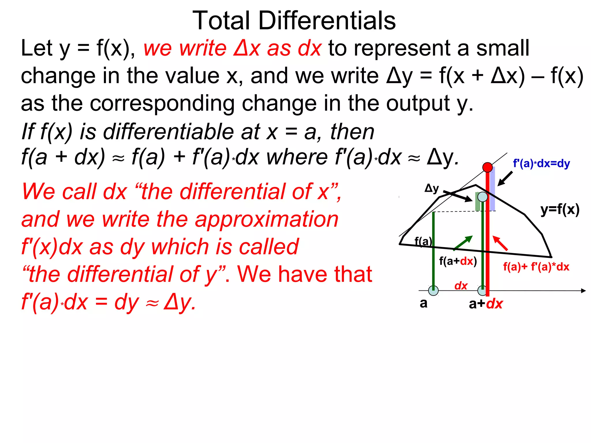
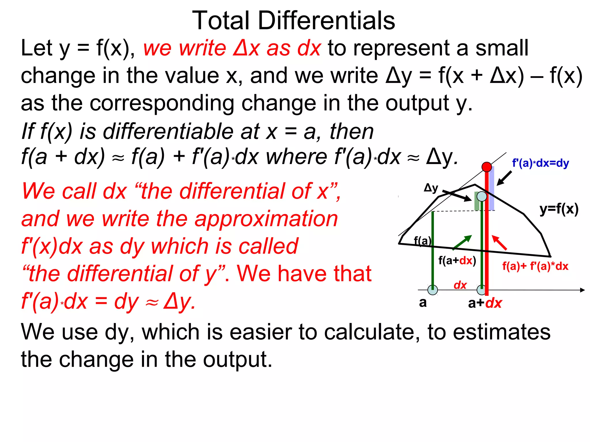
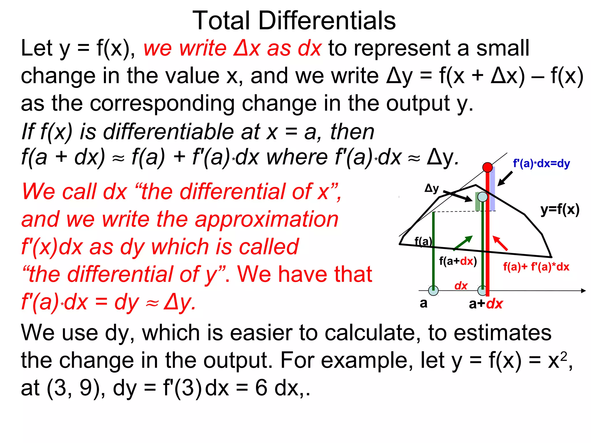
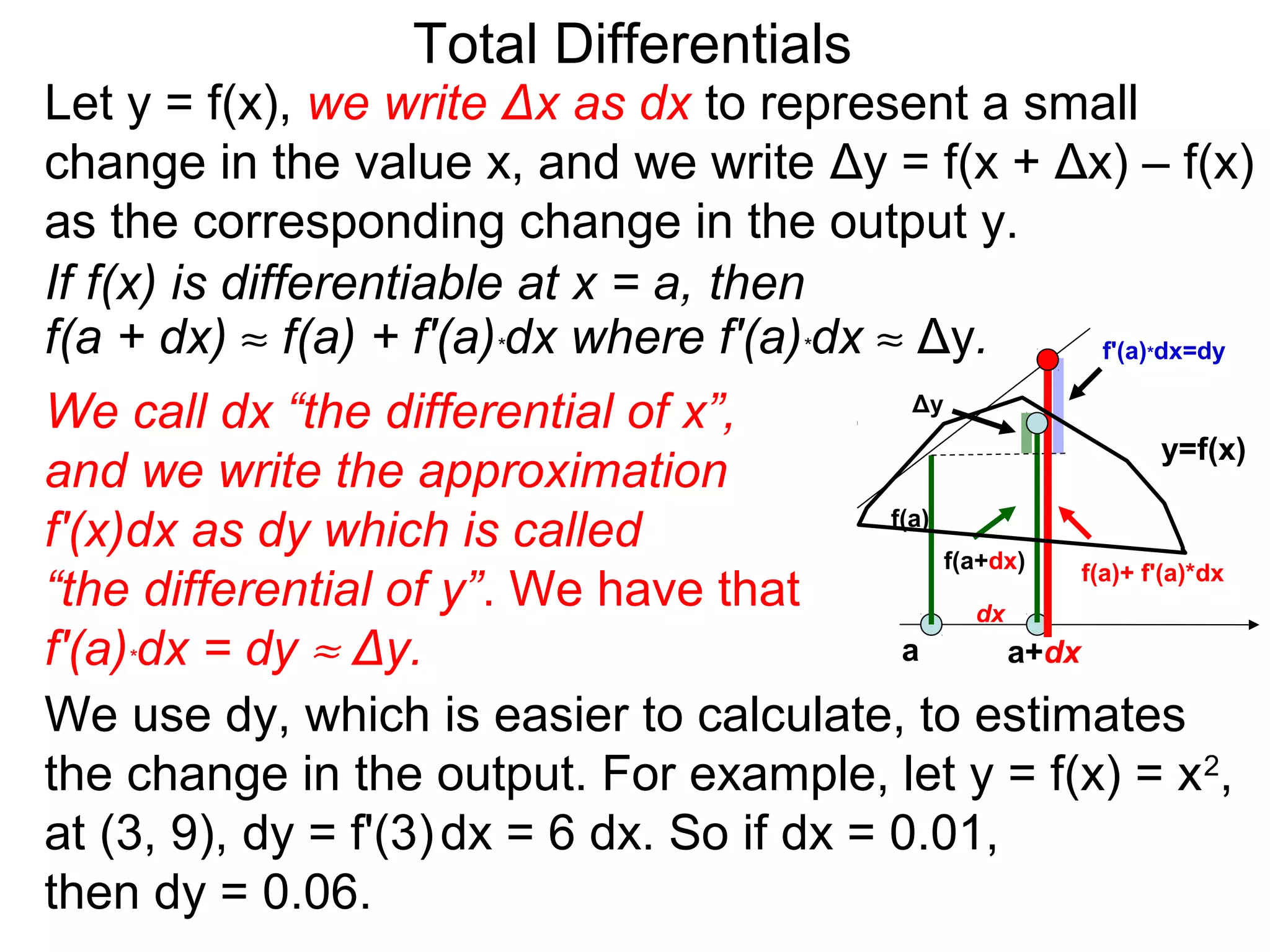
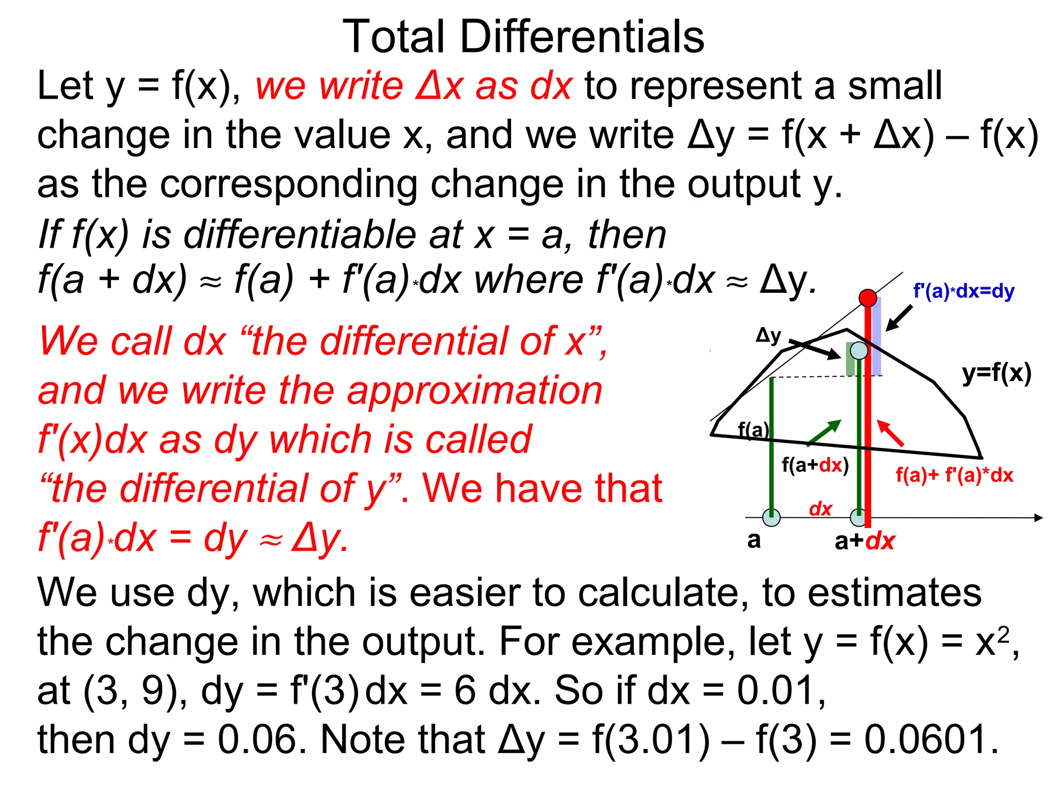
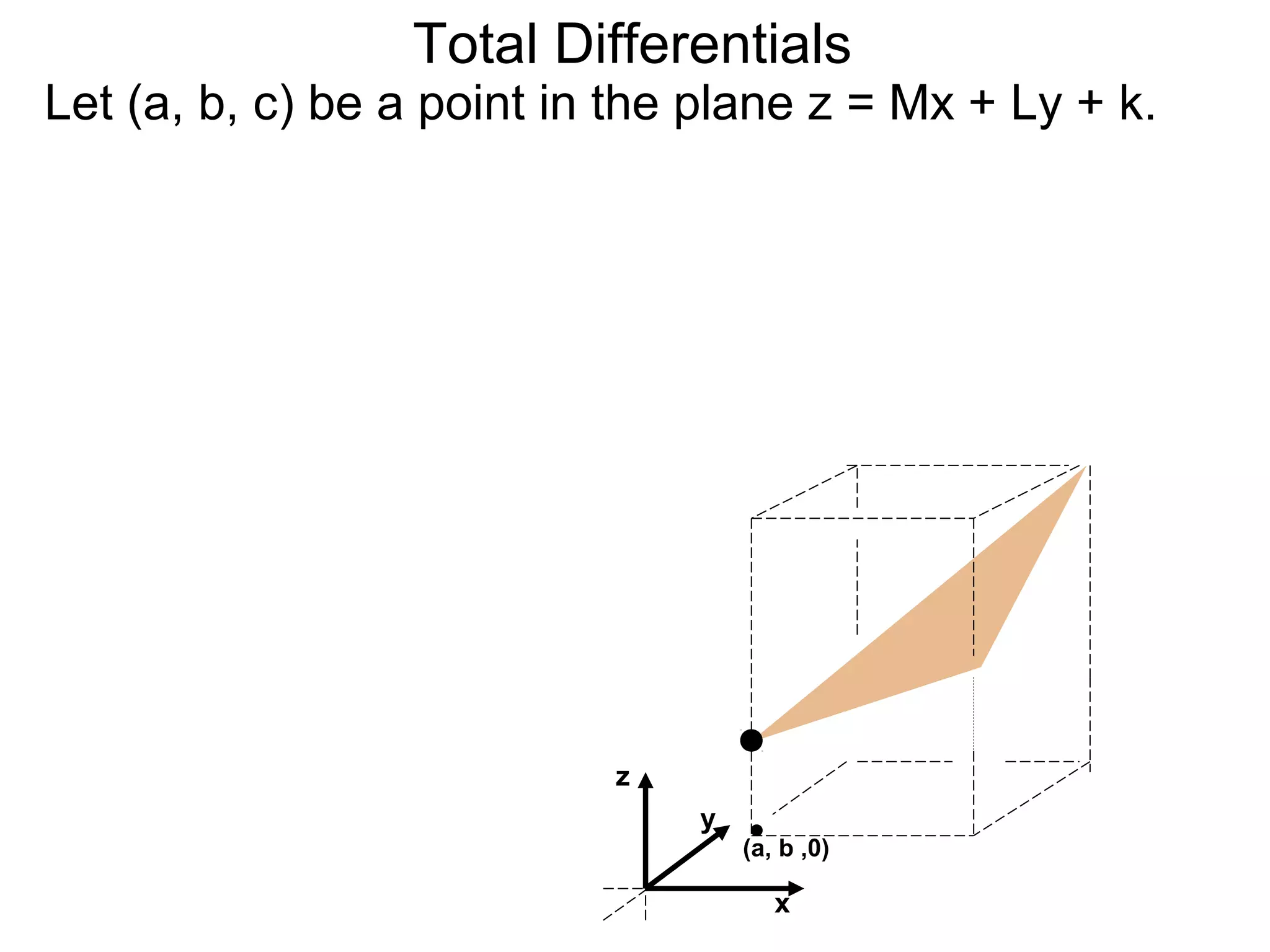
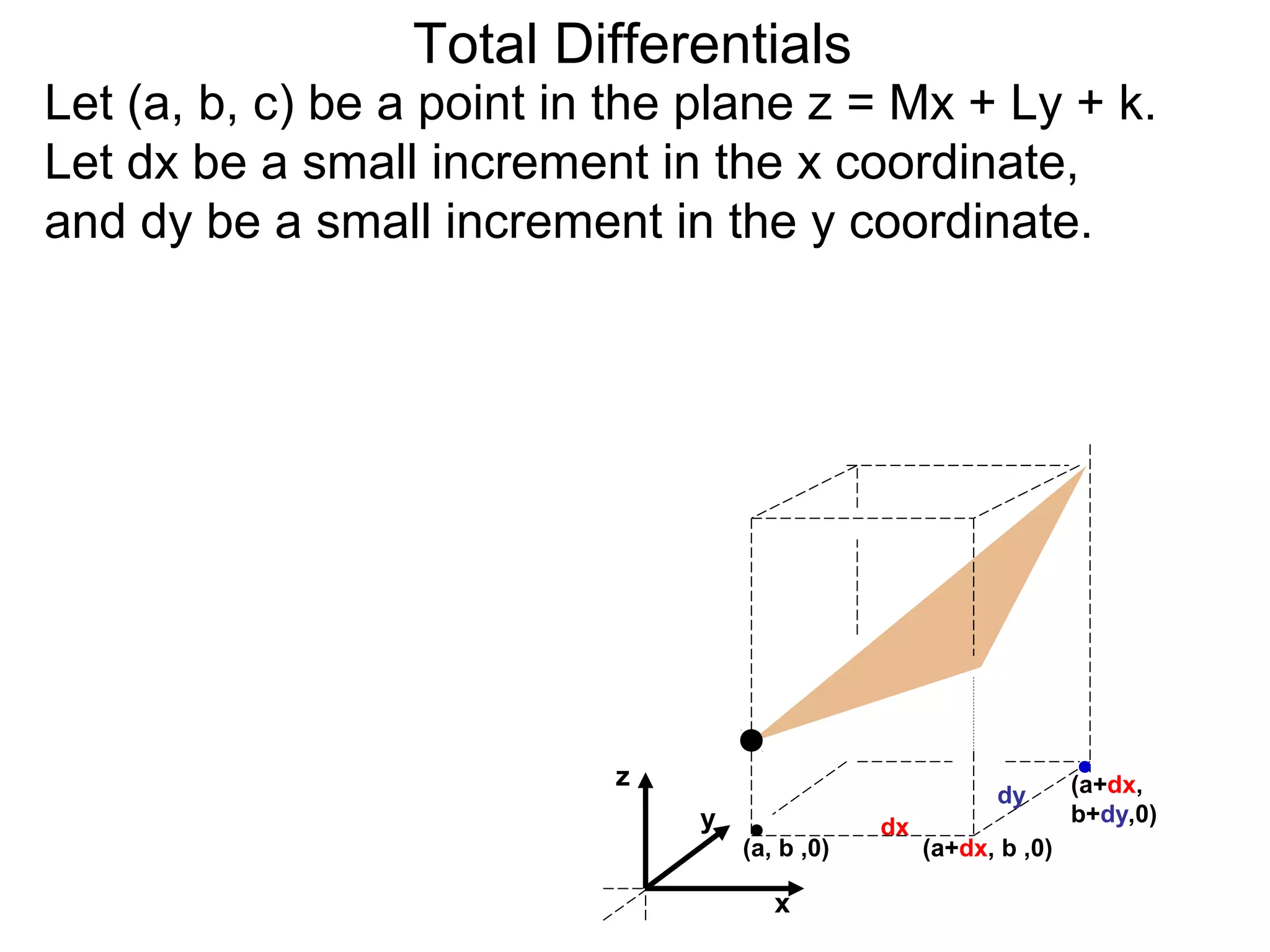
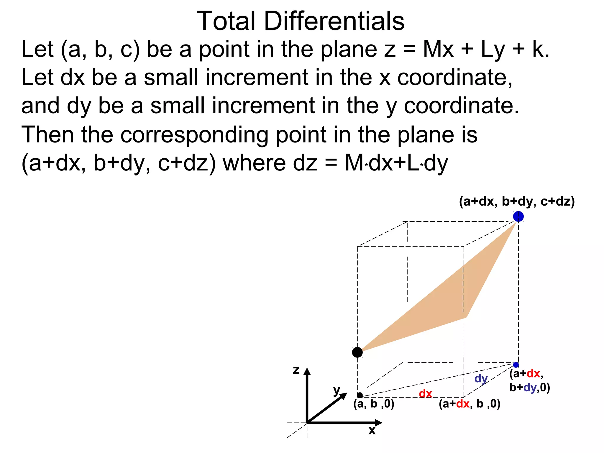
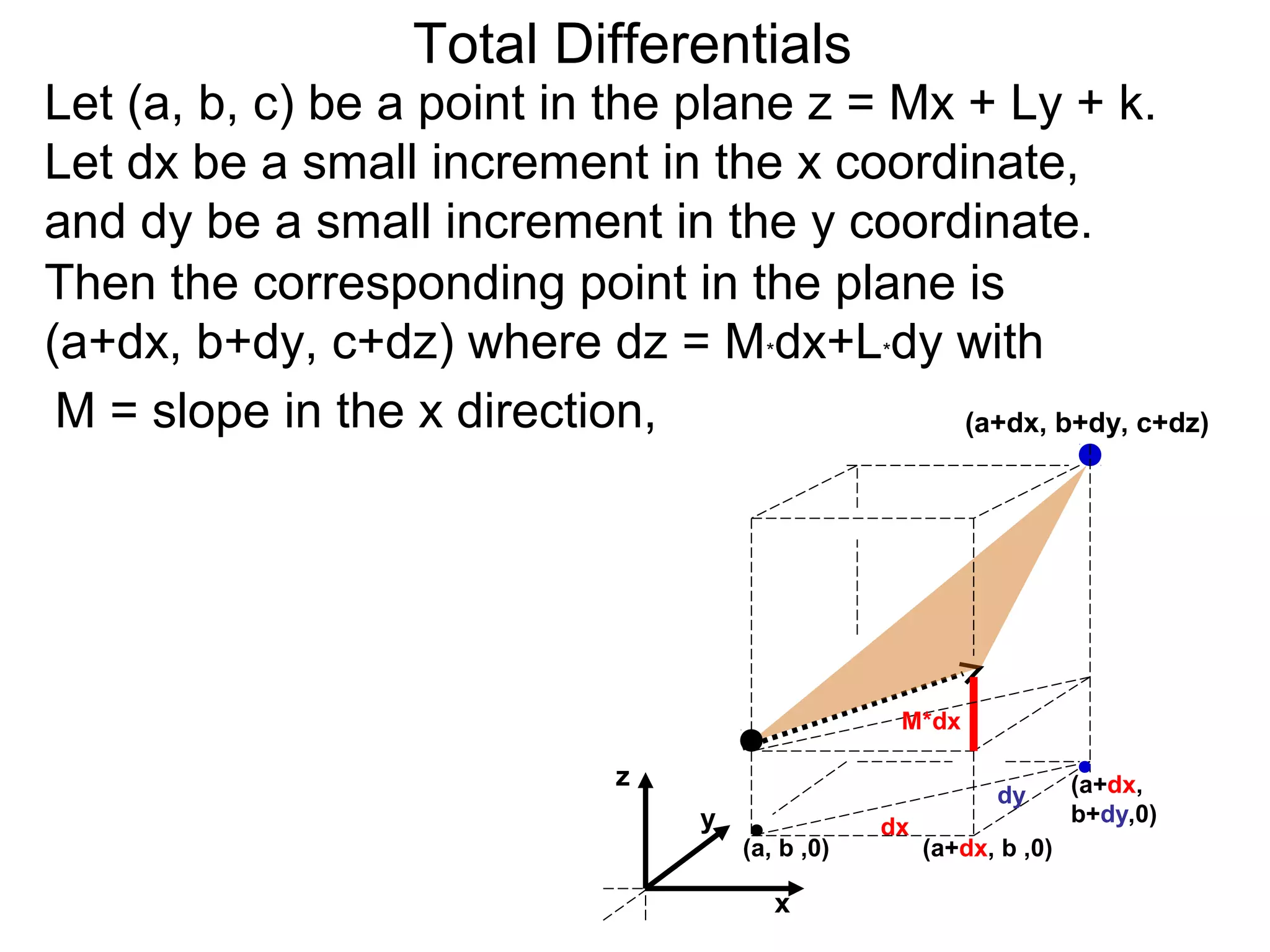
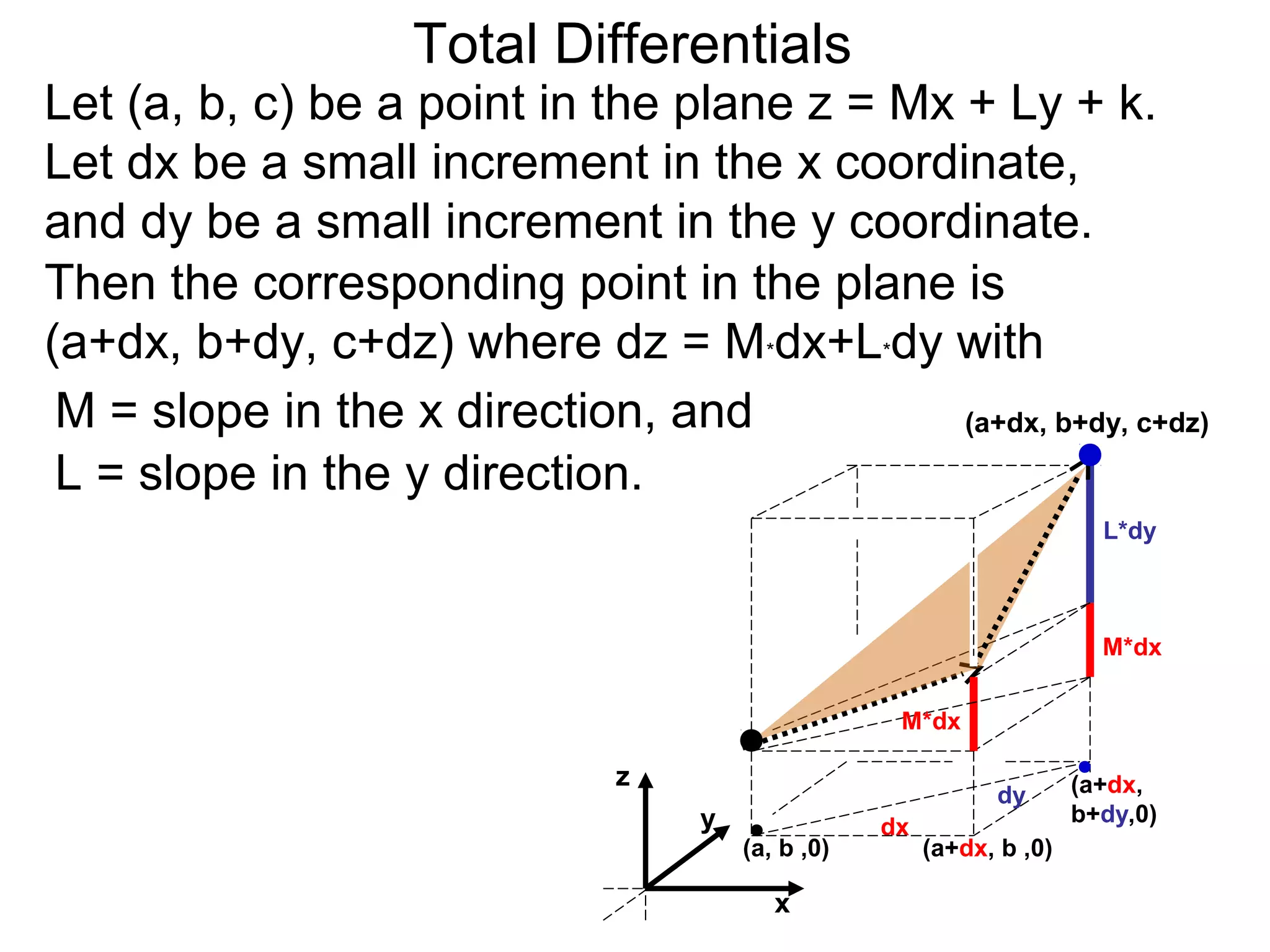
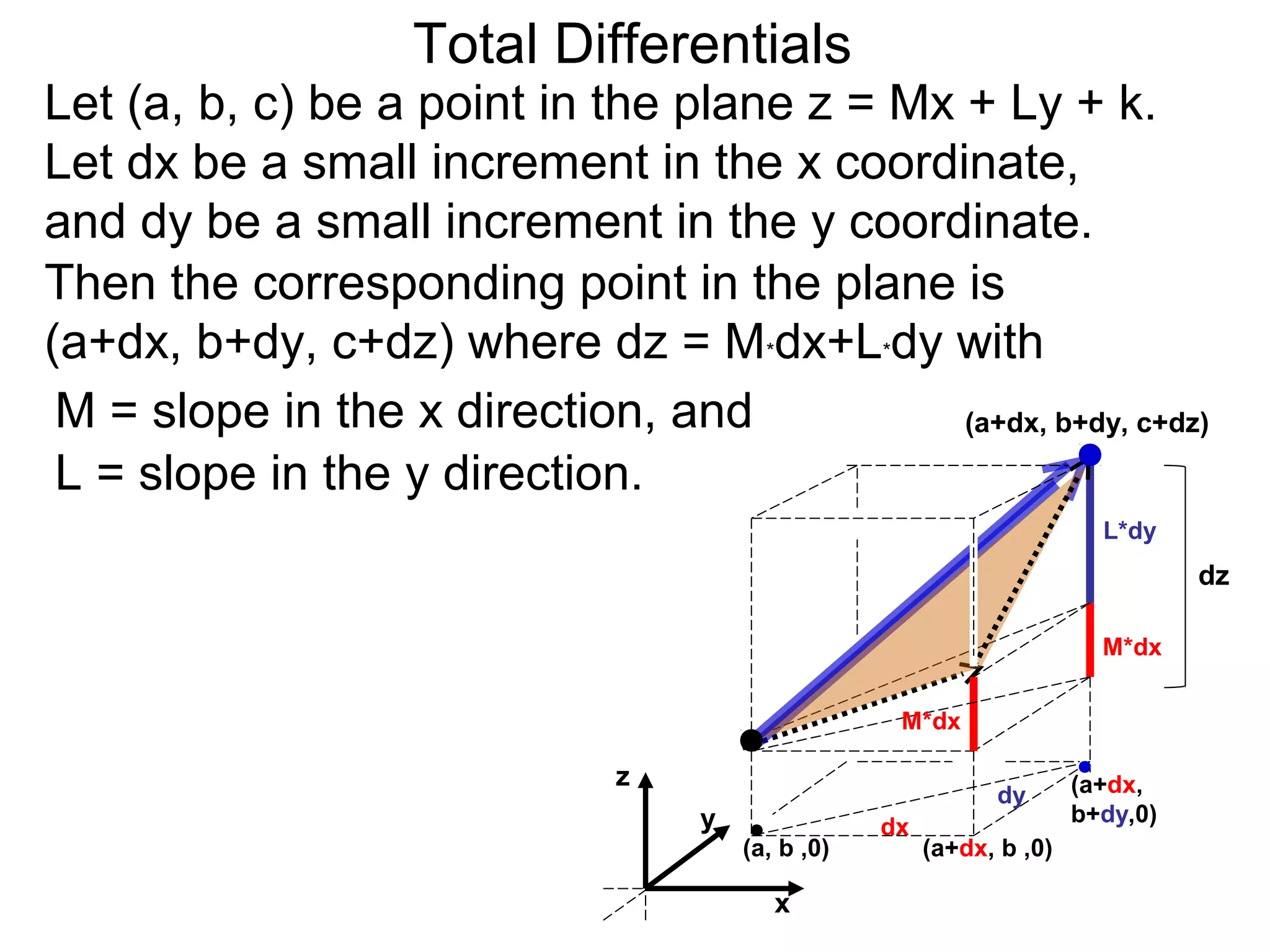
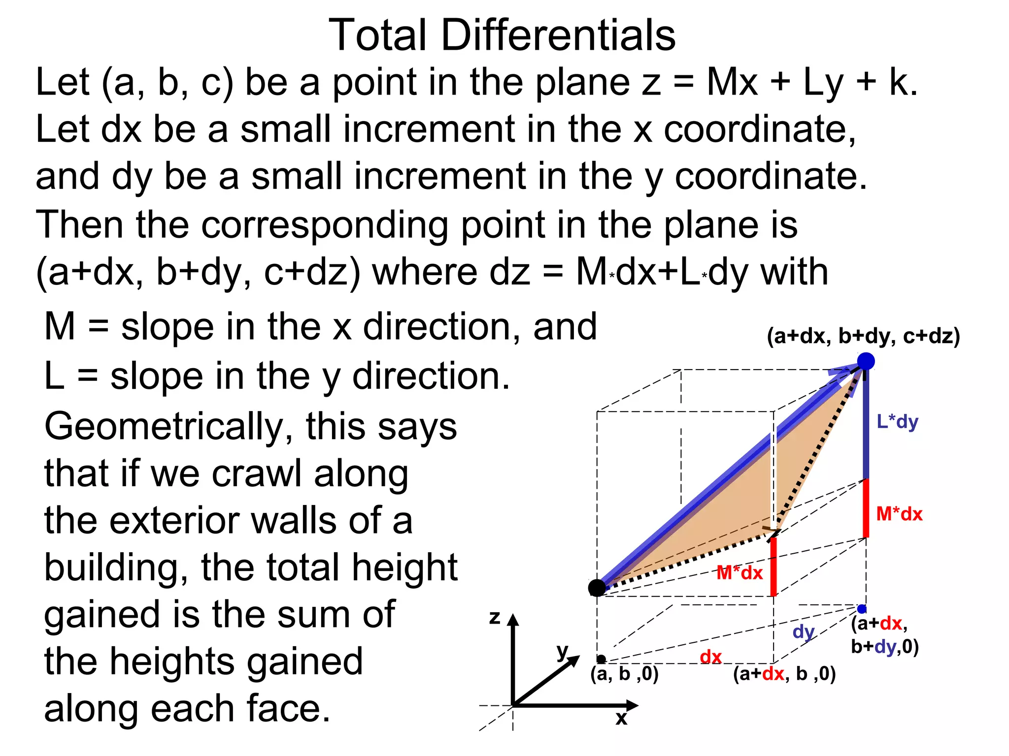
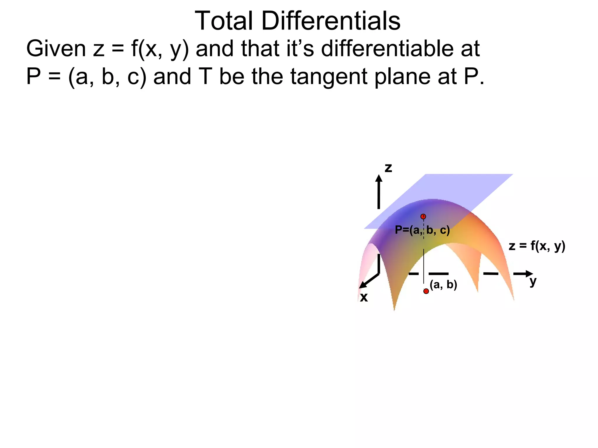
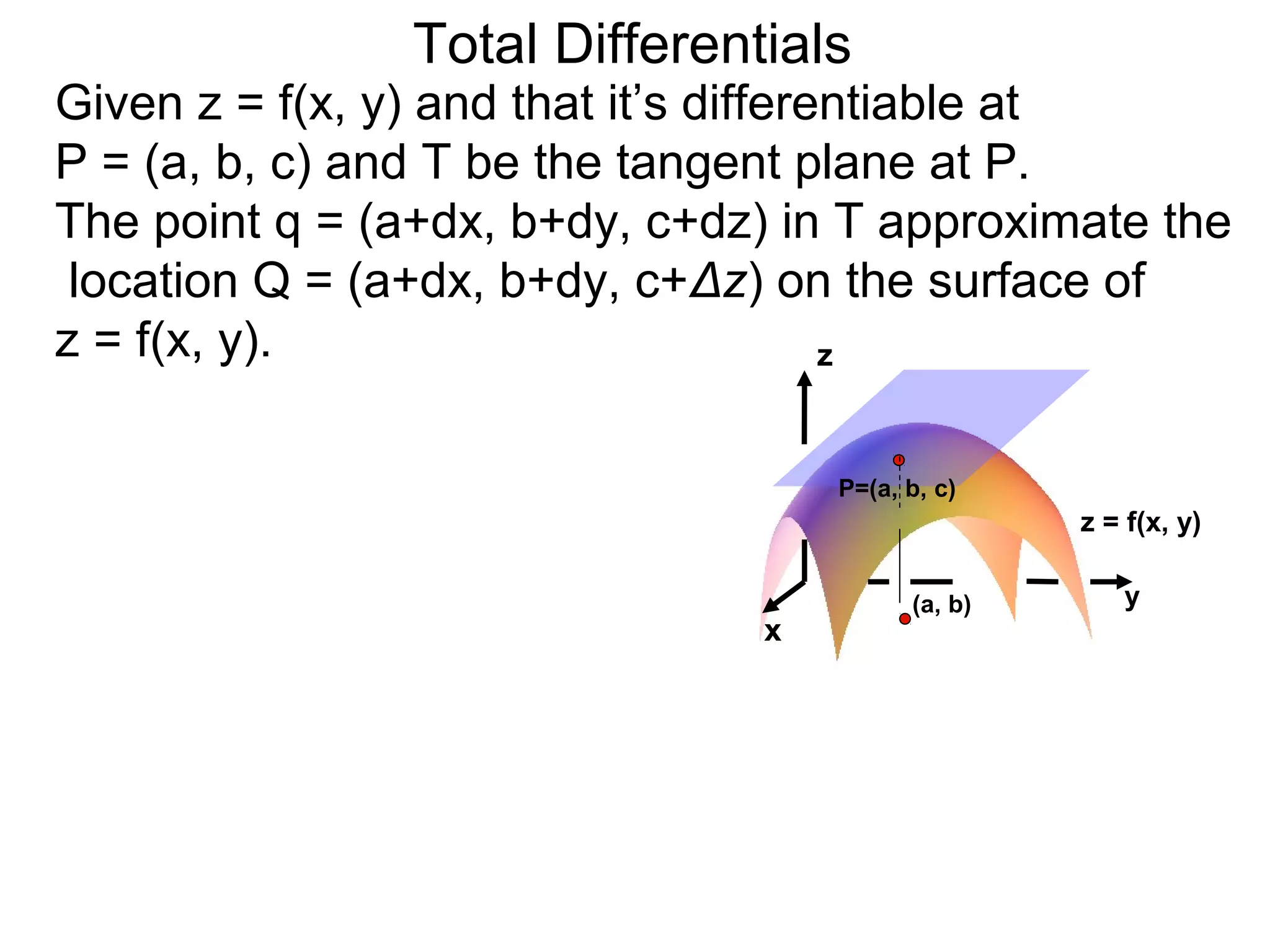
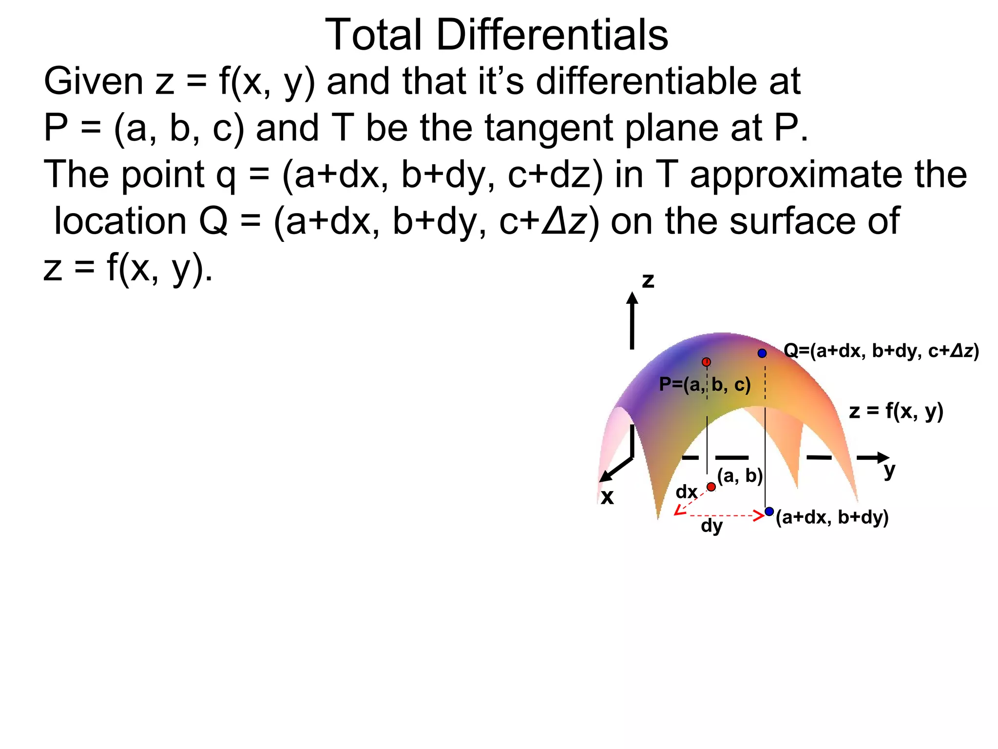
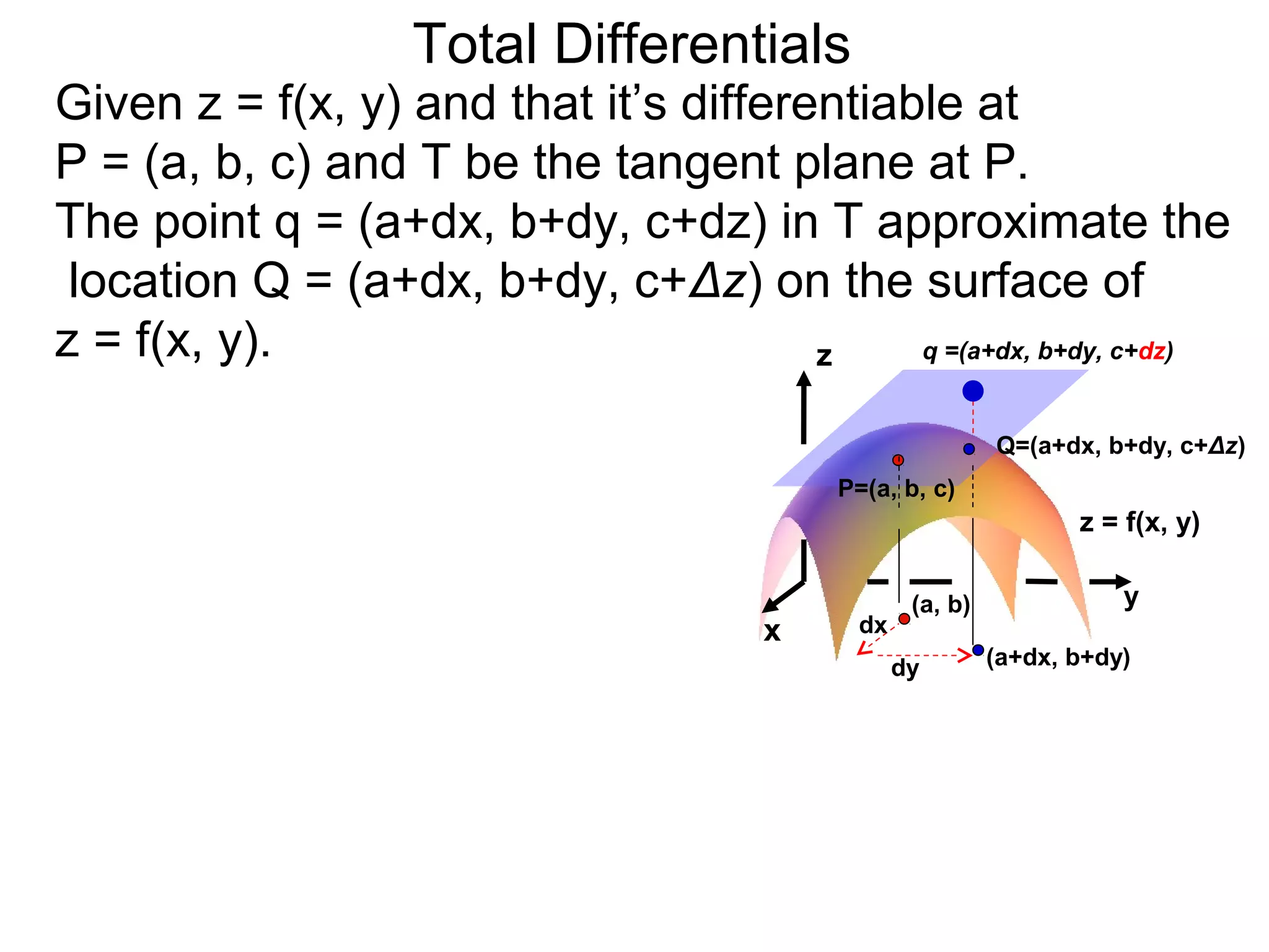
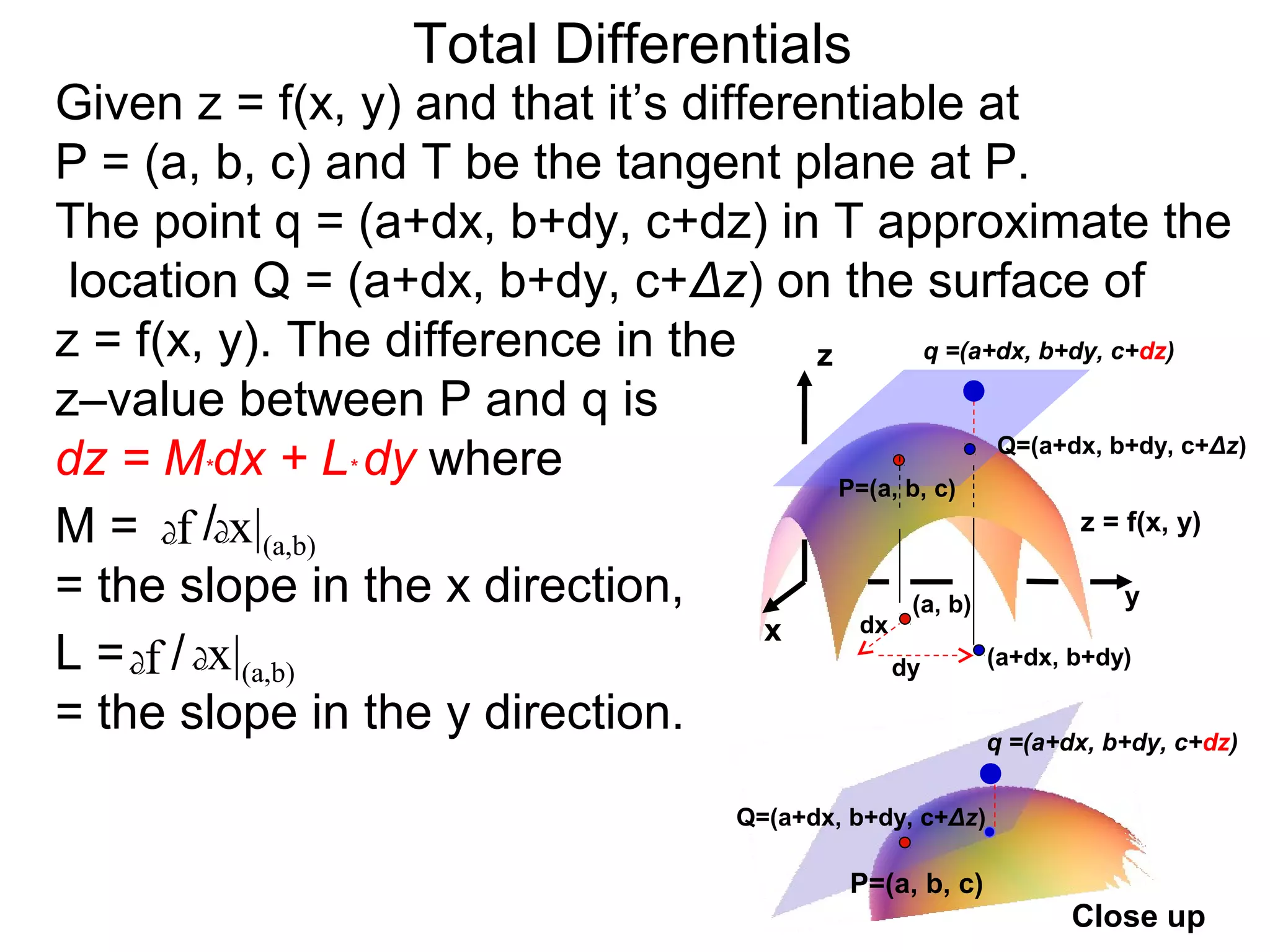
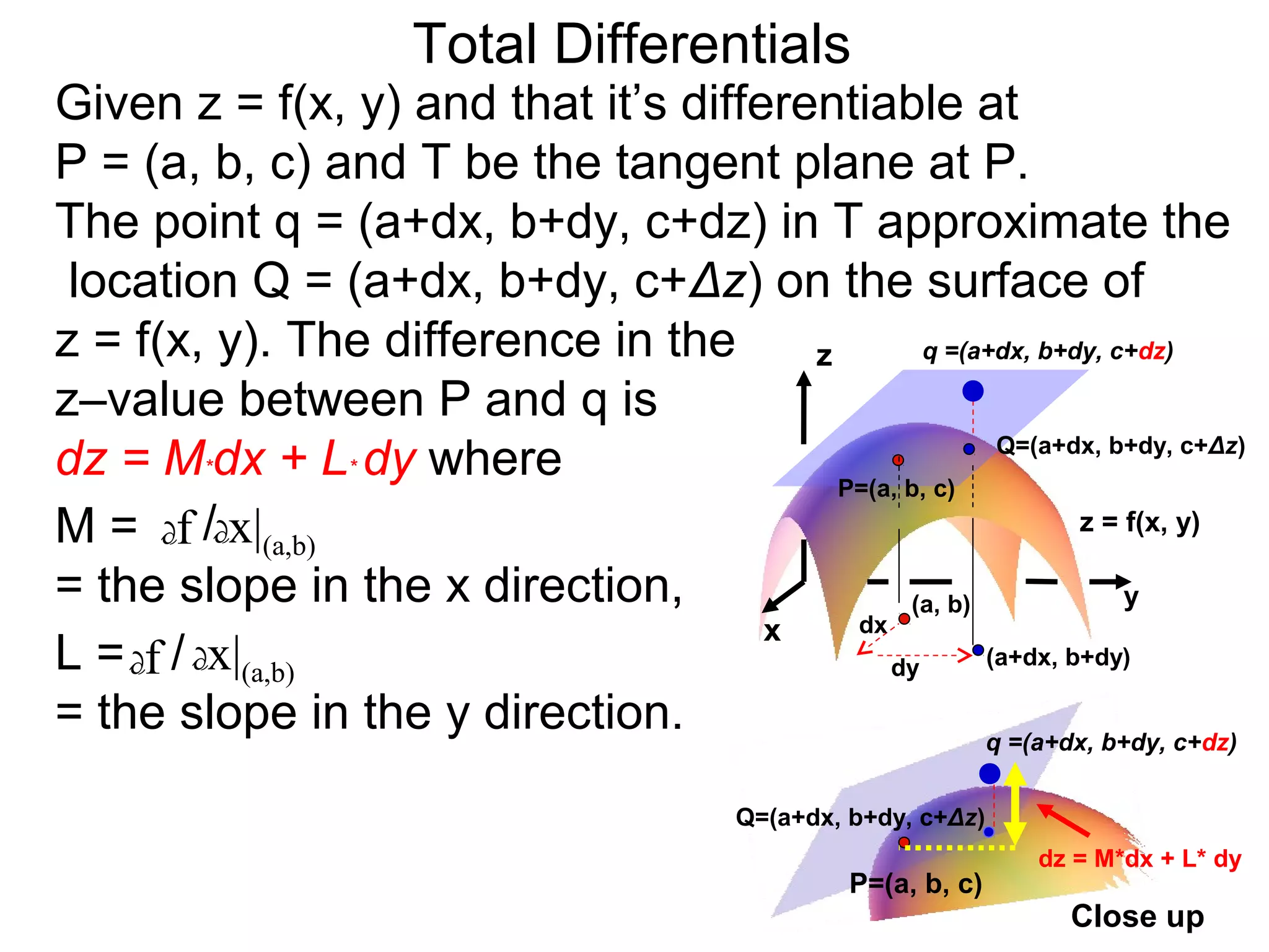
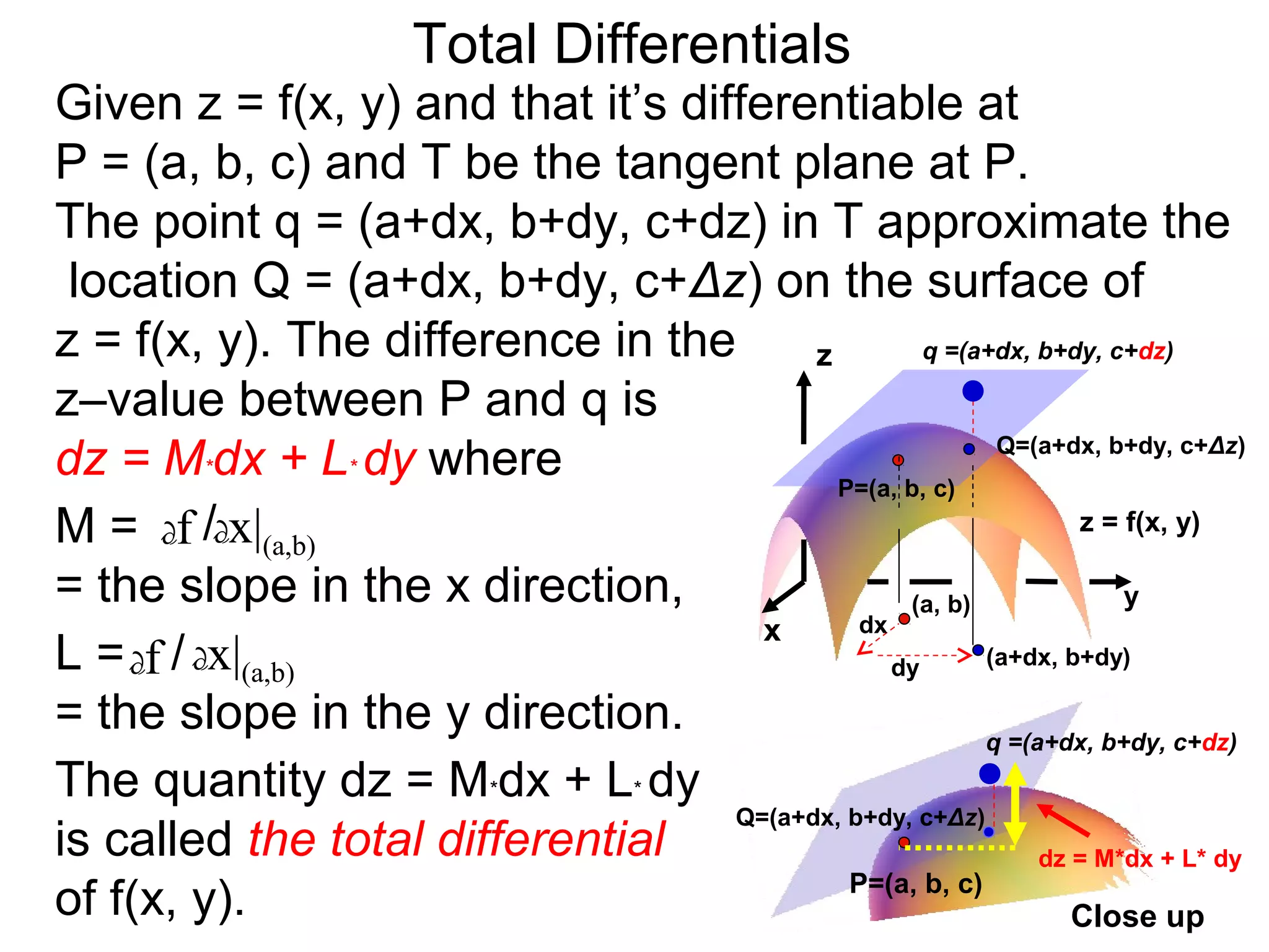
The document discusses tangent planes to surfaces. A surface is differentiable at a point if it is smooth and has a well-defined tangent plane at that point. The tangent plane approximates the surface near the point of tangency. To find the equation of the tangent plane, we calculate the partial derivatives of the surface function at the point to determine the slopes in the x- and y-directions. These slopes and the point define vectors in the tangent plane, and their cross product gives the normal vector. The equation of the tangent plane is then (z - c) = M(x - a) + L(y - b), where M and L are the partial derivatives and (a, b, c) is the

1. Tangent Planes

2. Tangent Planes
z
Recall that a surface z = f(x, y) is P =(a, b, c)
differentiable at a point P = (a, b, c)
or differentiable at p = (a, b), y
if it is smooth (no crease) and has a x
(a, b)
well defined tangent plane at P. A smooth point P and its tangent
plane.

3. Tangent Planes
z
Recall that a surface z = f(x, y) is P =(a, b, c)
differentiable at a point P = (a, b, c)
or differentiable at p = (a, b), y
if it is smooth (no crease) and has a x
(a, b)
well defined tangent plane at P. A smooth point P and its tangent
plane.
An "elementary function" is differentiable at a point p
if there is a circle centered at p and that all the partials
exist in this circle.

4. Tangent Planes
z
Recall that a surface z = f(x, y) is P =(a, b, c)
differentiable at a point P = (a, b, c)
or differentiable at p = (a, b), y
if it is smooth (no crease) and has a x
(a, b)
well defined tangent plane at P. A smooth point P and its tangent
plane.
An "elementary function" is differentiable at a point p
if there is a circle centered at p and that all the partials
exist in this circle.
Just as the tangent line to a curve at a point
approximates the curve around the point, the tangent
plane to a surface at a point P approximates the
surface around P.

5. Tangent Planes
z
Recall that a surface z = f(x, y) is P =(a, b, c)
differentiable at a point P = (a, b, c)
or differentiable at p = (a, b), y
if it is smooth (no crease) and has a x
(a, b)
well defined tangent plane at P. A smooth point P and its tangent
plane.
An "elementary function" is differentiable at a point p
if there is a circle centered at p and that all the partials
exist in this circle.
Just as the tangent line to a curve at a point
approximates the curve around the point, the tangent
plane to a surface at a point P approximates the
surface around P.
To find an equation for the tangent plane at P, we find
a normal vector N for the plane in the following

6. Tangent Planes
z
We note that a vector that sits in the <x, 0, z>
plane y = b has the form <x, 0, z>. y=b
x y

7. Tangent Planes
z
We note that a vector that sits in the <x, 0, z>
plane y = b has the form <x, 0, z>. y=b
Similarly, a vector that sits in the
x y
plane x = a has the form < 0, y, z>.

8. Tangent Planes
We note that a vector that sits in the <x, 0, z> z
plane y = b has the form <x, 0, z>. y=b
Similarly, a vector that sits in the
plane x = a has the form < 0, y, z>. x y
The tangent line to the y–trace at P = (a, b, c)

9. Tangent Planes
We note that a vector that sits in the <x, 0, z> z
plane y = b has the form <x, 0, z>. y=b
Similarly, a vector that sits in the
plane x = a has the form < 0, y, z>. x y
The tangent line to the y–trace at P = (a, b, c)
z
(a, b, c)
y
y=b
x

10. Tangent Planes
We note that a vector that sits in the <x, 0, z> z
plane y = b has the form <x, 0, z>. y=b
Similarly, a vector that sits in the
plane x = a has the form < 0, y, z>. x y
The tangent line to the y–trace at P = (a, b, c)
z
(a, b, c)
y
y=b
x

11. Tangent Planes
We note that a vector that sits in the <x, 0, z> z
plane y = b has the form <x, 0, z>. y=b
Similarly, a vector that sits in the
plane x = a has the form < 0, y, z>. x y
The tangent line to the y–trace at P = (a, b, c) is in the
tangent plane T and it has slope dz/dx|p = M.
z
(a, b, c)
y
y=b
x

12. Tangent Planes
We note that a vector that sits in the <x, 0, z> z
plane y = b has the form <x, 0, z>. y=b
Similarly, a vector that sits in the
plane x = a has the form < 0, y, z>. x y
The tangent line to the y–trace at P = (a, b, c) is in the
tangent plane T and it has slope dz/dx|p = M.
z
T
(a, b, c)
y
y=b
x

13. Tangent Planes
We note that a vector that sits in the <x, 0, z> z
plane y = b has the form <x, 0, z>. y=b
Similarly, a vector that sits in the
plane x = a has the form < 0, y, z>. x y
The tangent line to the y–trace at P = (a, b, c) is in the
tangent plane T and it has slope dz/dx|p = M.
z
T z (a, c) y=b
(a, b, c)
z = f(x, b)
x
y
y=b
x

14. Tangent Planes
We note that a vector that sits in the <x, 0, z> z
plane y = b has the form <x, 0, z>. y=b
Similarly, a vector that sits in the
plane x = a has the form < 0, y, z>. x y
The tangent line to the y–trace at P = (a, b, c) is in the
tangent plane T and it has slope dz/dx|p = M.
z
T z (a, c) y=b
1
(a, b, c)
z = f(x, b) M =d z
d x
x
y
y=b
x

15. Tangent Planes
We note that a vector that sits in the <x, 0, z> z
plane y = b has the form <x, 0, z>. y=b
Similarly, a vector that sits in the
plane x = a has the form < 0, y, z>. x y
The tangent line to the y–trace at P = (a, b, c) is in the
tangent plane T and it has slope dz/dx|p = M.
Hence the vector <1, 0, M> is in the tangent plane T.
z
T z (a, c) y=b
1
(a, b, c)
z = f(x, b) M =d z
d x
x
y
y=b
x

16. Tangent Planes
Similarly, the tangent plane must contain the tangent
line in the y-direction whose slope is dz/dy|p= L .
z
x=a
x y

17. Tangent Planes
Similarly, the tangent plane must contain the tangent
line in the y-direction whose slope is dz/dy|p= L .
z
T
(a, b, c)
x=a
x y

18. Tangent Planes
Similarly, the tangent plane must contain the tangent
line in the y-direction whose slope is dz/dy|p= L .
z
T z x=a
(a, b, c)
z = f(a,y)
1
(b, c)
L
x=a y
x y

19. Tangent Planes
Similarly, the tangent plane must contain the tangent
line in the y-direction whose slope is dz/dy|p= L .
Hence the vector <0, 1, L> is a tangent vector for the
x trace and <0, 1, L> is in T.
z
T z x=a
(a, b, c)
z = f(a,y)
1
(b, c)
L
x=a y
x y

20. Tangent Planes
Similarly, the tangent plane must contain the tangent
line in the y-direction whose slope is dz/dy|p= L .
Hence the vector <0, 1, L> is a tangent vector for the
x trace and <0, 1, L> is in T.
z
T z x=a
(a, b, c)
z = f(a,y)
1
(b, c)
L
x=a y
x y
z
Since <1, 0, M > and <0, 1, L>
are in T so their cross product
P
<1, 0, M> x <0, 1, L> = <–M, –L, 1>
is a normal vector to the tangent <1, 0, M>
<0, 1, L>
plane T. x y

21. Tangent Planes
Similarly, the tangent plane must contain the tangent
line in the y-direction whose slope is dz/dy|p= L .
Hence the vector <0, 1, L> is a tangent vector for the
x trace and <0, 1, L> is in T.
z
T z x=a
(a, b, c)
z = f(a,y)
1
(b, c)
L
x=a y
x y
z
Since <1, 0, M > and <0, 1, L> <–M, –L, 1>
are in T so their cross product
P
<1, 0, M> x <0, 1, L> = <–M, –L, 1>
is a normal vector to the tangent <1, 0, M>
<0, 1, L>
plane T. x y

22. Tangent Planes
Equation of The Tangent Plane. Given that a normal
vector is <–M, –L, 1>, an equation of the tangent plane
at P = (a, b, c) is (z – c) = M(x – a) + L(y – b)
where with M = dz / dx|p and L = dz / dy|p <–M, –L, 1>
P
<0, 1, L>
<1, 0, M>
x y

23. Tangent Planes
Equation of The Tangent Plane. Given that a normal
vector is <–M, –L, 1>, an equation of the tangent plane
at P = (a, b, c) is (z – c) = M(x – a) + L(y – b)
where with M = dz / dx|p and L = dz / dy|p <–M, –L, 1>
Example A. Find the equation of the P
tangent plane for z = √49 – x2 – y2 at <0, 1, L>
<1, 0, M>
(2, 3, 6). x y

24. Tangent Planes
Equation of The Tangent Plane. Given that a normal
vector is <–M, –L, 1>, an equation of the tangent plane
at P = (a, b, c) is (z – c) = M(x – a) + L(y – b)
where with M = dz / dx|p and L = dz / dy|p <–M, –L, 1>
Example A. Find the equation of the P
tangent plane for z = √49 – x2 – y2 at <0, 1, L>
<1, 0, M>
(2, 3, 6). x y
fx(P)= –x/√49 – x2 – y2, fy(P)= –x/√49 – x2 – y2,

25. Tangent Planes
Equation of The Tangent Plane. Given that a normal
vector is <–M, –L, 1>, an equation of the tangent plane
at P = (a, b, c) is (z – c) = M(x – a) + L(y – b)
where with M = dz / dx|p and L = dz / dy|p <–M, –L, 1>
Example A. Find the equation of the P
tangent plane for z = √49 – x2 – y2 at <0, 1, L>
<1, 0, M>
(2, 3, 6). x y
fx(P)= –x/√49 – x2 – y2, fy(P)= –x/√49 – x2 – y2,
Hence M = fx(2, 3) = –1/3, and L = fy(2, 3) = –1/2

26. Tangent Planes
Equation of The Tangent Plane. Given that a normal
vector is <–M, –L, 1>, an equation of the tangent plane
at P = (a, b, c) is (z – c) = M(x – a) + L(y – b)
where with M = dz / dx|p and L = dz / dy|p <–M, –L, 1>
Example A. Find the equation of the P
tangent plane for z = √49 – x2 – y2 at <0, 1, L>
<1, 0, M>
(2, 3, 6). x y
fx(P)= –x/√49 – x2 – y2, fy(P)= –x/√49 – x2 – y2,
Hence M = fx(2, 3) = –1/3, and L = fy(2, 3) = –1/2
So the equation of the tangent plane at (2,3,6) is
(z – 6) = –1/3(x – 2) – 1/2 (y – 3)
or that 2x + 3y + 6z = 49.

27. Tangent Planes
Equation of The Tangent Plane. Given that a normal
vector is <–M, –L, 1>, an equation of the tangent plane
at P = (a, b, c) is (z – c) = M(x – a) + L(y – b)
where with M = dz / dx|p and L = dz / dy|p <–M, –L, 1>
Example A. Find the equation of the P
tangent plane for z = √49 – x2 – y2 at <0, 1, L>
<1, 0, M>
(2, 3, 6). x y
fx(P)= –x/√49 – x2 – y2, fy(P)= –x/√49 – x2 – y2,
Hence M = fx(2, 3) = –1/3, and L = fy(2, 3) = –1/2
So the equation of the tangent plane at (2,3,6) is
(z – 6) = –1/3(x – 2) – 1/2 (y – 3)
or that 2x + 3y + 6z = 49.
Use a graphing software to verity this result.

28. Total Differentials
Let y = f(x), we write Δx as dx to represent a small
change in the value x, and we write Δy = f(x + Δx) – f(x)
as the corresponding change in the output y.

29. Total Differentials
Let y = f(x), we write Δx as dx to represent a small
change in the value x, and we write Δy = f(x + Δx) – f(x)
as the corresponding change in the output y.
If f(x) is differentiable at x = a, then
f(a + dx) ≈ f(a) + f'(a)*dx where f'(a)*dx ≈ Δy.

30. Total Differentials
Let y = f(x), we write Δx as dx to represent a small
change in the value x, and we write Δy = f(x + Δx) – f(x)
as the corresponding change in the output y.
If f(x) is differentiable at x = a, then
f(a + dx) ≈ f(a) + f'(a)*dx where f'(a)*dx ≈ Δy.
y=f(x)
f(a)
a

31. Total Differentials
Let y = f(x), we write Δx as dx to represent a small
change in the value x, and we write Δy = f(x + Δx) – f(x)
as the corresponding change in the output y.
If f(x) is differentiable at x = a, then
f(a + dx) ≈ f(a) + f'(a)*dx where f'(a)*dx ≈ Δy.
y=f(x)
f(a)
f(a+dx)
dx
a a+dx

32. Total Differentials
Let y = f(x), we write Δx as dx to represent a small
change in the value x, and we write Δy = f(x + Δx) – f(x)
as the corresponding change in the output y.
If f(x) is differentiable at x = a, then
f(a + dx) ≈ f(a) + f'(a)*dx where f'(a)*dx ≈ Δy.
Δy
y=f(x)
f(a)
f(a+dx)
dx
a a+dx

33. Total Differentials
Let y = f(x), we write Δx as dx to represent a small
change in the value x, and we write Δy = f(x + Δx) – f(x)
as the corresponding change in the output y.
If f(x) is differentiable at x = a, then
f(a + dx) ≈ f(a) + f'(a)*dx where f'(a)*dx ≈ Δy.
Δy
y=f(x)
f(a)
f(a+dx)
dx
a a+dx

34. Total Differentials
Let y = f(x), we write Δx as dx to represent a small
change in the value x, and we write Δy = f(x + Δx) – f(x)
as the corresponding change in the output y.
If f(x) is differentiable at x = a, then
f(a + dx) ≈ f(a) + f'(a)*dx where f'(a)*dx ≈ Δy. f'(a) dx=dy *
Δy
y=f(x)
f(a)
f(a+dx)
dx
a a+dx

35. Total Differentials
Let y = f(x), we write Δx as dx to represent a small
change in the value x, and we write Δy = f(x + Δx) – f(x)
as the corresponding change in the output y.
If f(x) is differentiable at x = a, then
f(a + dx) ≈ f(a) + f'(a)*dx where f'(a)*dx ≈ Δy. f'(a) dx=dy *
Δy
y=f(x)
f(a)
f(a+dx) f(a)+ f'(a)*dx
dx
a a+dx

36. Total Differentials
Let y = f(x), we write Δx as dx to represent a small
change in the value x, and we write Δy = f(x + Δx) – f(x)
as the corresponding change in the output y.
If f(x) is differentiable at x = a, then
f(a + dx) ≈ f(a) + f'(a)*dx where f'(a)*dx ≈ Δy. f'(a) dx=dy *
We call dx “the differential of x”, Δy
y=f(x)
and we write the approximation
f'(x)dx as dy which is called f(a)
f(a+dx) f(a)+ f'(a)*dx
“the differential of y”. We have that dx
f'(a)*dx = dy ≈ Δy. a a+dx

37. Total Differentials
Let y = f(x), we write Δx as dx to represent a small
change in the value x, and we write Δy = f(x + Δx) – f(x)
as the corresponding change in the output y.
If f(x) is differentiable at x = a, then
f(a + dx) ≈ f(a) + f'(a)*dx where f'(a)*dx ≈ Δy. f'(a) dx=dy *
We call dx “the differential of x”, Δy
y=f(x)
and we write the approximation
f'(x)dx as dy which is called f(a)
f(a+dx) f(a)+ f'(a)*dx
“the differential of y”. We have that dx
f'(a)*dx = dy ≈ Δy. a a+dx
We use dy, which is easier to calculate, to estimates
the change in the output.

38. Total Differentials
Let y = f(x), we write Δx as dx to represent a small
change in the value x, and we write Δy = f(x + Δx) – f(x)
as the corresponding change in the output y.
If f(x) is differentiable at x = a, then
f(a + dx) ≈ f(a) + f'(a)*dx where f'(a)*dx ≈ Δy. f'(a) dx=dy *
We call dx “the differential of x”, Δy
y=f(x)
and we write the approximation
f'(x)dx as dy which is called f(a)
f(a+dx) f(a)+ f'(a)*dx
“the differential of y”. We have that dx
f'(a)*dx = dy ≈ Δy. a a+dx
We use dy, which is easier to calculate, to estimates
the change in the output. For example, let y = f(x) = x 2,
at (3, 9), dy = f'(3) dx = 6 dx,.

39. Total Differentials
Let y = f(x), we write Δx as dx to represent a small
change in the value x, and we write Δy = f(x + Δx) – f(x)
as the corresponding change in the output y.
If f(x) is differentiable at x = a, then
f(a + dx) ≈ f(a) + f'(a)*dx where f'(a)*dx ≈ Δy. f'(a) dx=dy *
We call dx “the differential of x”, Δy
y=f(x)
and we write the approximation
f'(x)dx as dy which is called f(a)
f(a+dx) f(a)+ f'(a)*dx
“the differential of y”. We have that dx
f'(a)*dx = dy ≈ Δy. a a+dx
We use dy, which is easier to calculate, to estimates
the change in the output. For example, let y = f(x) = x 2,
at (3, 9), dy = f'(3) dx = 6 dx. So if dx = 0.01,
then dy = 0.06.

40. Total Differentials
Let y = f(x), we write Δx as dx to represent a small
change in the value x, and we write Δy = f(x + Δx) – f(x)
as the corresponding change in the output y.
If f(x) is differentiable at x = a, then
f(a + dx) ≈ f(a) + f'(a)*dx where f'(a)*dx ≈ Δy. f'(a) dx=dy *
We call dx “the differential of x”, Δy
y=f(x)
and we write the approximation
f'(x)dx as dy which is called f(a)
f(a+dx) f(a)+ f'(a)*dx
“the differential of y”. We have that dx
f'(a)*dx = dy ≈ Δy. a a+dx
We use dy, which is easier to calculate, to estimates
the change in the output. For example, let y = f(x) = x 2,
at (3, 9), dy = f'(3) dx = 6 dx. So if dx = 0.01,
then dy = 0.06. Note that Δy = f(3.01) – f(3) = 0.0601.

41. Total Differentials
Let (a, b, c) be a point in the plane z = Mx + Ly + k.
z
y
(a, b ,0)
x

42. Total Differentials
Let (a, b, c) be a point in the plane z = Mx + Ly + k.
Let dx be a small increment in the x coordinate,
and dy be a small increment in the y coordinate.
z (a+dx,
dy
y b+dy,0)
dx
(a, b ,0) (a+dx, b ,0)
x

43. Total Differentials
Let (a, b, c) be a point in the plane z = Mx + Ly + k.
Let dx be a small increment in the x coordinate,
and dy be a small increment in the y coordinate.
Then the corresponding point in the plane is
(a+dx, b+dy, c+dz) where dz = M*dx+L*dy
(a+dx, b+dy, c+dz)
z (a+dx,
dy
y b+dy,0)
dx
(a, b ,0) (a+dx, b ,0)
x

44. Total Differentials
Let (a, b, c) be a point in the plane z = Mx + Ly + k.
Let dx be a small increment in the x coordinate,
and dy be a small increment in the y coordinate.
Then the corresponding point in the plane is
(a+dx, b+dy, c+dz) where dz = M*dx+L*dy with
M = slope in the x direction, (a+dx, b+dy, c+dz)
M*dx
z (a+dx,
dy
y b+dy,0)
dx
(a, b ,0) (a+dx, b ,0)
x

45. Total Differentials
Let (a, b, c) be a point in the plane z = Mx + Ly + k.
Let dx be a small increment in the x coordinate,
and dy be a small increment in the y coordinate.
Then the corresponding point in the plane is
(a+dx, b+dy, c+dz) where dz = M*dx+L*dy with
M = slope in the x direction, and (a+dx, b+dy, c+dz)
L = slope in the y direction.
L*dy
M*dx
M*dx
z (a+dx,
dy
y b+dy,0)
dx
(a, b ,0) (a+dx, b ,0)
x

46. Total Differentials
Let (a, b, c) be a point in the plane z = Mx + Ly + k.
Let dx be a small increment in the x coordinate,
and dy be a small increment in the y coordinate.
Then the corresponding point in the plane is
(a+dx, b+dy, c+dz) where dz = M*dx+L*dy with
M = slope in the x direction, and (a+dx, b+dy, c+dz)
L = slope in the y direction.
L*dy
dz
M*dx
M*dx
z (a+dx,
dy
y b+dy,0)
dx
(a, b ,0) (a+dx, b ,0)
x

47. Total Differentials
Let (a, b, c) be a point in the plane z = Mx + Ly + k.
Let dx be a small increment in the x coordinate,
and dy be a small increment in the y coordinate.
Then the corresponding point in the plane is
(a+dx, b+dy, c+dz) where dz = M*dx+L*dy with
M = slope in the x direction, and (a+dx, b+dy, c+dz)
L = slope in the y direction.
Geometrically, this says L*dy
that if we crawl along
the exterior walls of a M*dx
building, the total height M*dx
gained is the sum of z
dy (a+dx,
y b+dy,0)
the heights gained (a, b ,0)
dx
(a+dx, b ,0)
along each face. x

48. Total Differentials
Given z = f(x, y) and that it’s differentiable at
P = (a, b, c) and T be the tangent plane at P.
z
P=(a, b, c)
z = f(x, y)
(a, b) y
x

49. Total Differentials
Given z = f(x, y) and that it’s differentiable at
P = (a, b, c) and T be the tangent plane at P.
The point q = (a+dx, b+dy, c+dz) in T approximate the
location Q = (a+dx, b+dy, c+Δz) on the surface of
z = f(x, y). z
P=(a, b, c)
z = f(x, y)
(a, b) y
x

50. Total Differentials
Given z = f(x, y) and that it’s differentiable at
P = (a, b, c) and T be the tangent plane at P.
The point q = (a+dx, b+dy, c+dz) in T approximate the
location Q = (a+dx, b+dy, c+Δz) on the surface of
z = f(x, y). z
Q=(a+dx, b+dy, c+Δz)
P=(a, b, c)
z = f(x, y)
(a, b) y
x dx
dy (a+dx, b+dy)

51. Total Differentials
Given z = f(x, y) and that it’s differentiable at
P = (a, b, c) and T be the tangent plane at P.
The point q = (a+dx, b+dy, c+dz) in T approximate the
location Q = (a+dx, b+dy, c+Δz) on the surface of
z = f(x, y). z q =(a+dx, b+dy, c+dz)
Q=(a+dx, b+dy, c+Δz)
P=(a, b, c)
z = f(x, y)
(a, b) y
x dx
dy (a+dx, b+dy)

52. Total Differentials
Given z = f(x, y) and that it’s differentiable at
P = (a, b, c) and T be the tangent plane at P.
The point q = (a+dx, b+dy, c+dz) in T approximate the
location Q = (a+dx, b+dy, c+Δz) on the surface of
z = f(x, y). The difference in the z q =(a+dx, b+dy, c+dz)
z–value between P and q is
dz = M*dx + L* dy where P=(a, b, c)
Q=(a+dx, b+dy, c+Δz)
M = df /dx|(a,b) z = f(x, y)
= the slope in the x direction, (a, b) y
x dx
L = df / dx|(a,b) dy (a+dx, b+dy)
= the slope in the y direction. q =(a+dx, b+dy, c+dz)
Q=(a+dx, b+dy, c+Δz)
P=(a, b, c)
Close up

53. Total Differentials
Given z = f(x, y) and that it’s differentiable at
P = (a, b, c) and T be the tangent plane at P.
The point q = (a+dx, b+dy, c+dz) in T approximate the
location Q = (a+dx, b+dy, c+Δz) on the surface of
z = f(x, y). The difference in the z q =(a+dx, b+dy, c+dz)
z–value between P and q is
dz = M*dx + L* dy where P=(a, b, c)
Q=(a+dx, b+dy, c+Δz)
M = df /dx|(a,b) z = f(x, y)
= the slope in the x direction, (a, b) y
x dx
L = df / dx|(a,b) dy (a+dx, b+dy)
= the slope in the y direction. q =(a+dx, b+dy, c+dz)
Q=(a+dx, b+dy, c+Δz)
dz = M*dx + L* dy
P=(a, b, c)
Close up

54. Total Differentials
Given z = f(x, y) and that it’s differentiable at
P = (a, b, c) and T be the tangent plane at P.
The point q = (a+dx, b+dy, c+dz) in T approximate the
location Q = (a+dx, b+dy, c+Δz) on the surface of
z = f(x, y). The difference in the z q =(a+dx, b+dy, c+dz)
z–value between P and q is
dz = M*dx + L* dy where P=(a, b, c)
Q=(a+dx, b+dy, c+Δz)
M = df /dx|(a,b) z = f(x, y)
= the slope in the x direction, (a, b) y
x dx
L = df / dx|(a,b) dy (a+dx, b+dy)
= the slope in the y direction. q =(a+dx, b+dy, c+dz)
The quantity dz = M*dx + L* dy
Q=(a+dx, b+dy, c+Δz)
is called the total differential dz = M*dx + L* dy
P=(a, b, c)
of f(x, y). Close up

55. Total Differentials
Example B. Approximate the value of x3y – x2y2
at (x, y) = (1.03, 2.94) using the differentials.

56. Total Differentials
Example B. Approximate the value of x3y – x2y2
at (x, y) = (1.03, 2.94) using the differentials.
Let’s set z = f(x,y) = x3y – x2y2.

57. Total Differentials
Example B. Approximate the value of x3y – x2y2
at (x, y) = (1.03, 2.94) using the differentials.
Let’s set z = f(x,y) = x3y – x2y2. Select P = (1, 3)
which is close to (1.03, 2.94) and easy to evaluate.

58. Total Differentials
Example B. Approximate the value of x3y – x2y2
at (x, y) = (1.03, 2.94) using the differentials.
Let’s set z = f(x,y) = x3y – x2y2. Select P = (1, 3)
which is close to (1.03, 2.94) and easy to evaluate.
At P = (1, 3), z = 3 – 9 = –6.

59. Total Differentials
Example B. Approximate the value of x3y – x2y2
at (x, y) = (1.03, 2.94) using the differentials.
Let’s set z = f(x,y) = x3y – x2y2. Select P = (1, 3)
which is close to (1.03, 2.94) and easy to evaluate.
At P = (1, 3), z = 3 – 9 = –6. To find an approximate
value of f(1.03, 2.94), we calculate the z–value of
(1.03, 2.94) on the tangent plane that touches (1, 3, 6).

60. Total Differentials
Example B. Approximate the value of x3y – x2y2
at (x, y) = (1.03, 2.94) using the differentials.
Let’s set z = f(x,y) = x3y – x2y2. Select P = (1, 3)
which is close to (1.03, 2.94) and easy to evaluate.
At P = (1, 3), z = 3 – 9 = –6. To find an approximate
value of f(1.03, 2.94), we calculate the z–value of
(1.03, 2.94) on the tangent plane that touches (1, 3, 6).
From (1, 3) to (1.03, 2.94), dx = 0.03 and dy = –0.06.

61. Total Differentials
Example B. Approximate the value of x3y – x2y2
at (x, y) = (1.03, 2.94) using the differentials.
Let’s set z = f(x,y) = x3y – x2y2. Select P = (1, 3)
which is close to (1.03, 2.94) and easy to evaluate.
At P = (1, 3), z = 3 – 9 = –6. To find an approximate
value of f(1.03, 2.94), we calculate the z–value of
(1.03, 2.94) on the tangent plane that touches (1, 3, 6).
From (1, 3) to (1.03, 2.94), dx = 0.03 and dy = –0.06.
The partials at (1, 3), M = fx|(1,3)= 3x2y – 2xy2|(1,3) = –9,

62. Total Differentials
Example B. Approximate the value of x3y – x2y2
at (x, y) = (1.03, 2.94) using the differentials.
Let’s set z = f(x,y) = x3y – x2y2. Select P = (1, 3)
which is close to (1.03, 2.94) and easy to evaluate.
At P = (1, 3), z = 3 – 9 = –6. To find an approximate
value of f(1.03, 2.94), we calculate the z–value of
(1.03, 2.94) on the tangent plane that touches (1, 3, 6).
From (1, 3) to (1.03, 2.94), dx = 0.03 and dy = –0.06.
The partials at (1, 3), M = fx|(1,3)= 3x2y – 2xy2|(1,3) = –9,
and L = fy|(1,3)= x3 – 2x2y|(1,3) = –5.

63. Total Differentials
Example B. Approximate the value of x3y – x2y2
at (x, y) = (1.03, 2.94) using the differentials.
Let’s set z = f(x,y) = x3y – x2y2. Select P = (1, 3)
which is close to (1.03, 2.94) and easy to evaluate.
At P = (1, 3), z = 3 – 9 = –6. To find an approximate
value of f(1.03, 2.94), we calculate the z–value of
(1.03, 2.94) on the tangent plane that touches (1, 3, 6).
From (1, 3) to (1.03, 2.94), dx = 0.03 and dy = –0.06.
The partials at (1, 3), M = fx|(1,3)= 3x2y – 2xy2|(1,3) = –9,
and L = fy|(1,3)= x3 – 2x2y|(1,3) = –5.
Hence dz = M*dx + L* dy

64. Total Differentials
Example B. Approximate the value of x3y – x2y2
at (x, y) = (1.03, 2.94) using the differentials.
Let’s set z = f(x,y) = x3y – x2y2. Select P = (1, 3)
which is close to (1.03, 2.94) and easy to evaluate.
At P = (1, 3), z = 3 – 9 = –6. To find an approximate
value of f(1.03, 2.94), we calculate the z–value of
(1.03, 2.94) on the tangent plane that touches (1, 3, 6).
From (1, 3) to (1.03, 2.94), dx = 0.03 and dy = –0.06.
The partials at (1, 3), M = fx|(1,3)= 3x2y – 2xy2|(1,3) = –9,
and L = fy|(1,3)= x3 – 2x2y|(1,3) = –5.
Hence dz = M*dx + L* dy = –9(0.03) – 5(–0.06) = 0.03,

65. Total Differentials
Example B. Approximate the value of x3y – x2y2
at (x, y) = (1.03, 2.94) using the differentials.
Let’s set z = f(x,y) = x3y – x2y2. Select P = (1, 3)
which is close to (1.03, 2.94) and easy to evaluate.
At P = (1, 3), z = 3 – 9 = –6. To find an approximate
value of f(1.03, 2.94), we calculate the z–value of
(1.03, 2.94) on the tangent plane that touches (1, 3, 6).
From (1, 3) to (1.03, 2.94), dx = 0.03 and dy = –0.06.
The partials at (1, 3), M = fx|(1,3)= 3x2y – 2xy2|(1,3) = –9,
and L = fy|(1,3)= x3 – 2x2y|(1,3) = –5.
Hence dz = M*dx + L* dy = –9(0.03) – 5(–0.06) = 0.03,
so f(1.03, 2.94) ≈ f(1, 3) + dz = –6 + 0.03 = –5.970.

66. Total Differentials
Example B. Approximate the value of x3y – x2y2
at (x, y) = (1.03, 2.94) using the differentials.
Let’s set z = f(x,y) = x3y – x2y2. Select P = (1, 3)
which is close to (1.03, 2.94) and easy to evaluate.
At P = (1, 3), z = 3 – 9 = –6. To find an approximate
value of f(1.03, 2.94), we calculate the z–value of
(1.03, 2.94) on the tangent plane that touches (1, 3, 6).
From (1, 3) to (1.03, 2.94), dx = 0.03 and dy = –0.06.
The partials at (1, 3), M = fx|(1,3)= 3x2y – 2xy2|(1,3) = –9,
and L = fy|(1,3)= x3 – 2x2y|(1,3) = –5.
Hence dz = M*dx + L* dy = –9(0.03) – 5(–0.06) = 0.03,
so f(1.03, 2.94) ≈ f(1, 3) + dz = –6 + 0.03 = –5.970.
The calculator answer of f(1.03, 2.94) ≈ –5.957.