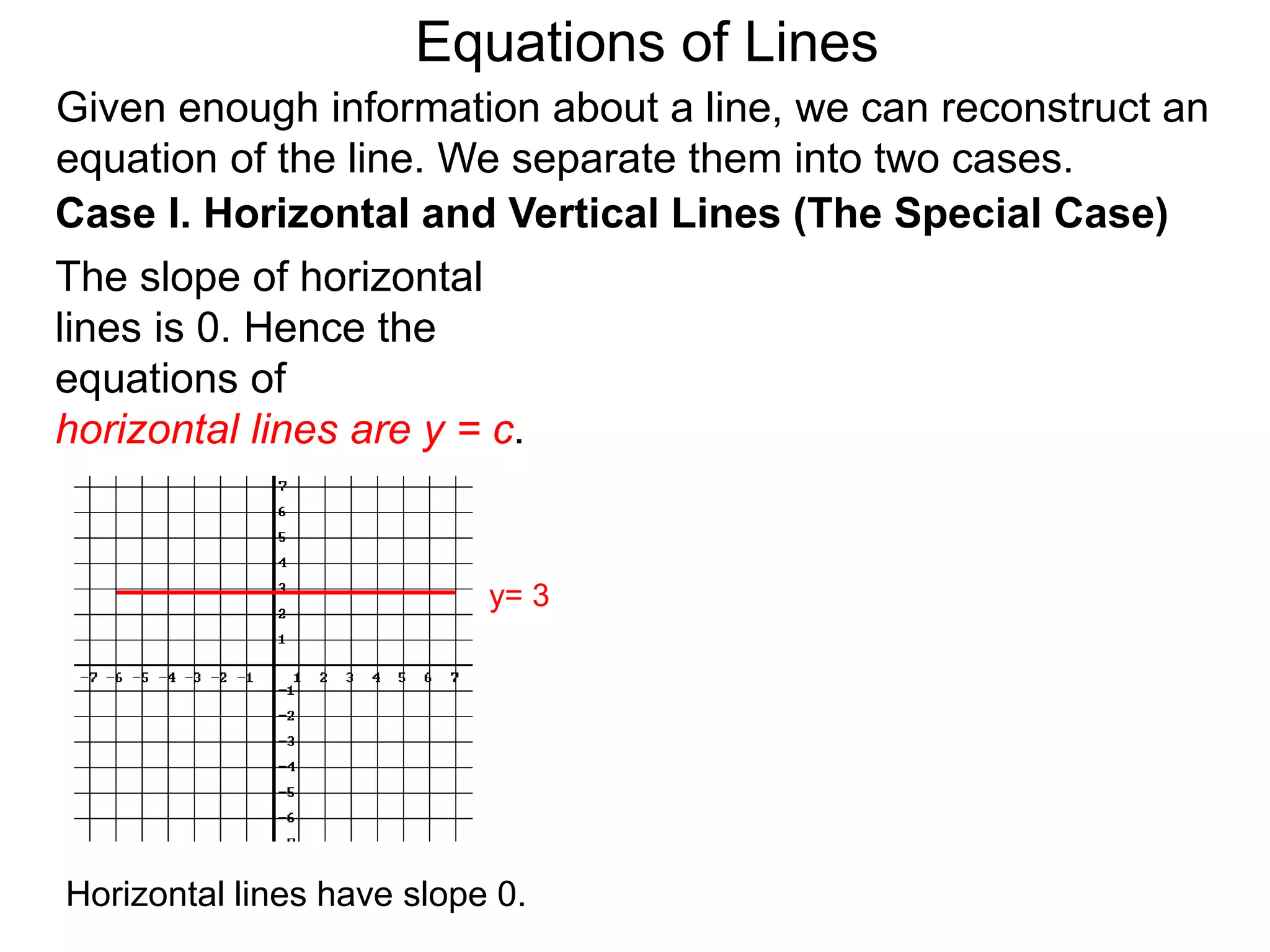
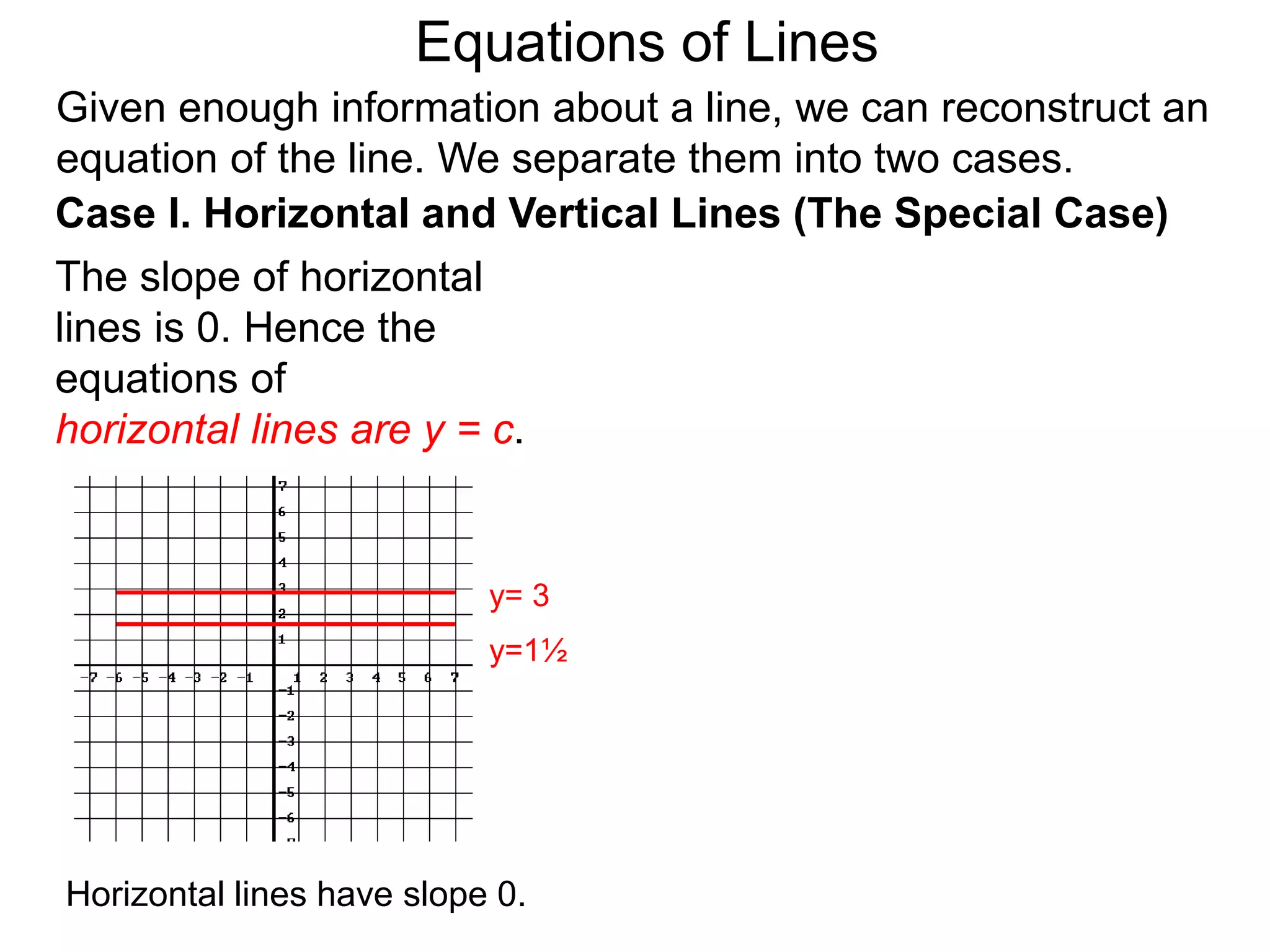
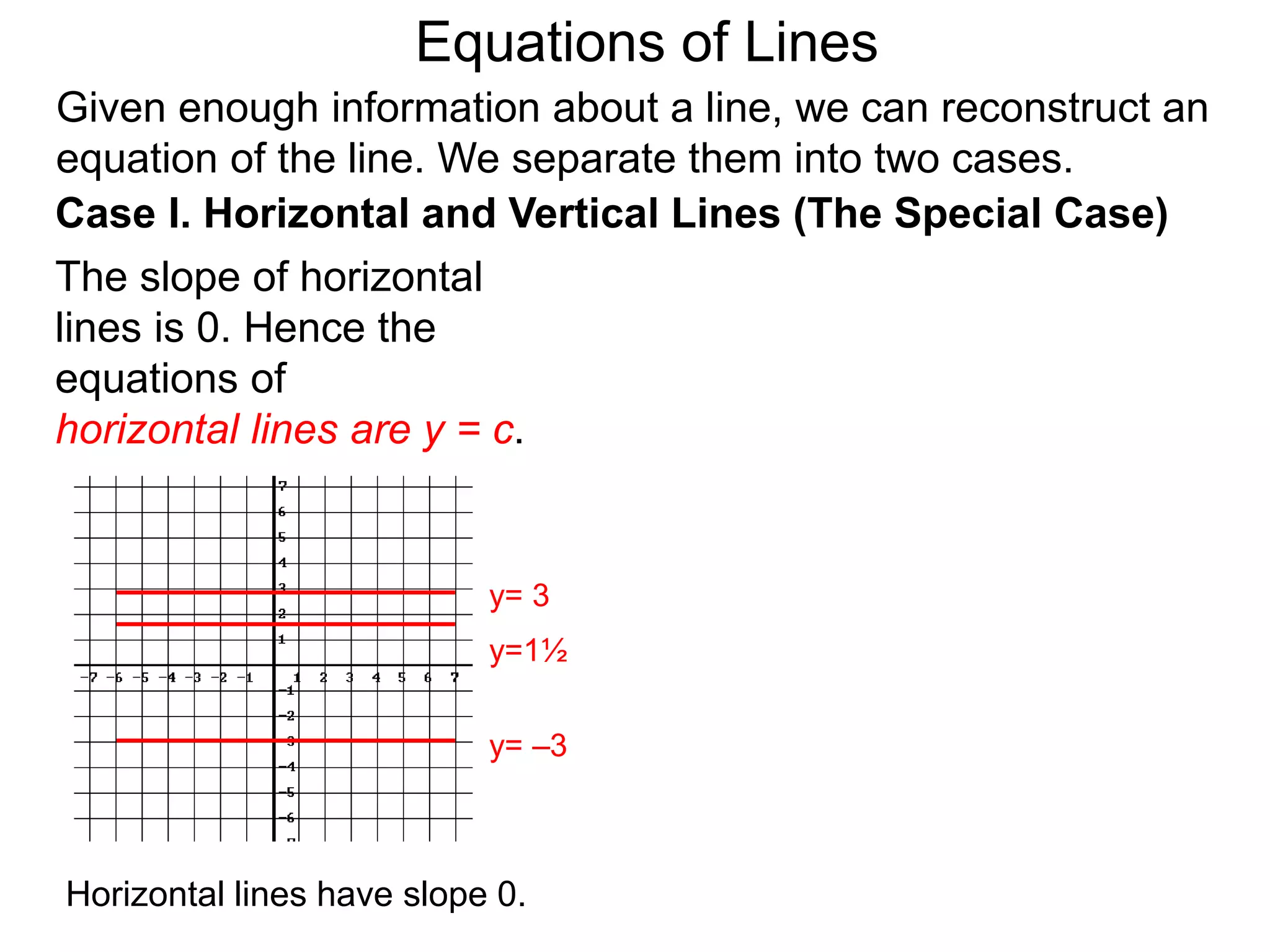
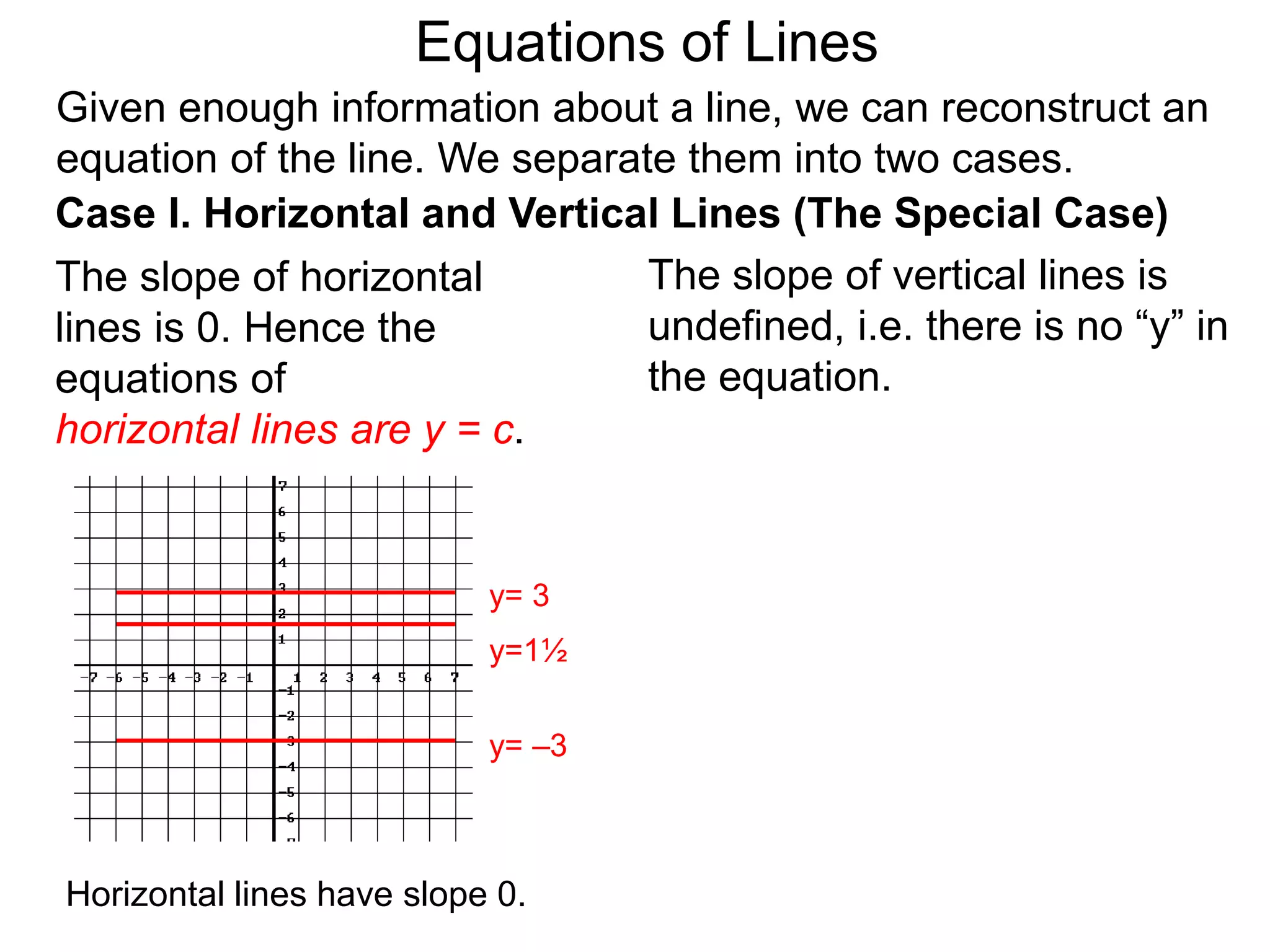
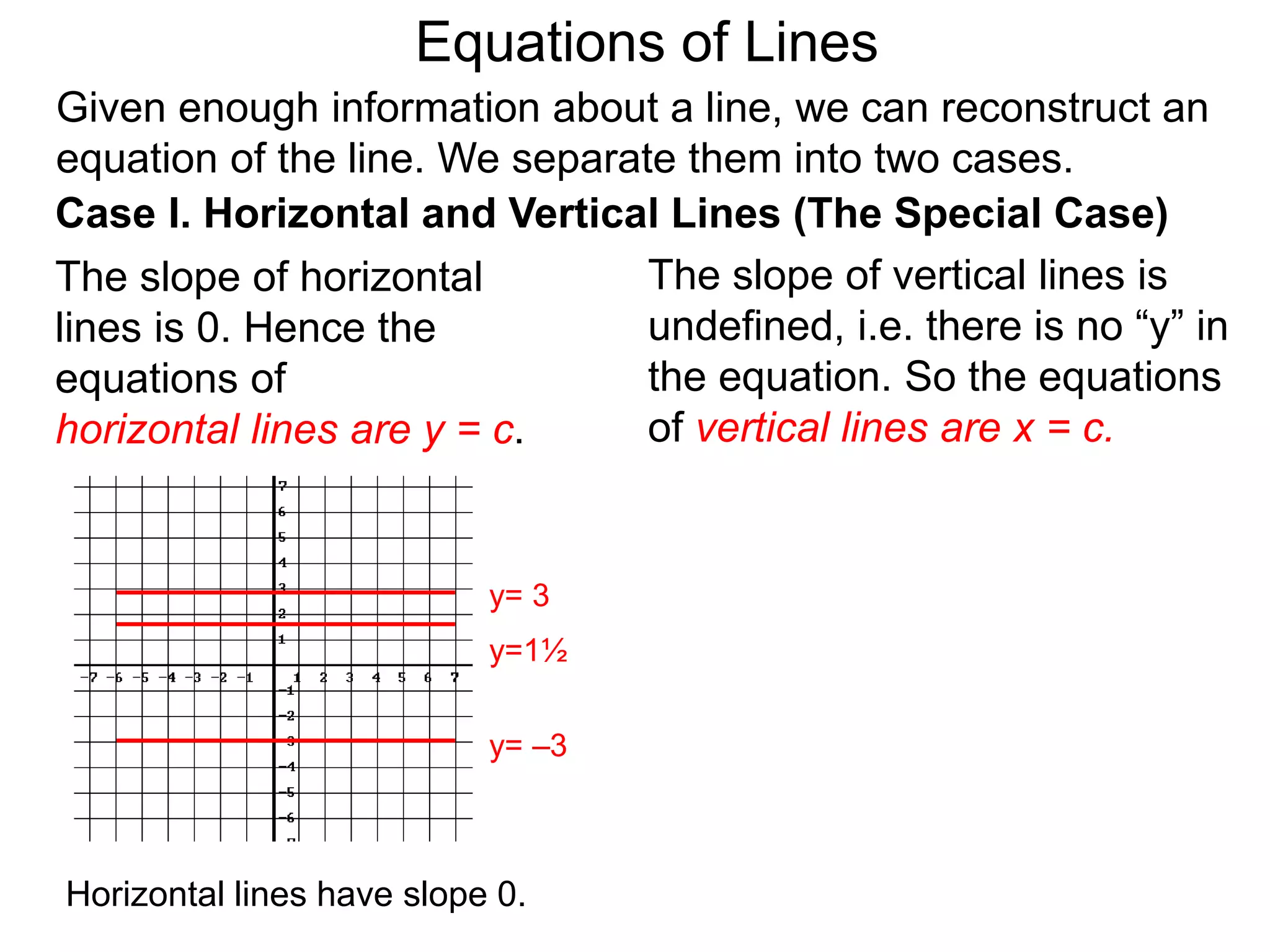
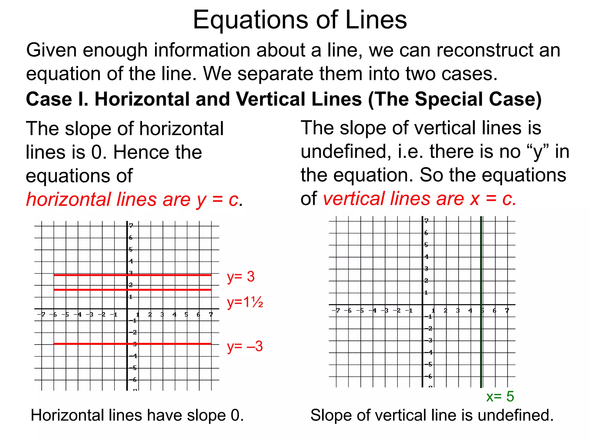
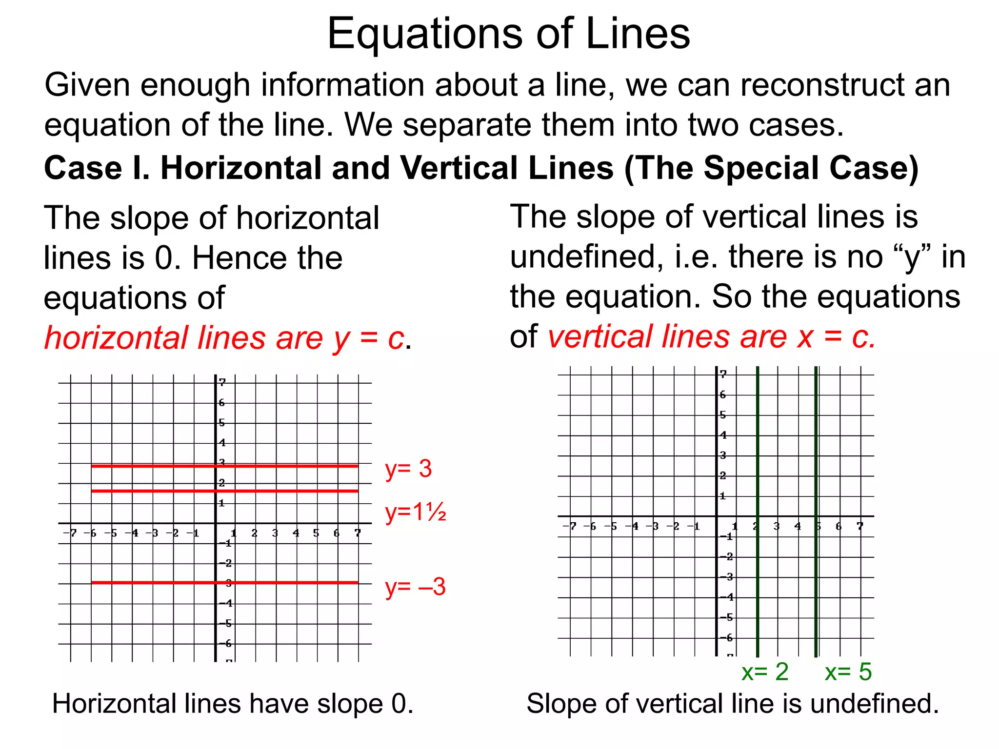
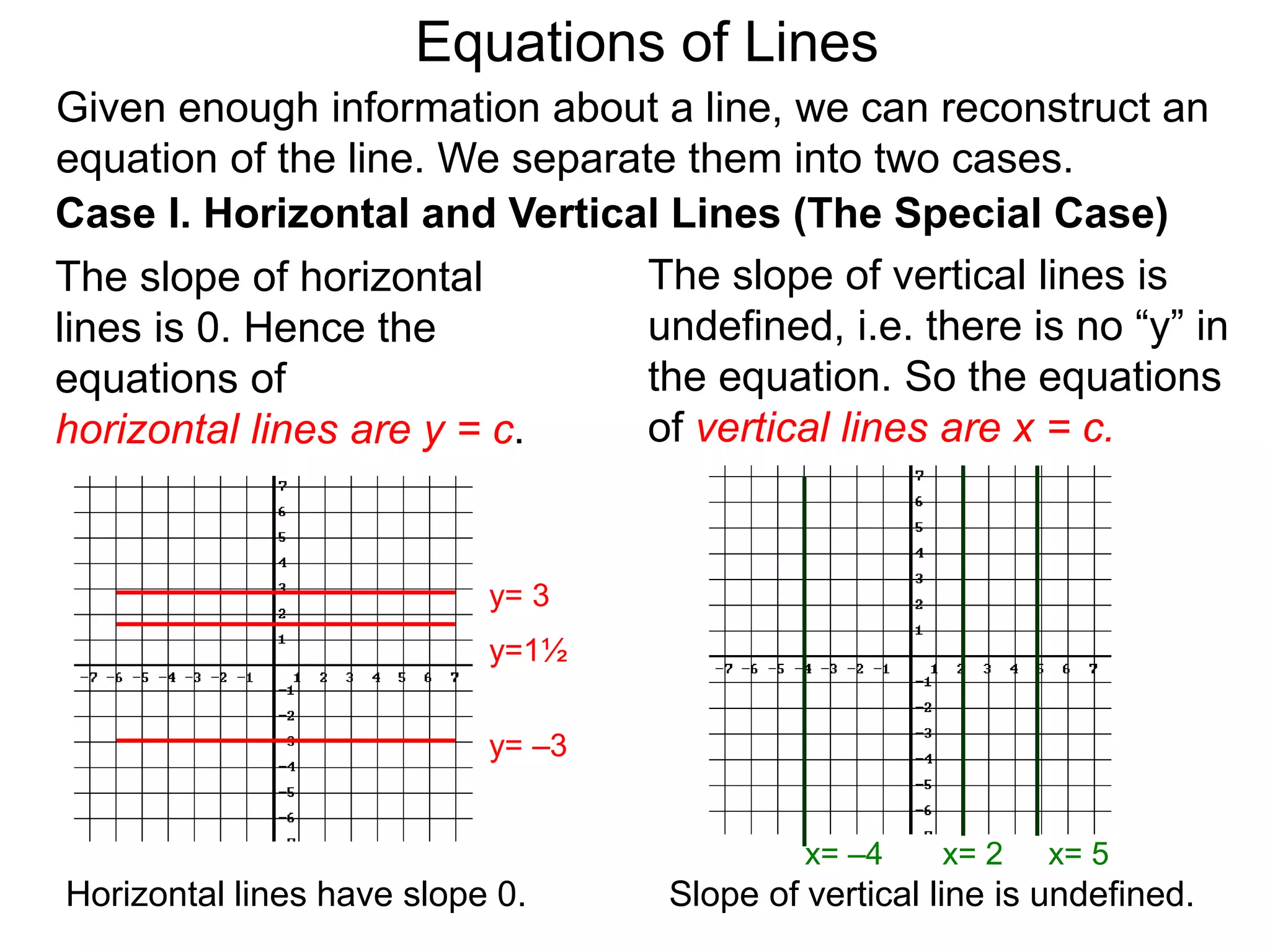
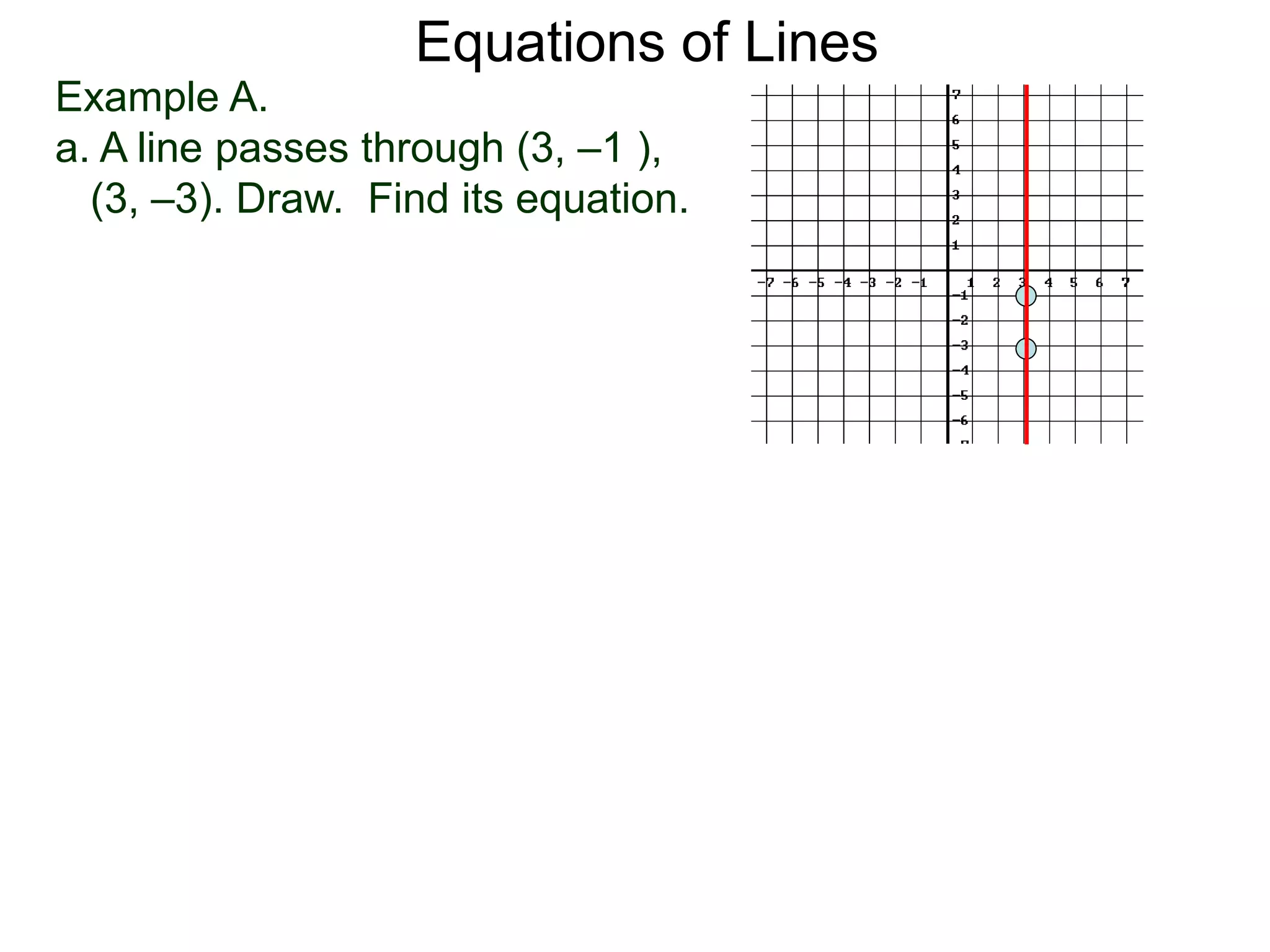
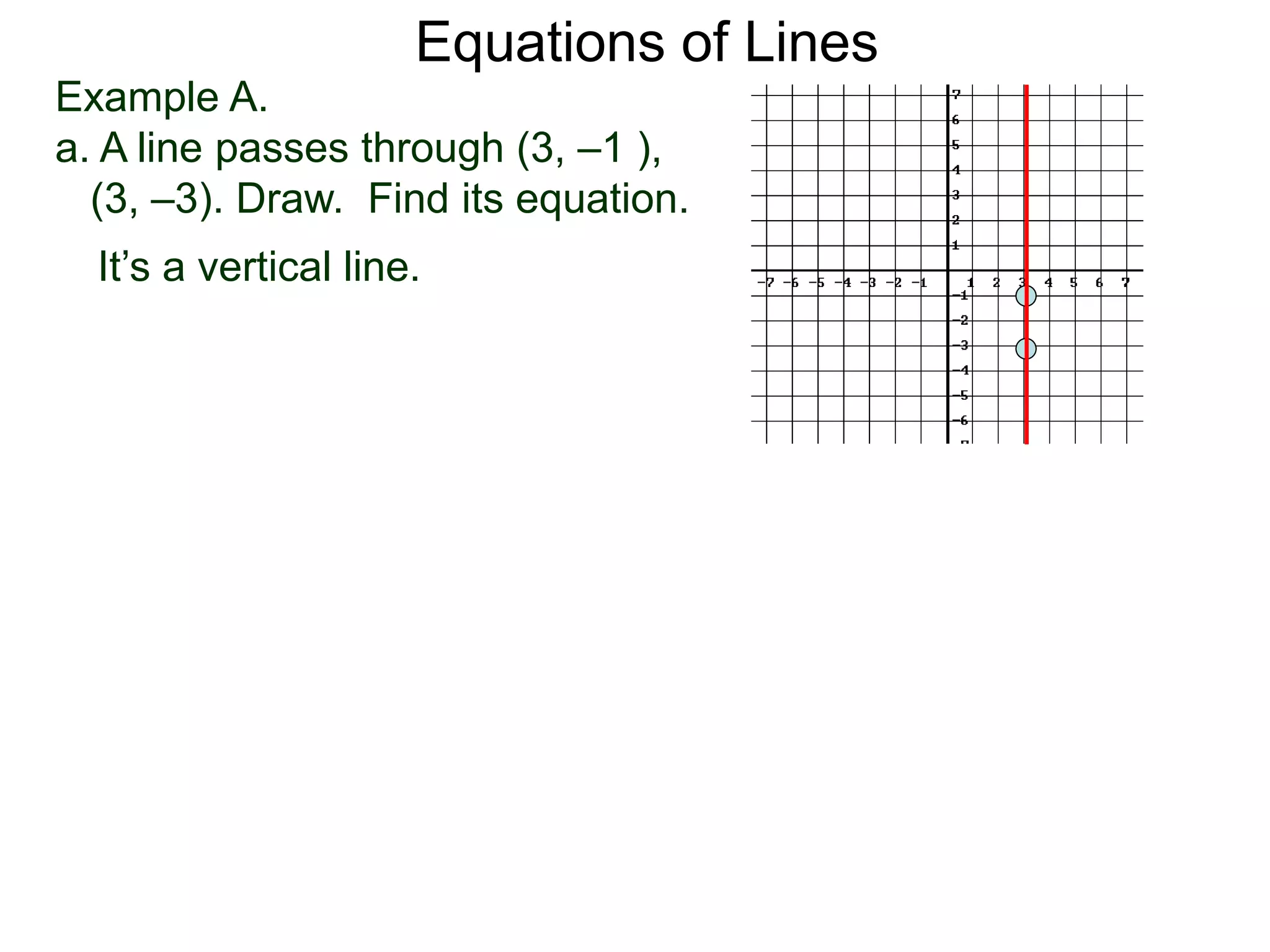
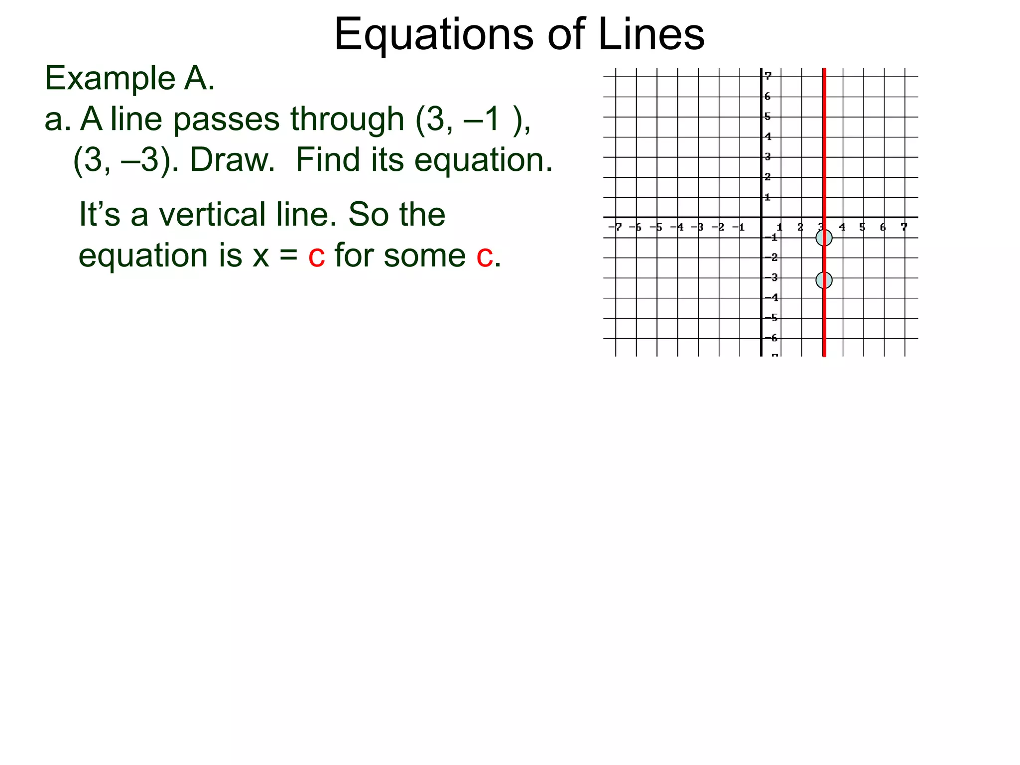
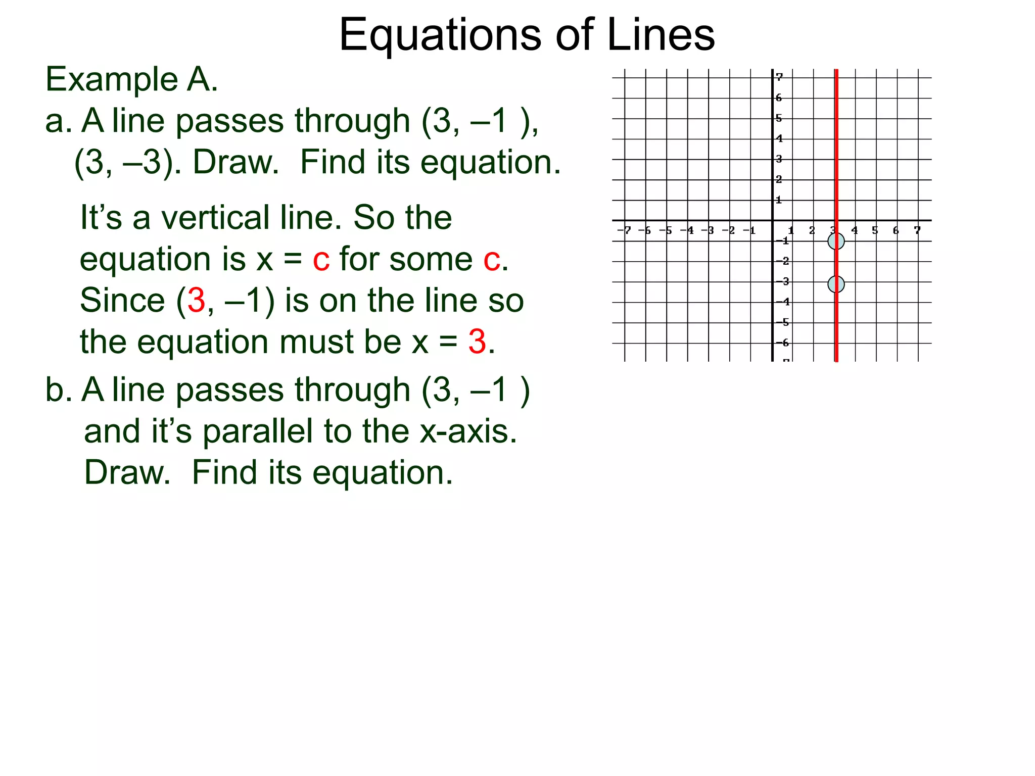
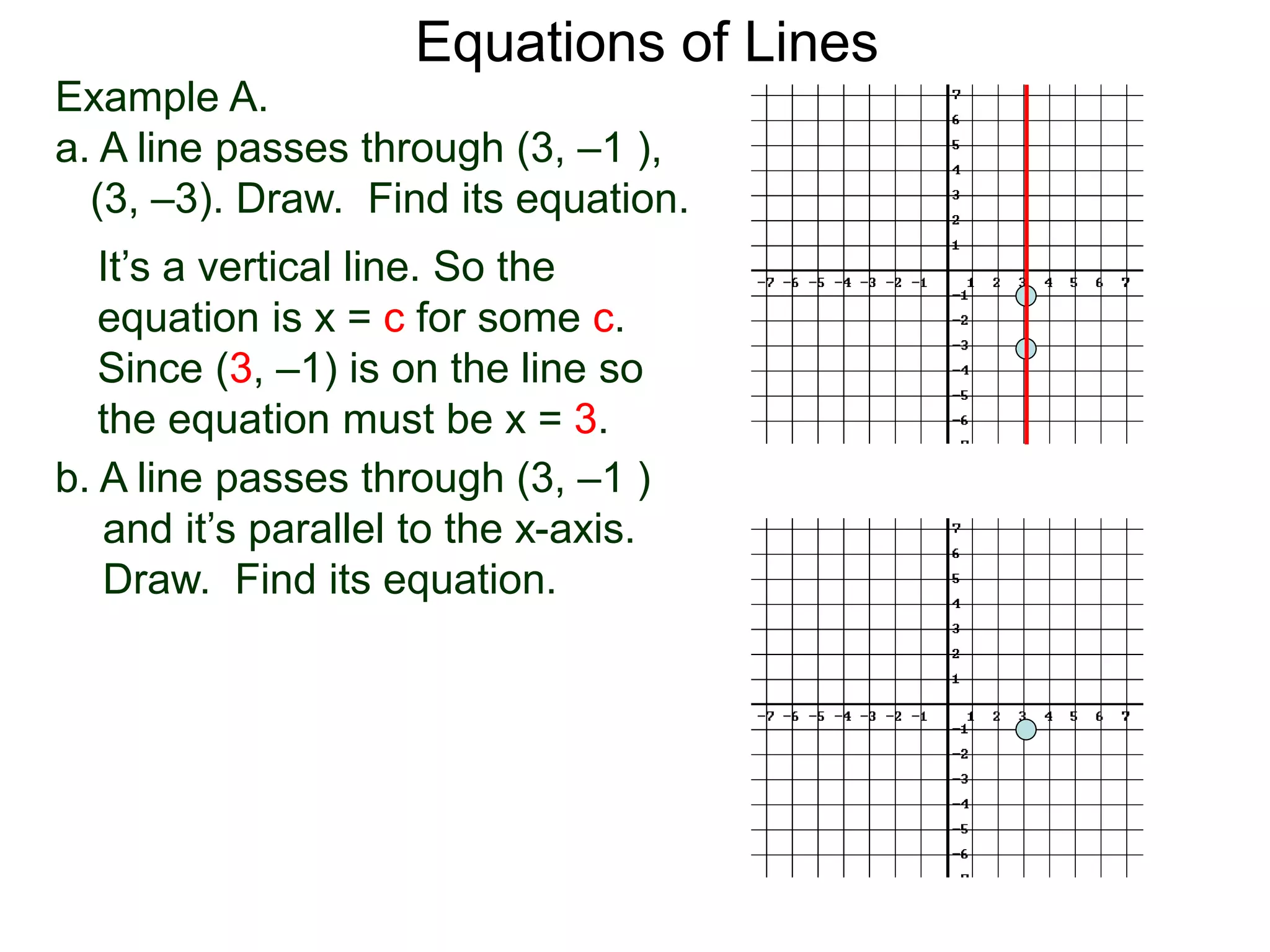
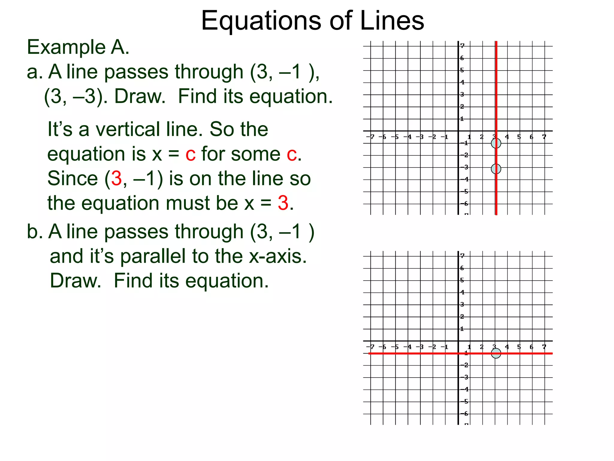
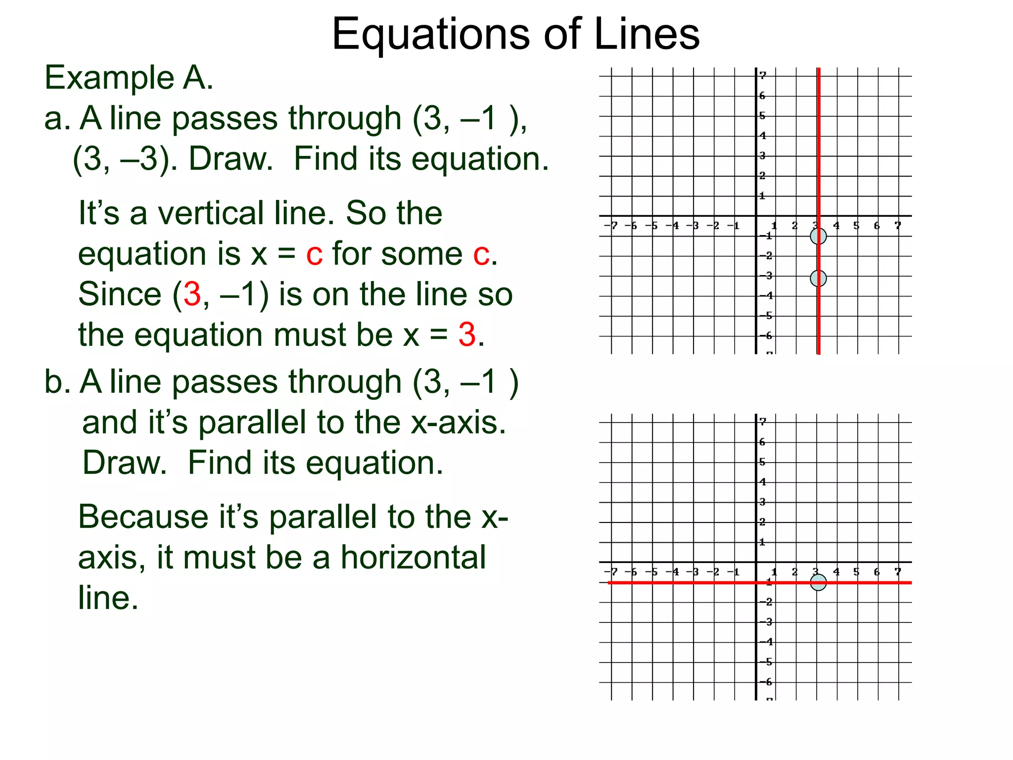
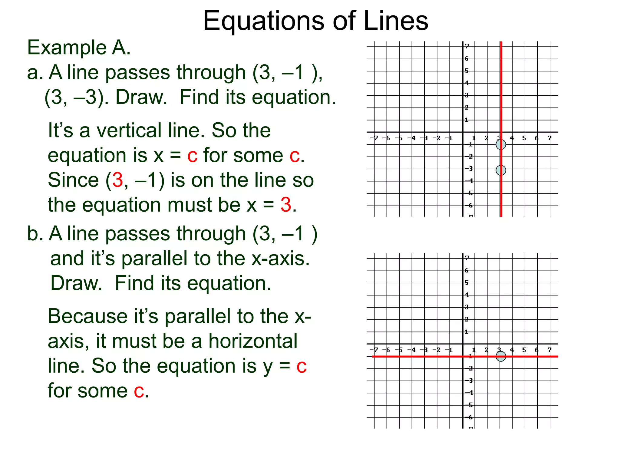
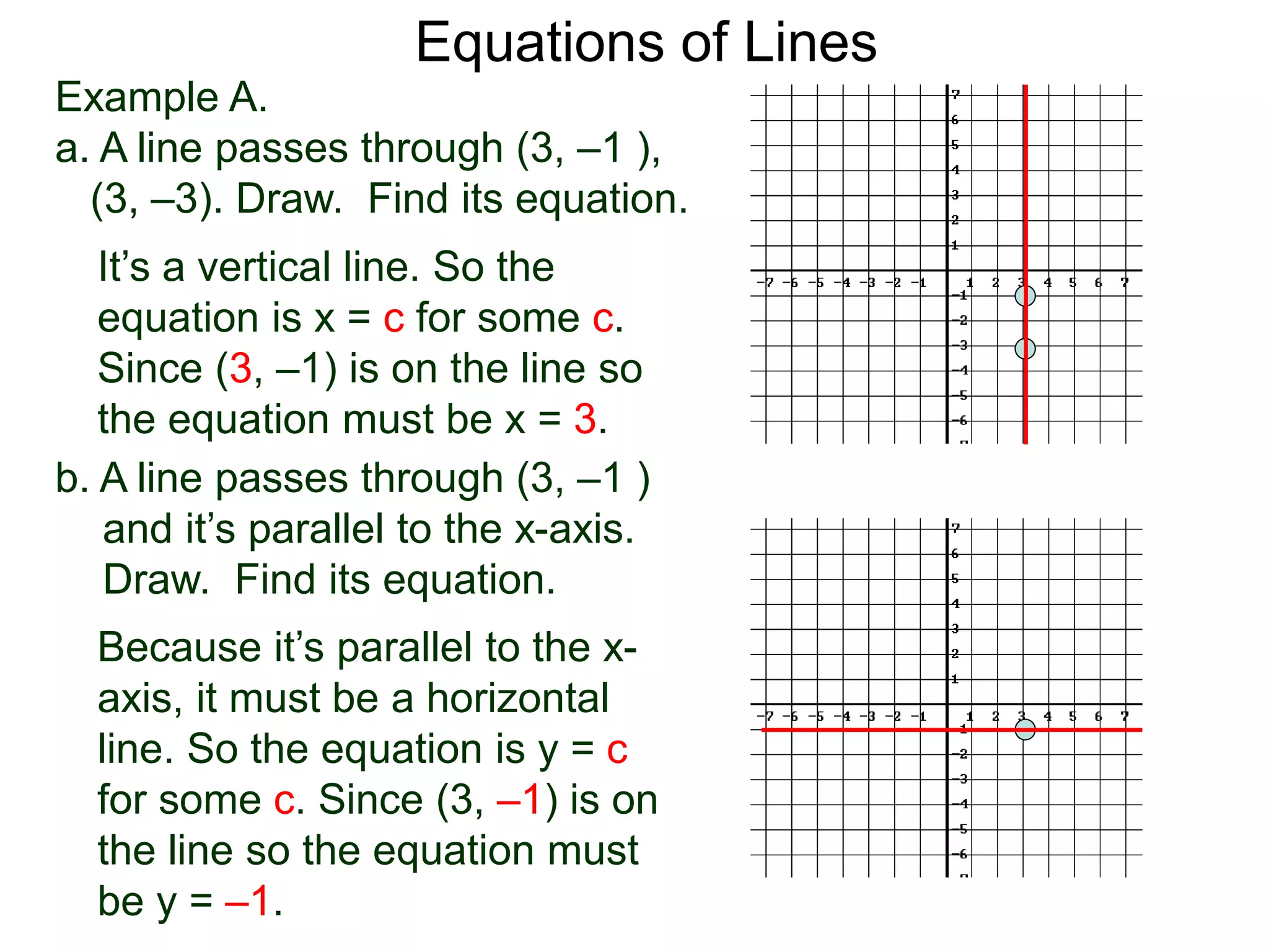
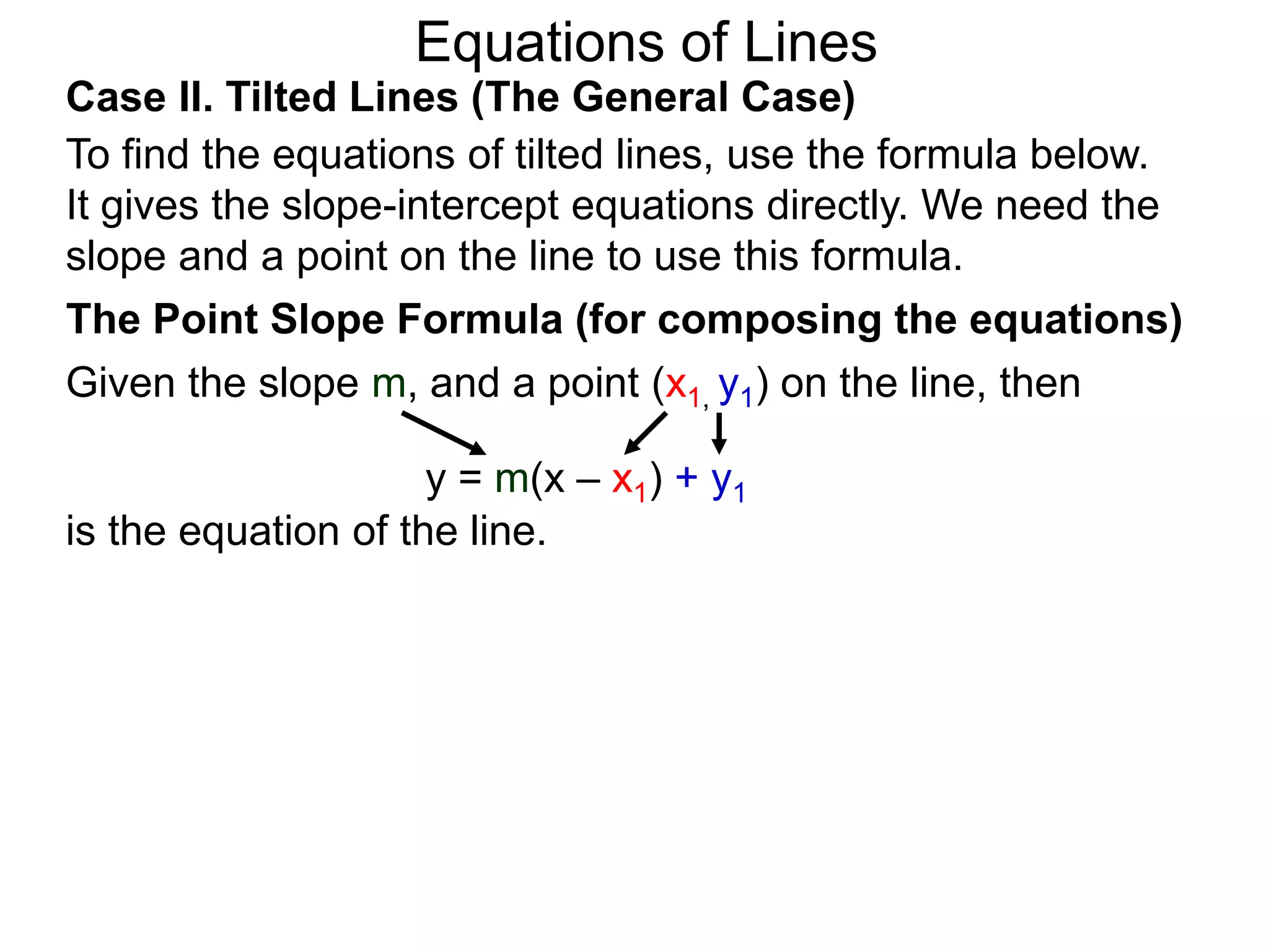
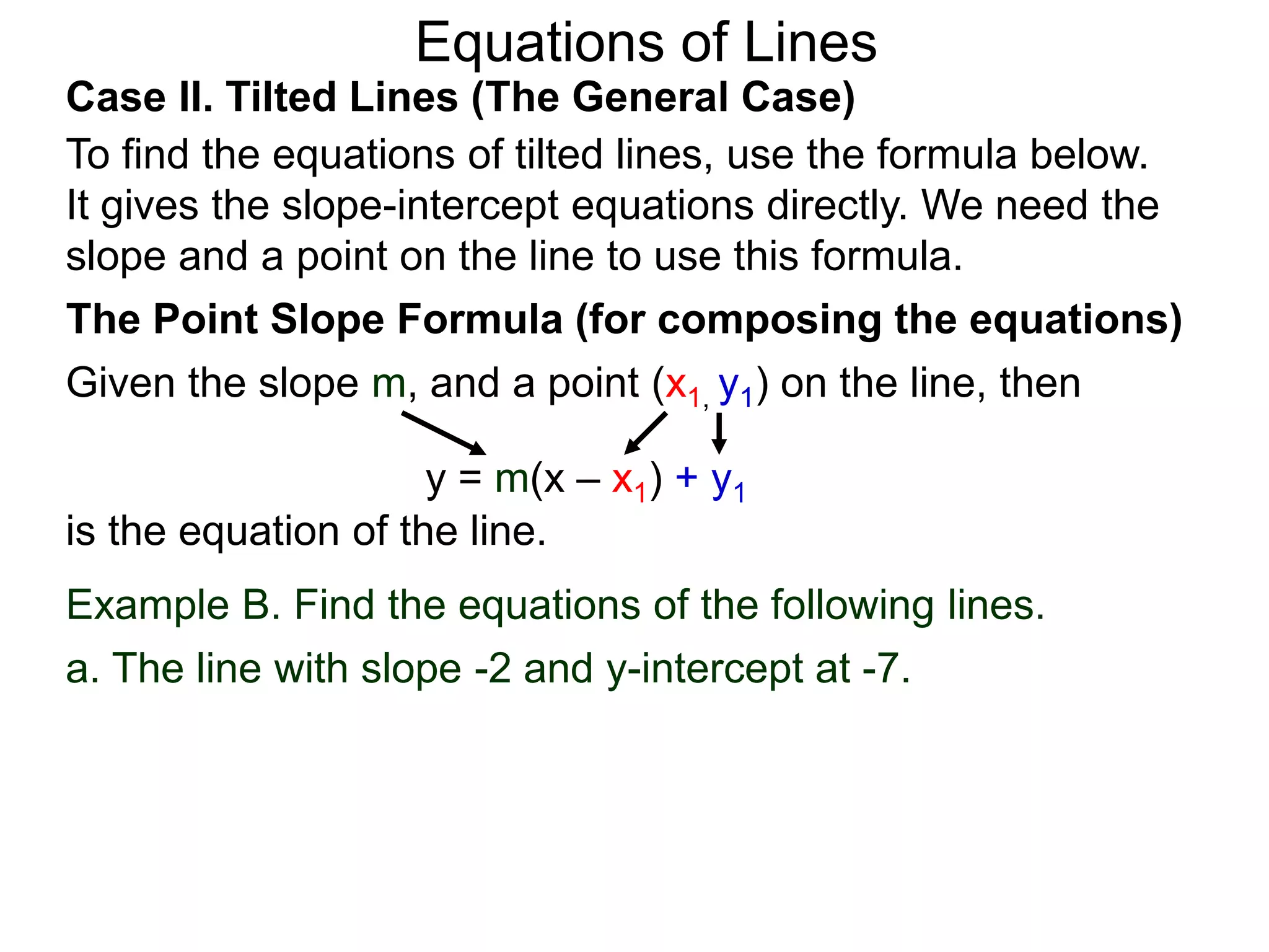
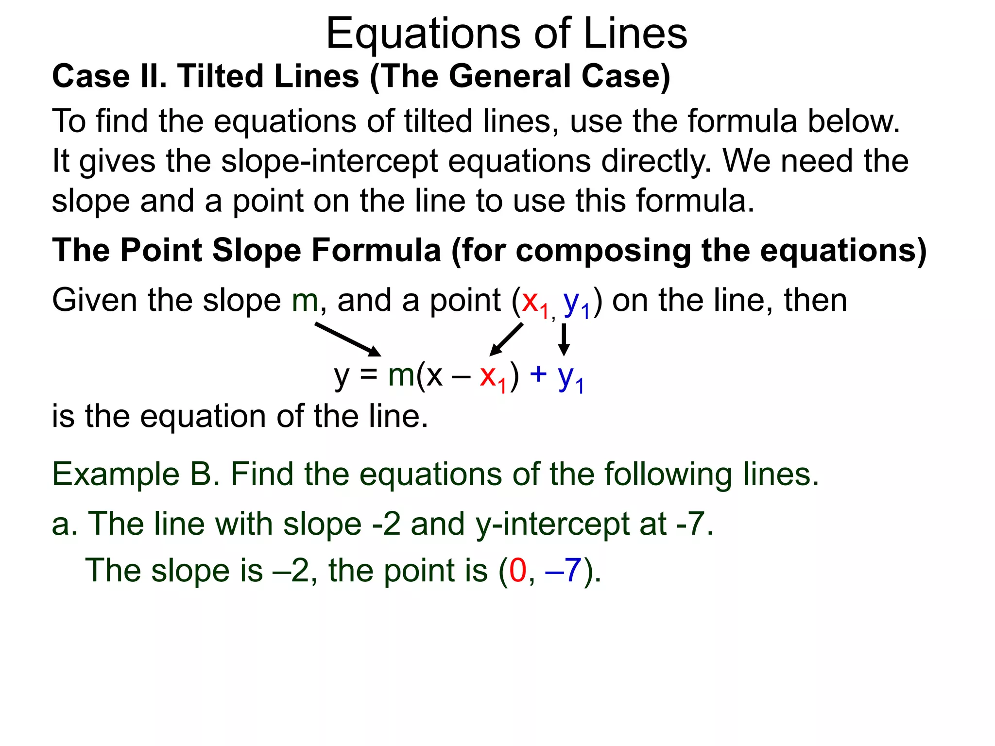
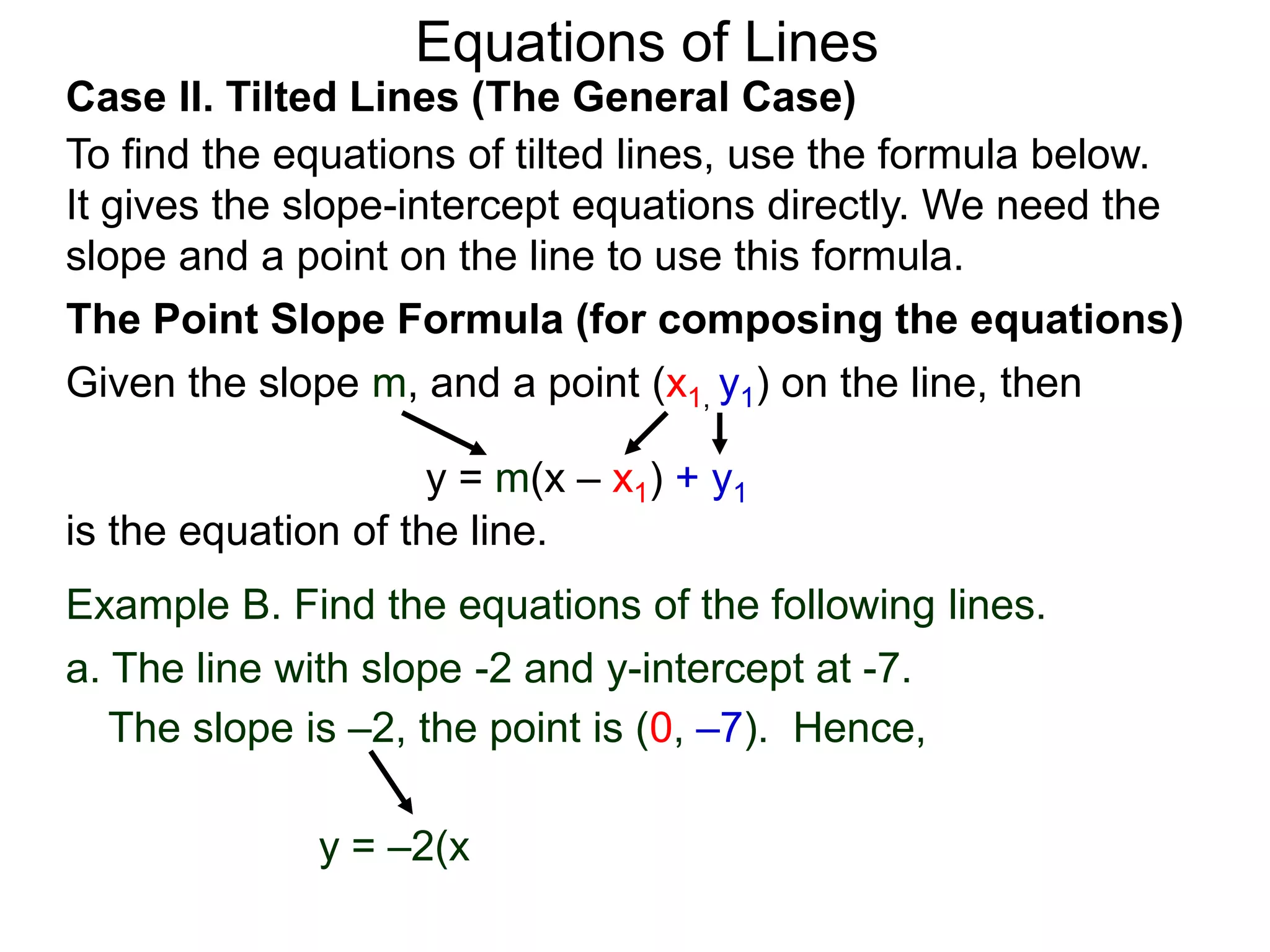
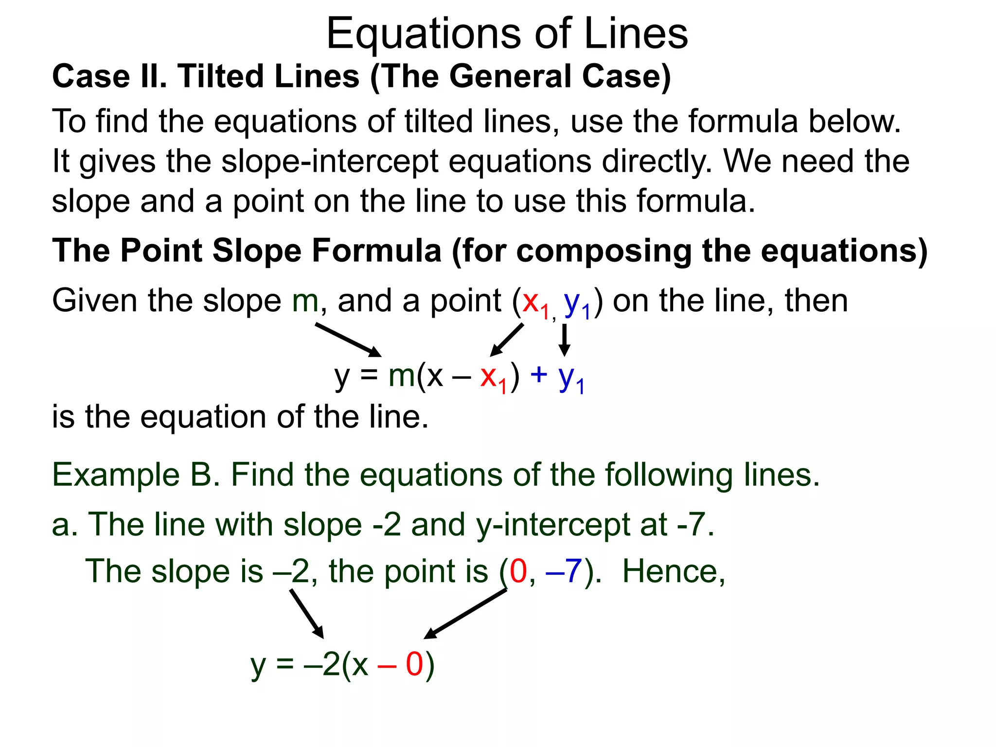
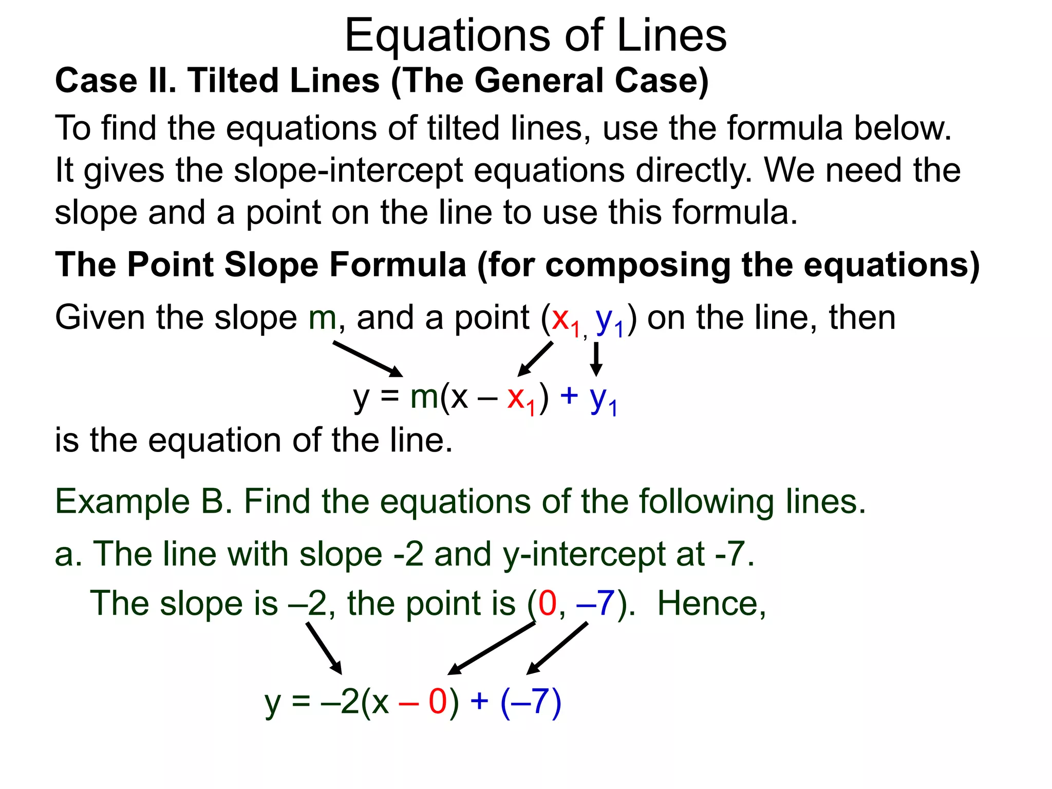
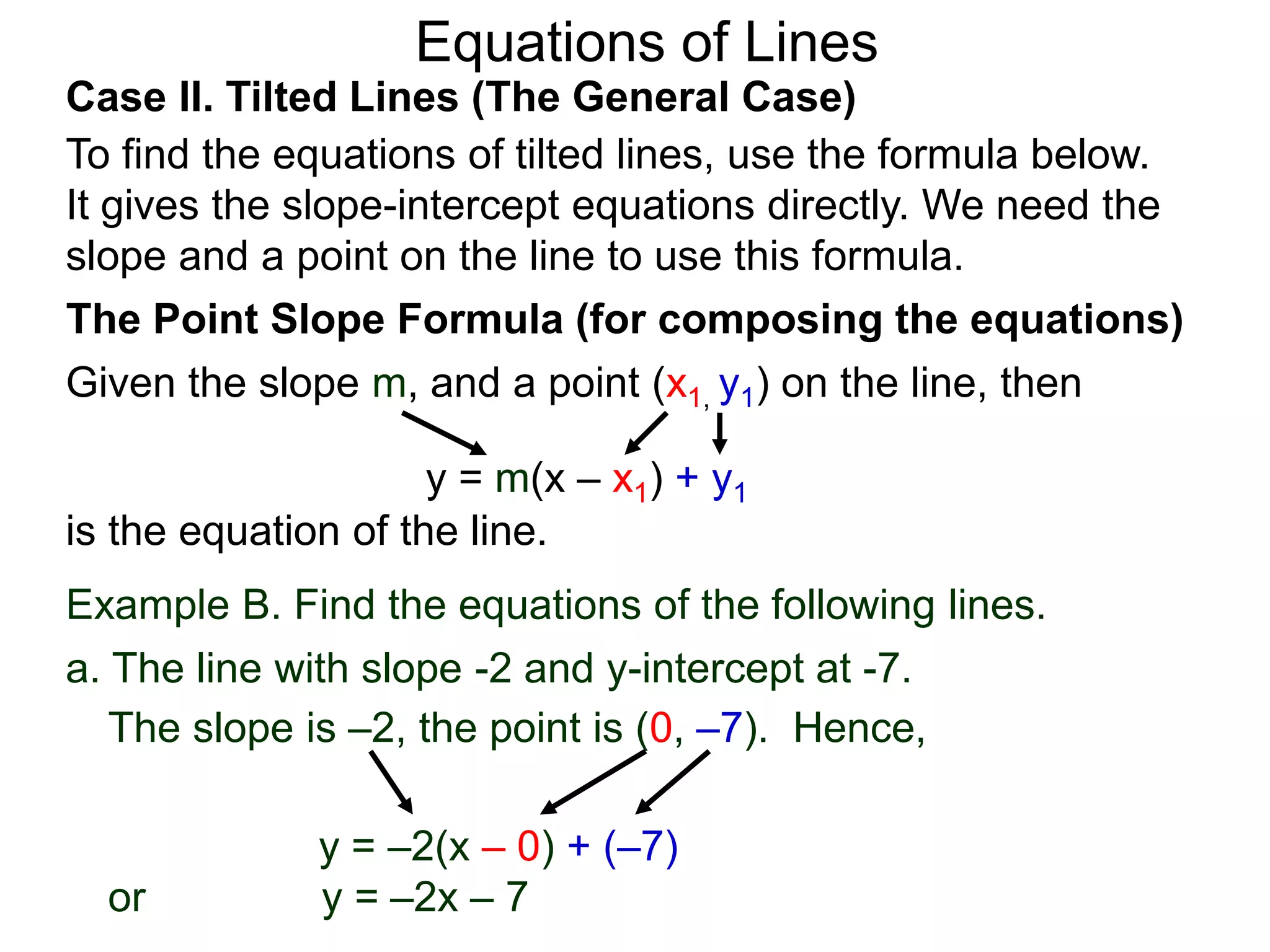
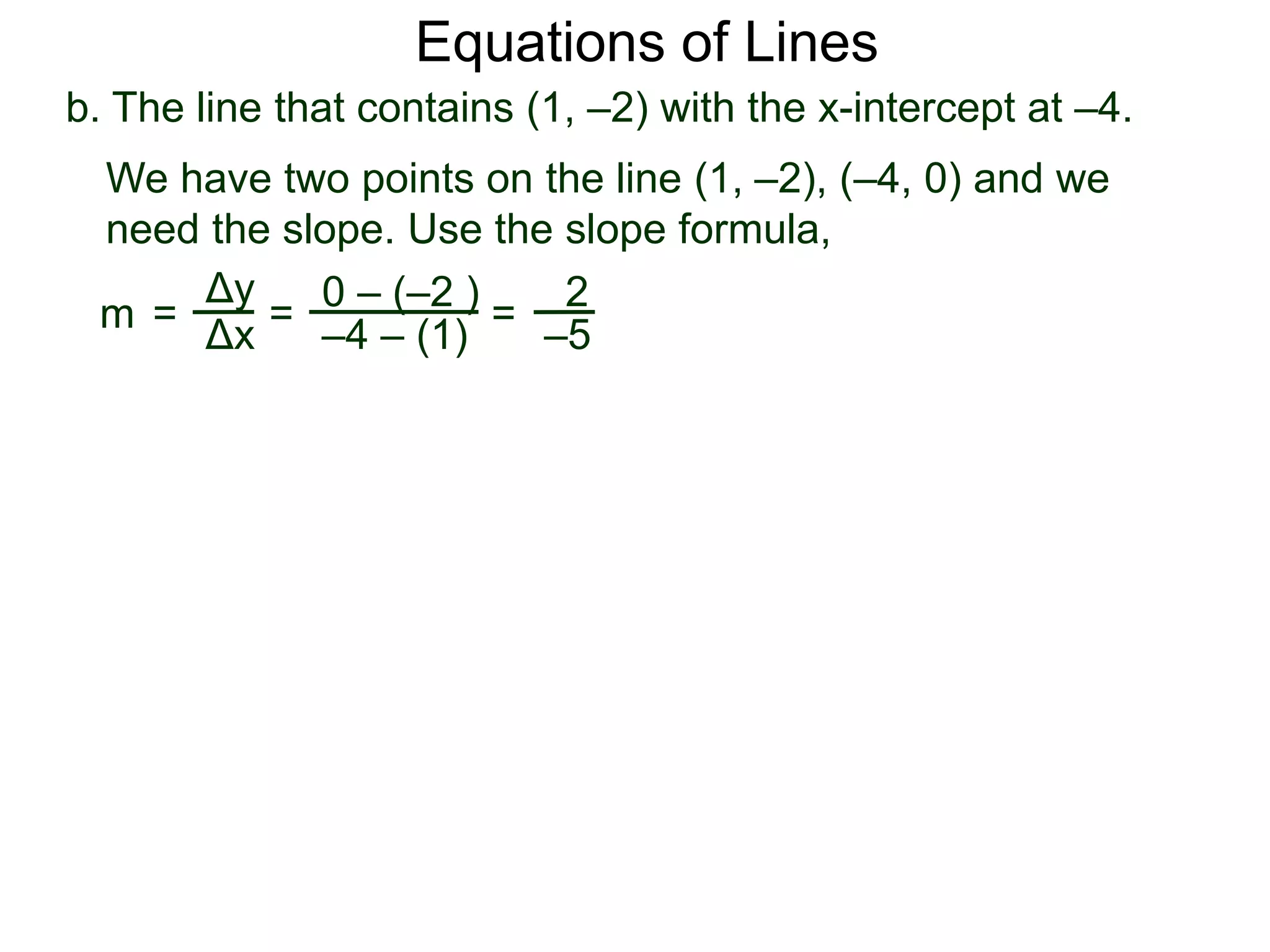
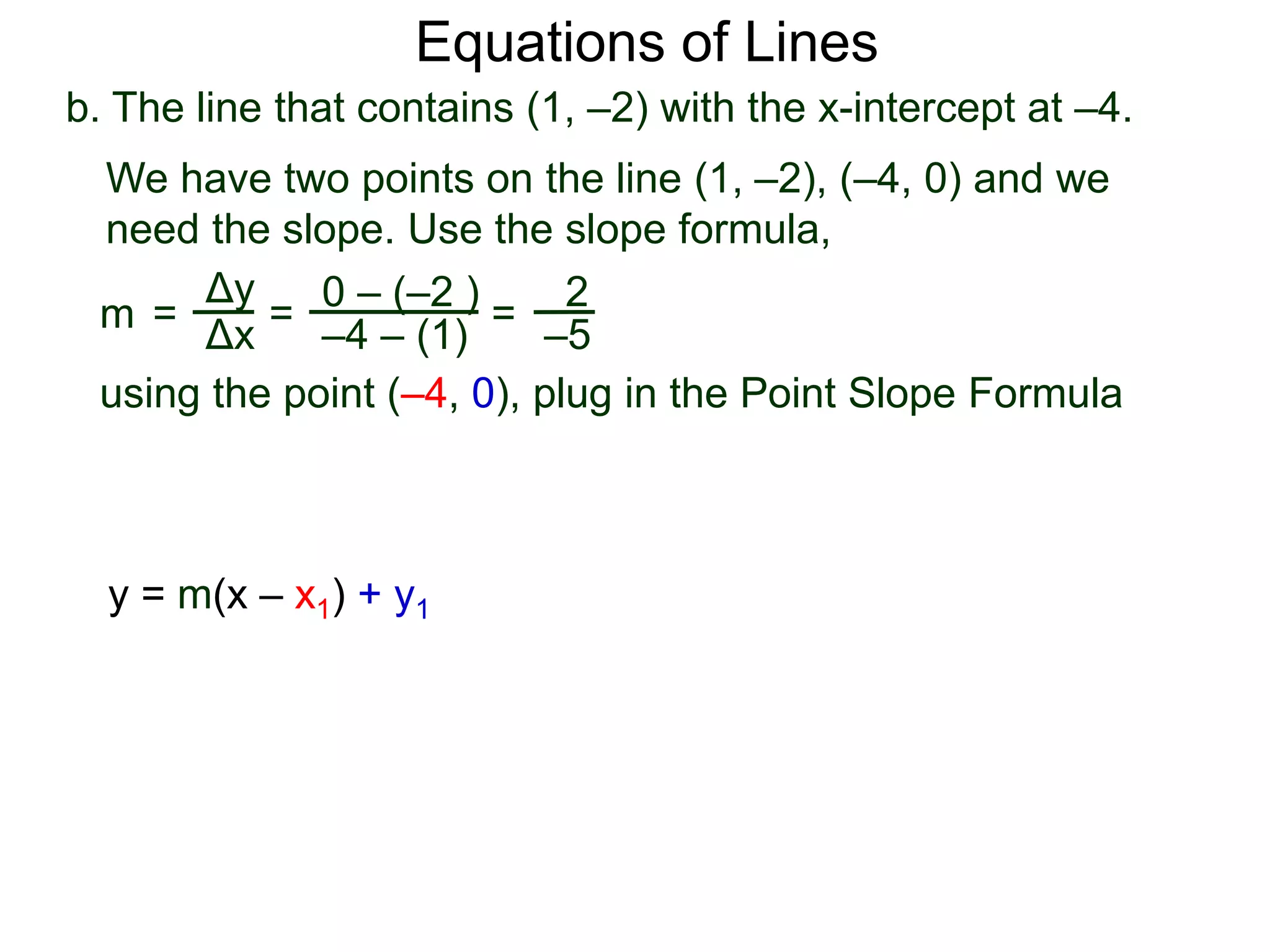
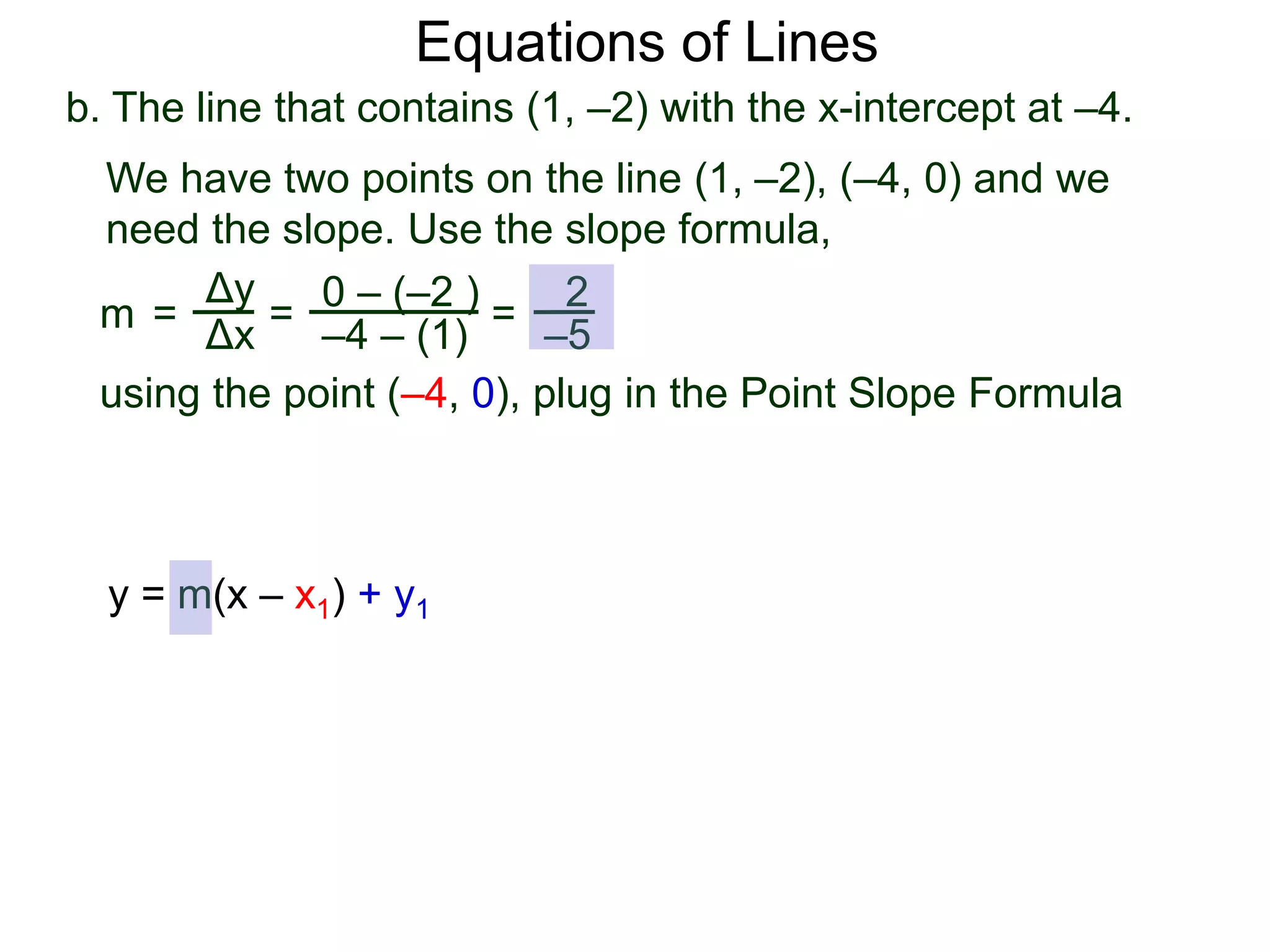
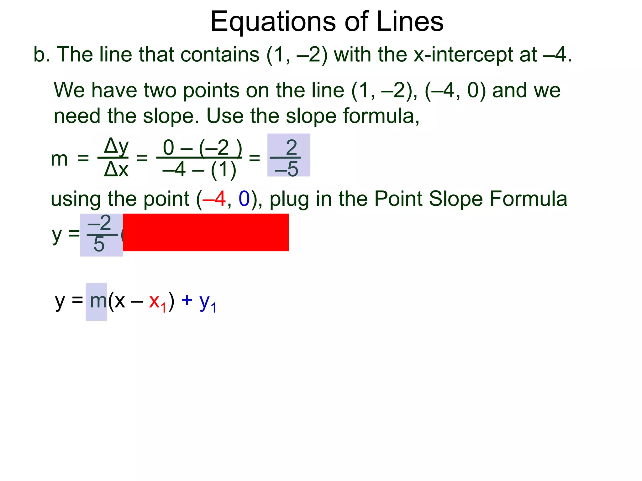
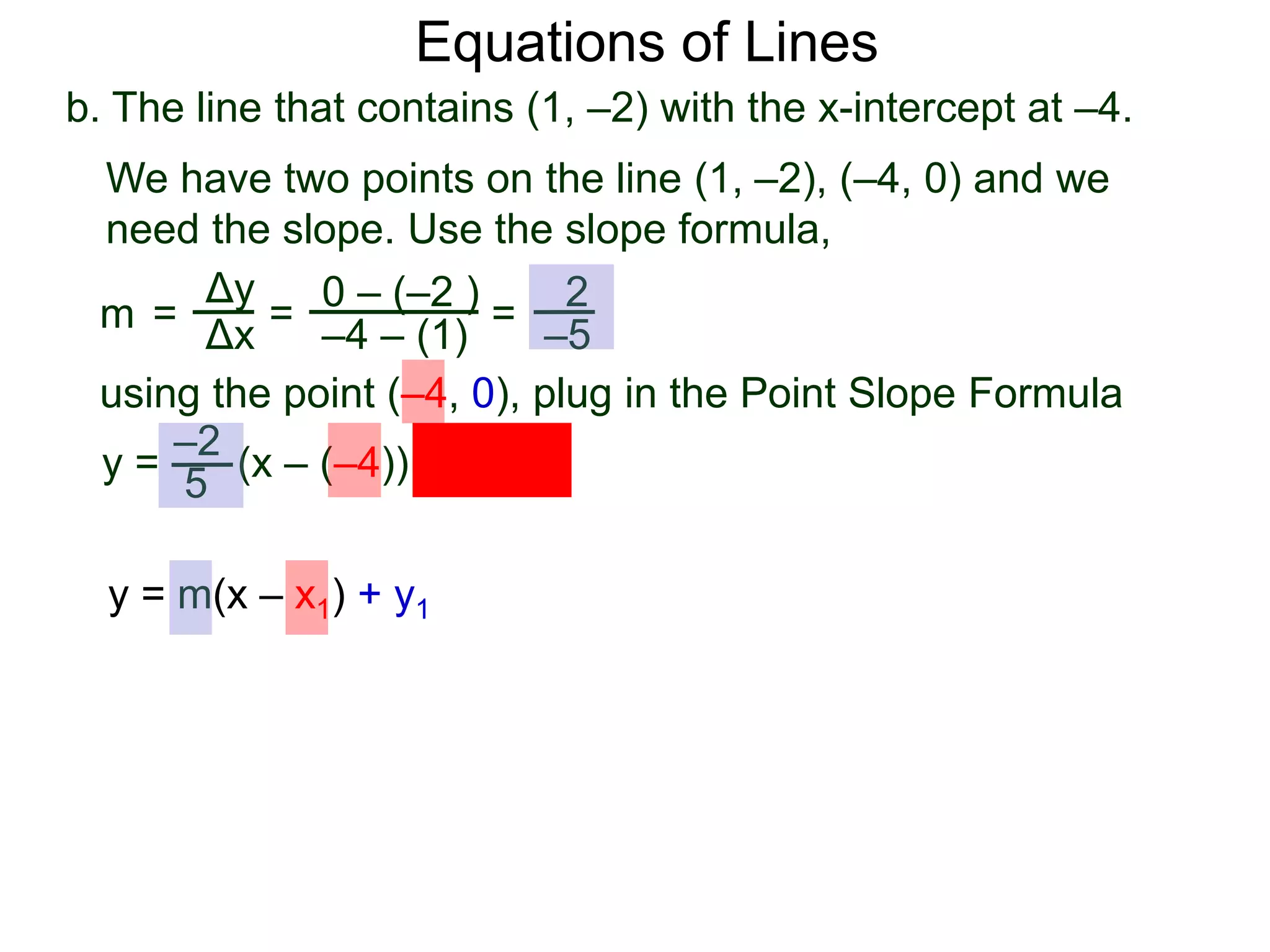
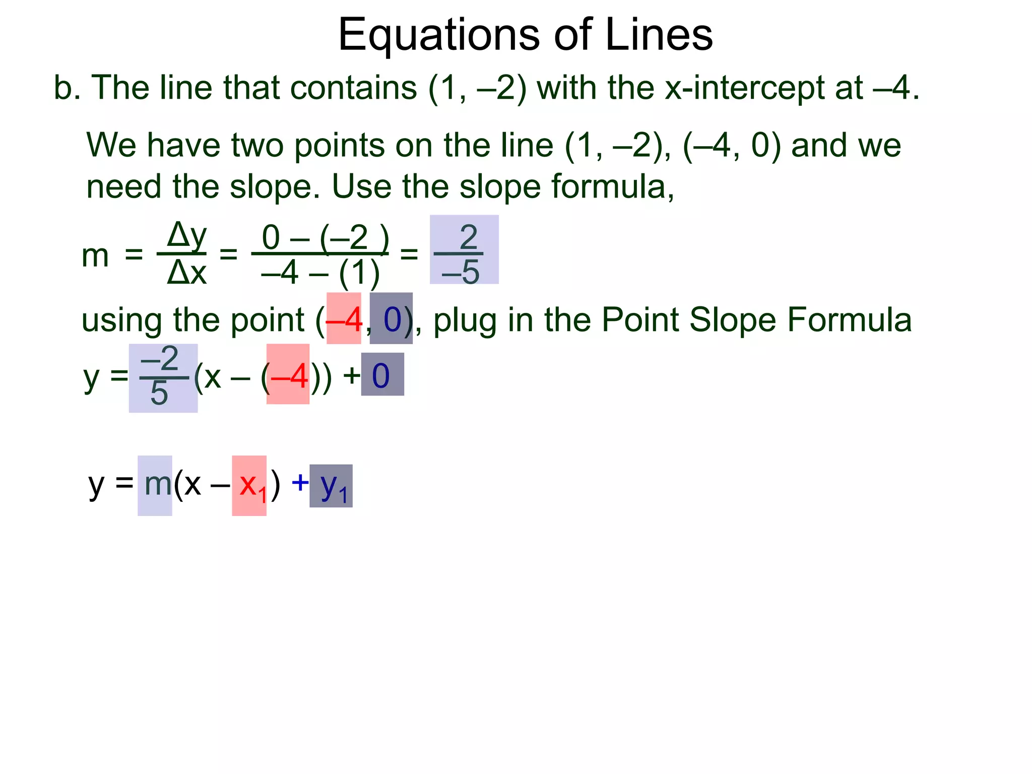
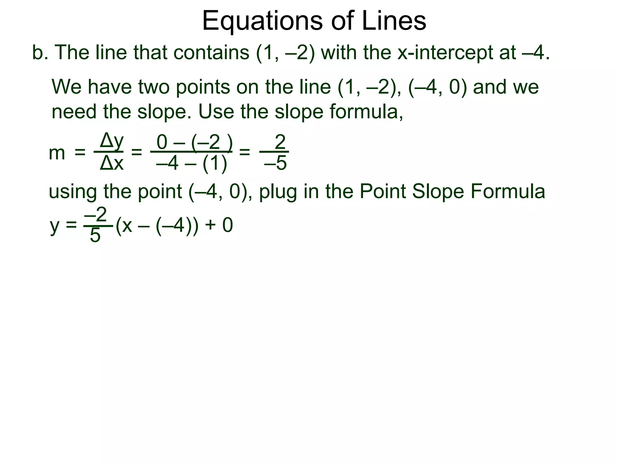
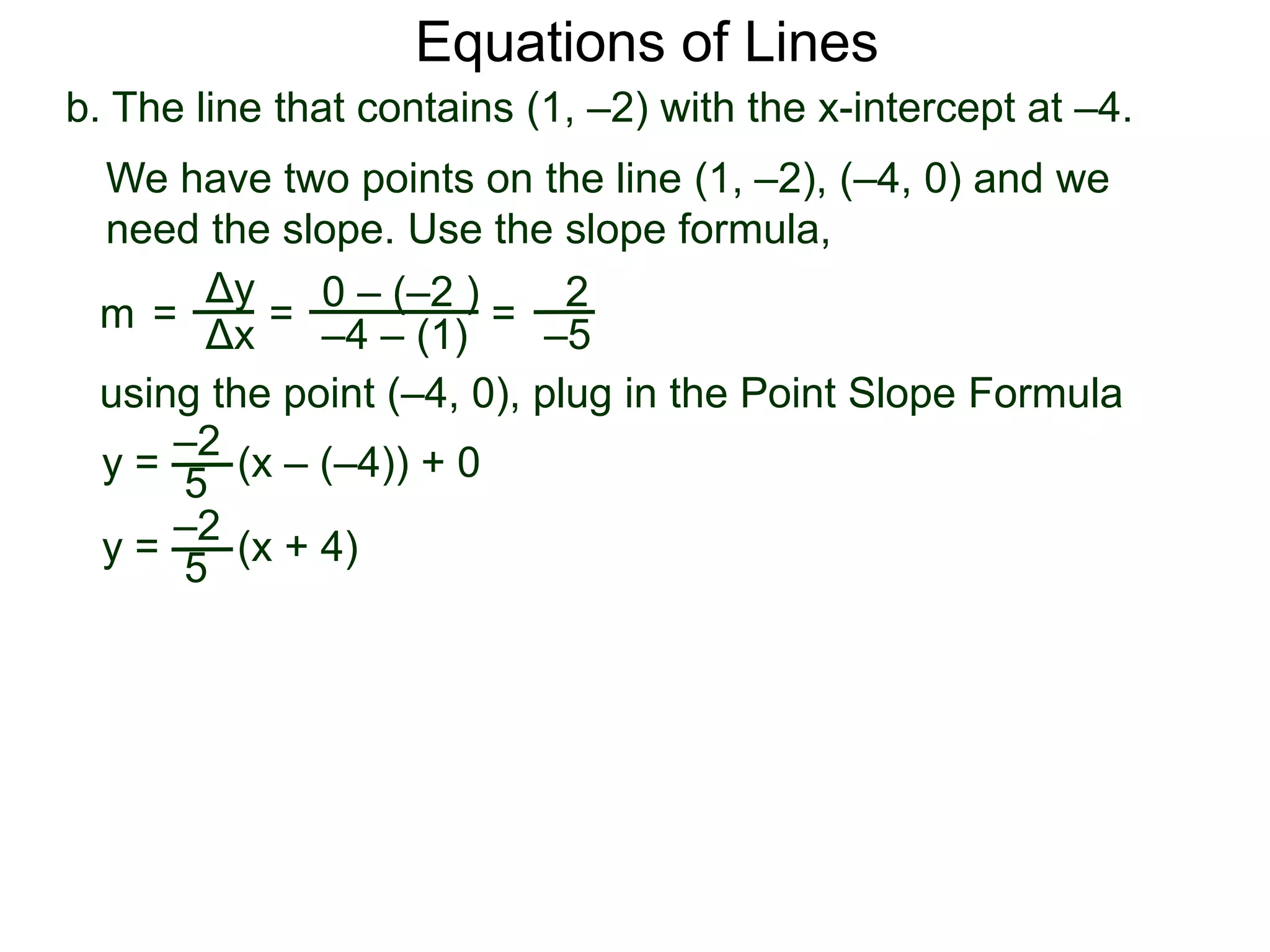
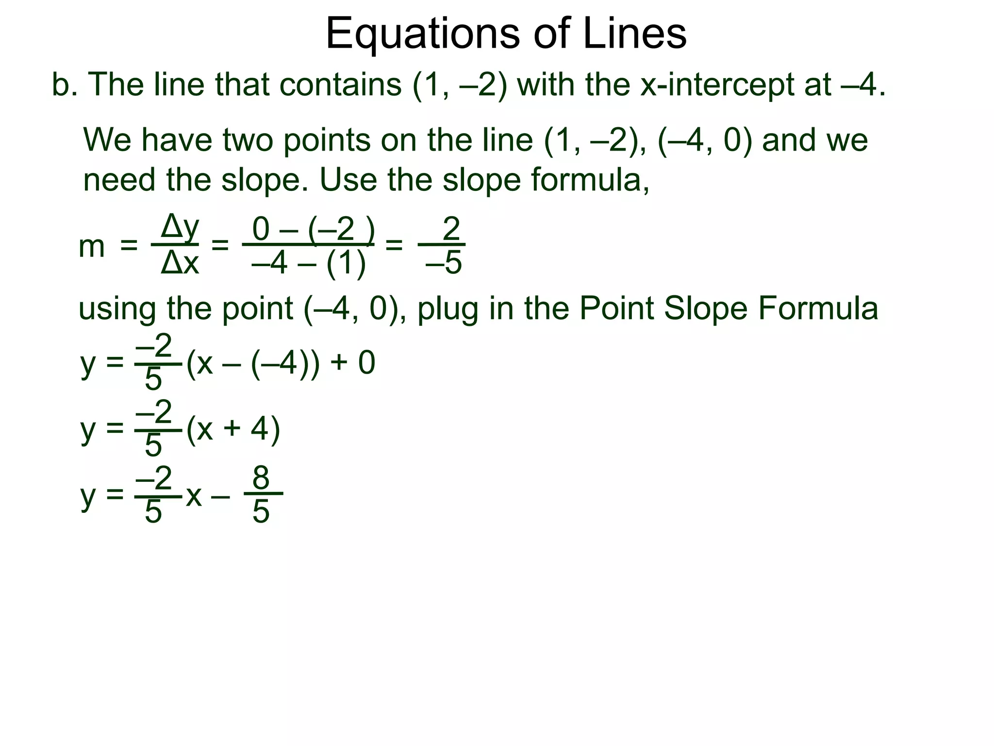
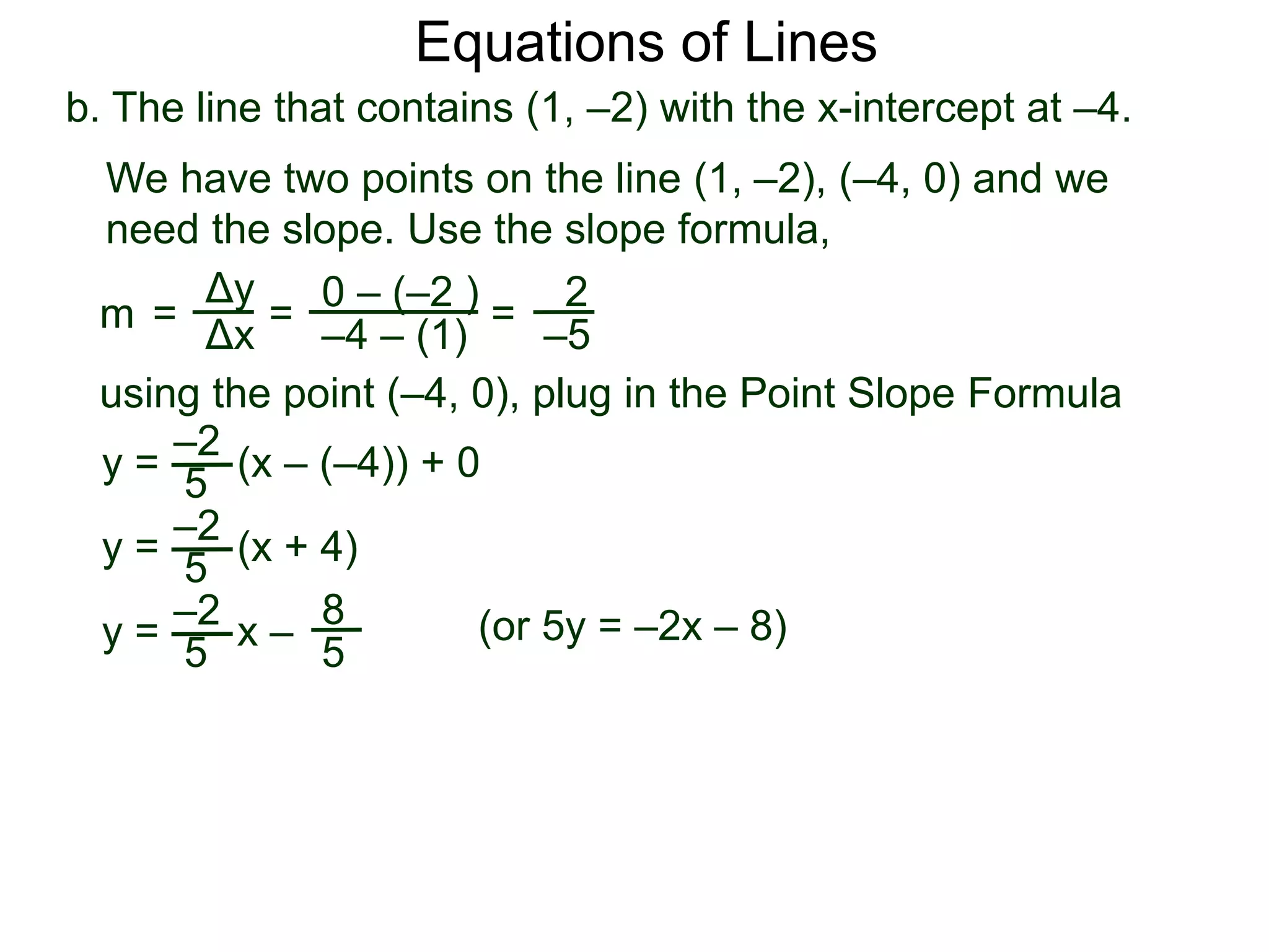
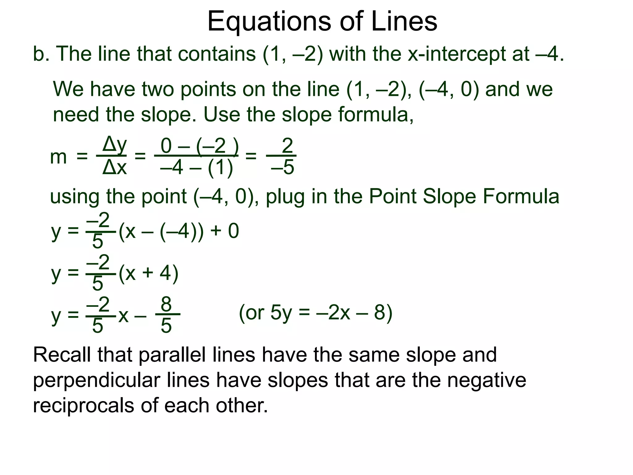
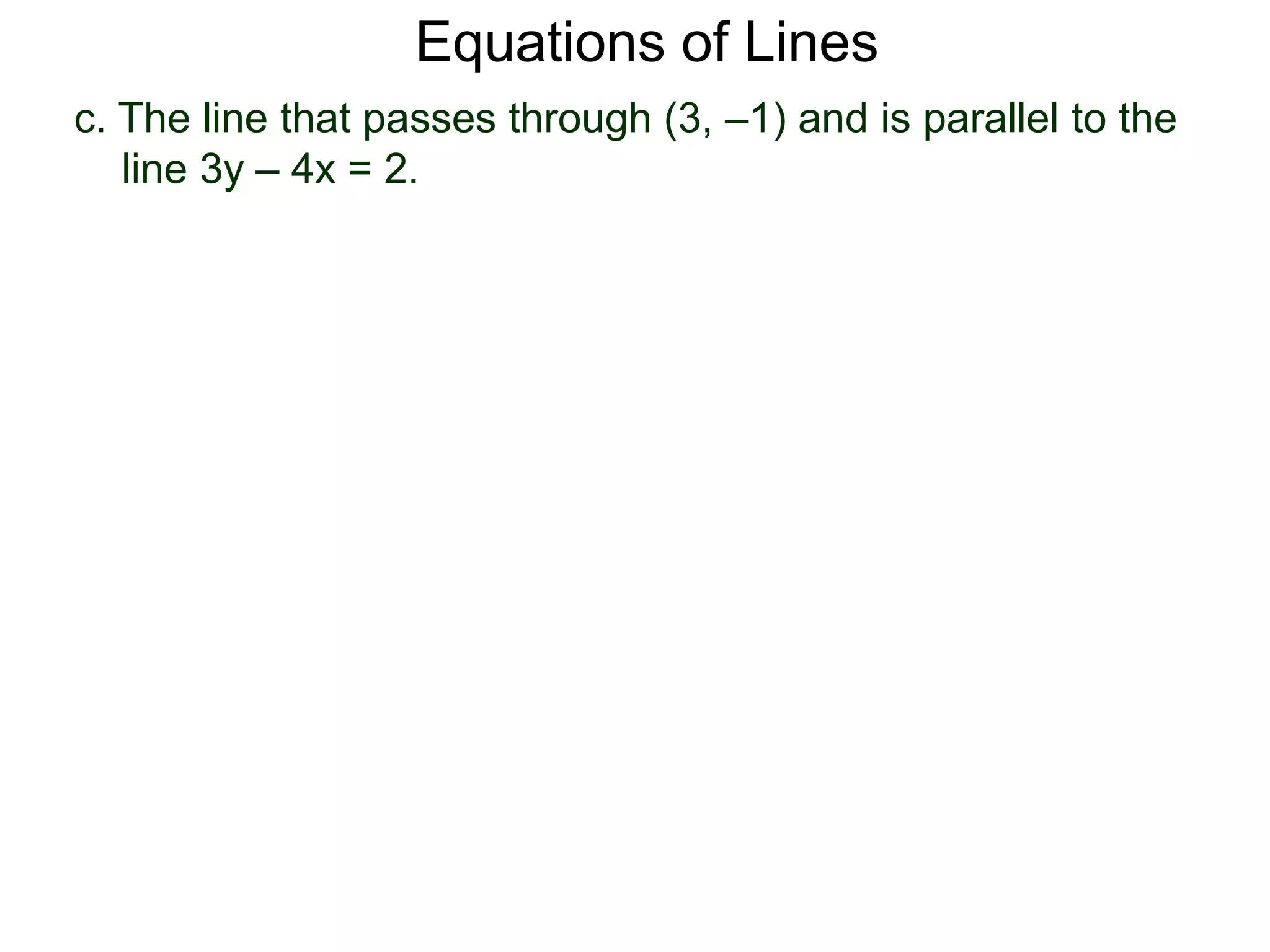
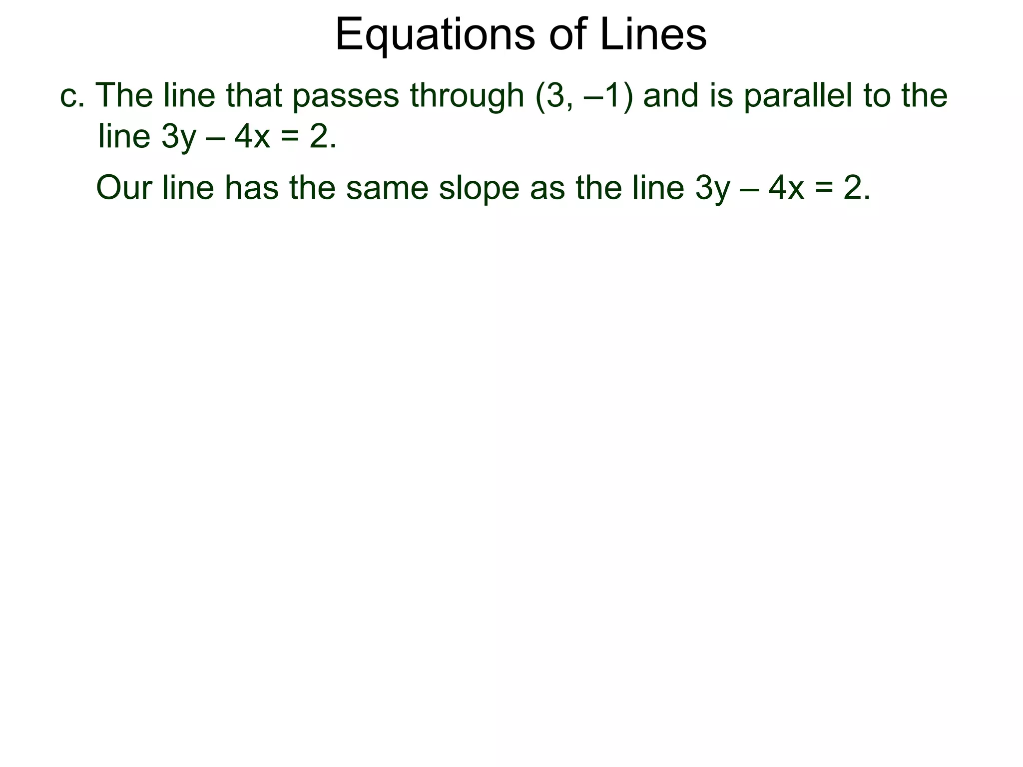
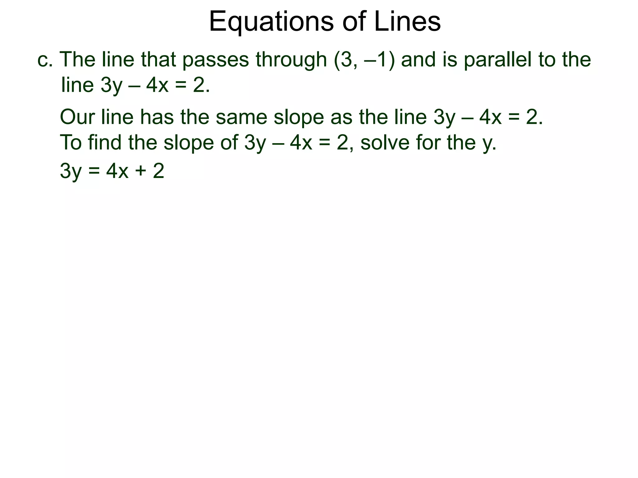
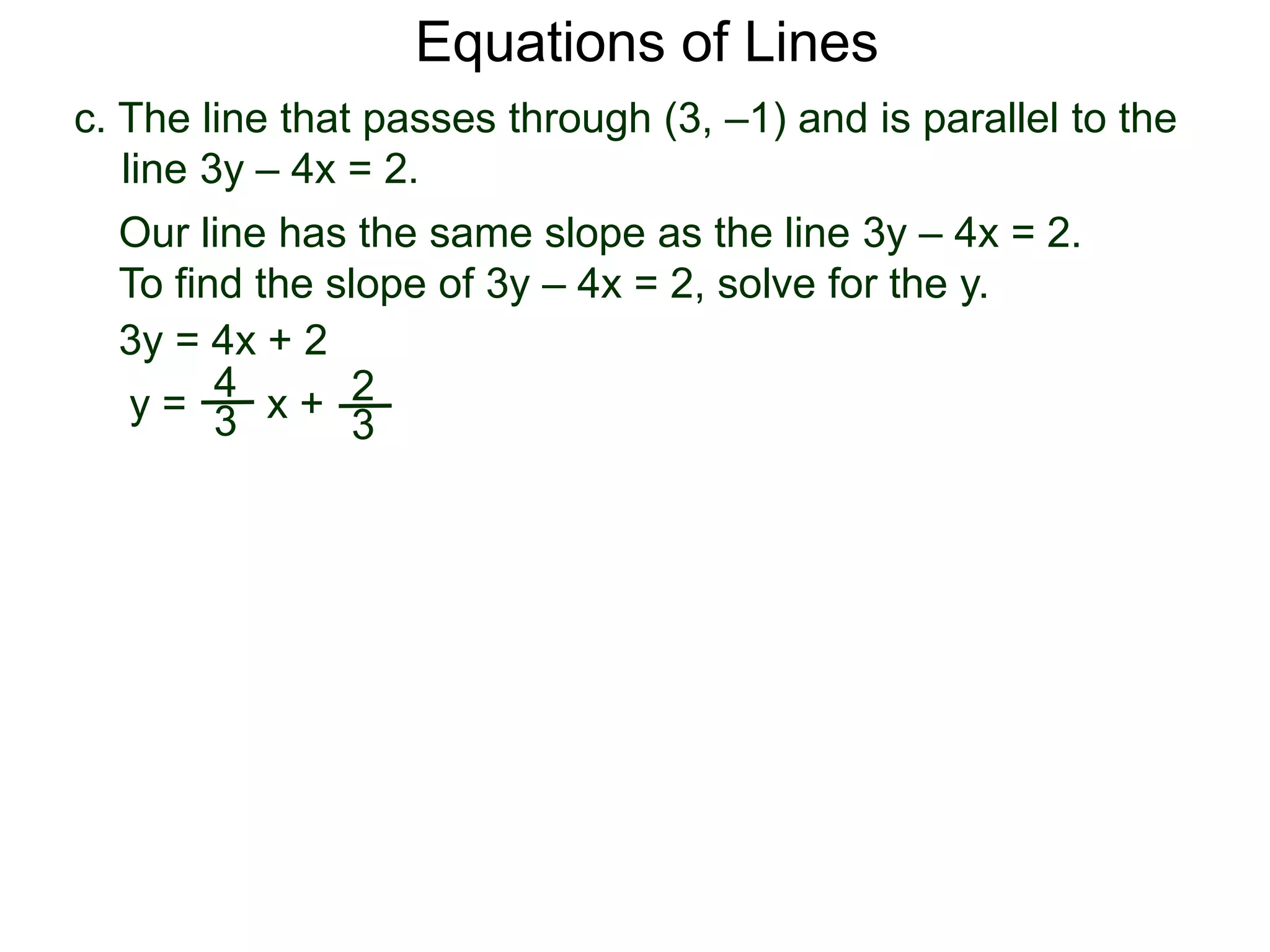
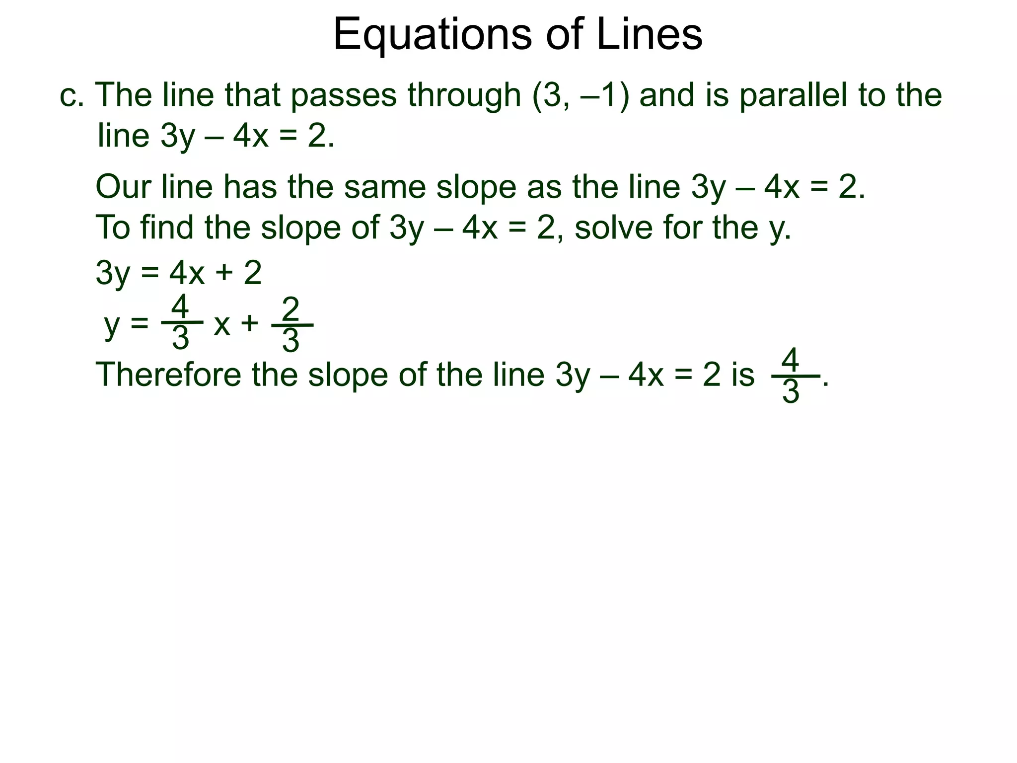
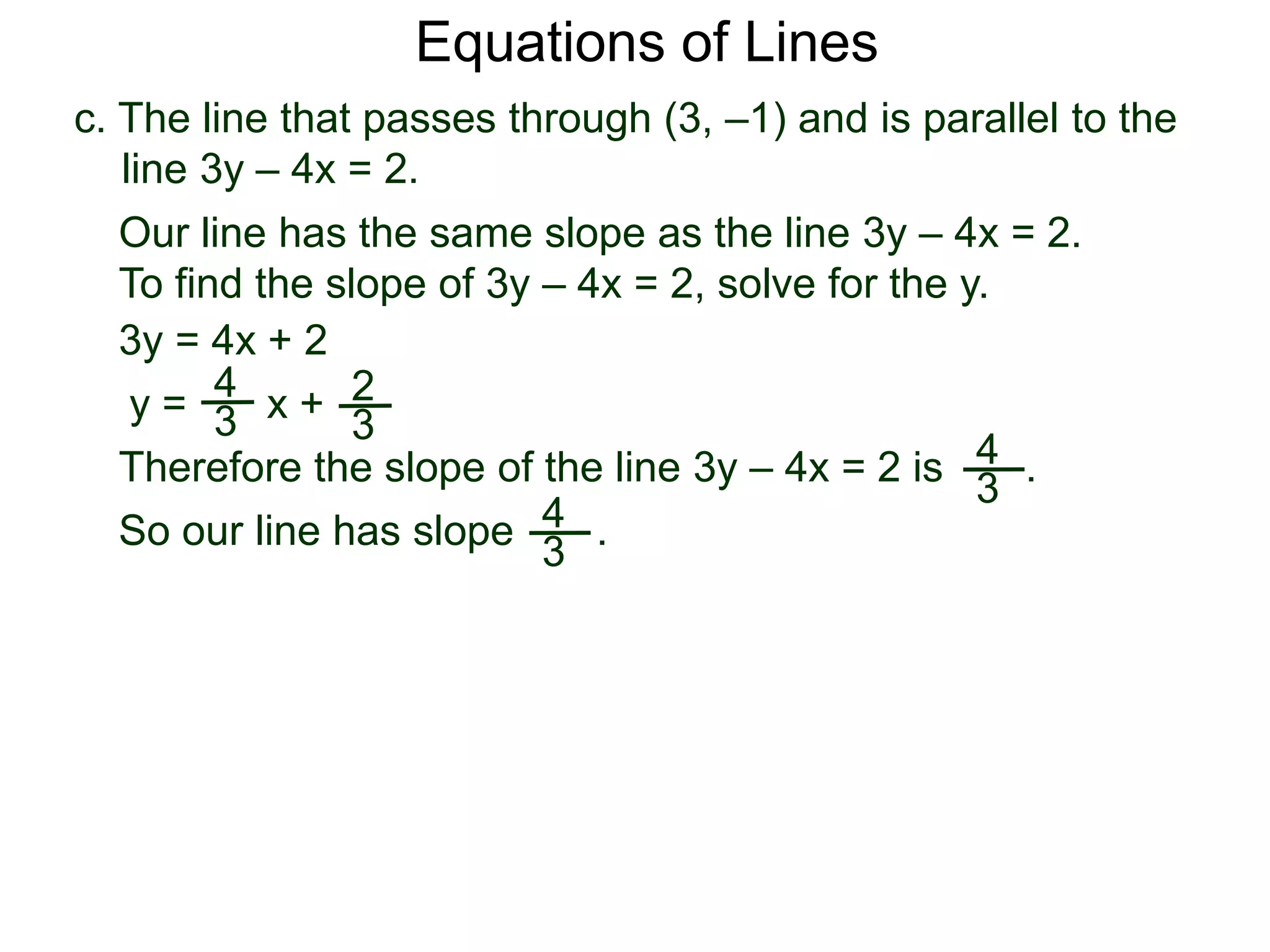
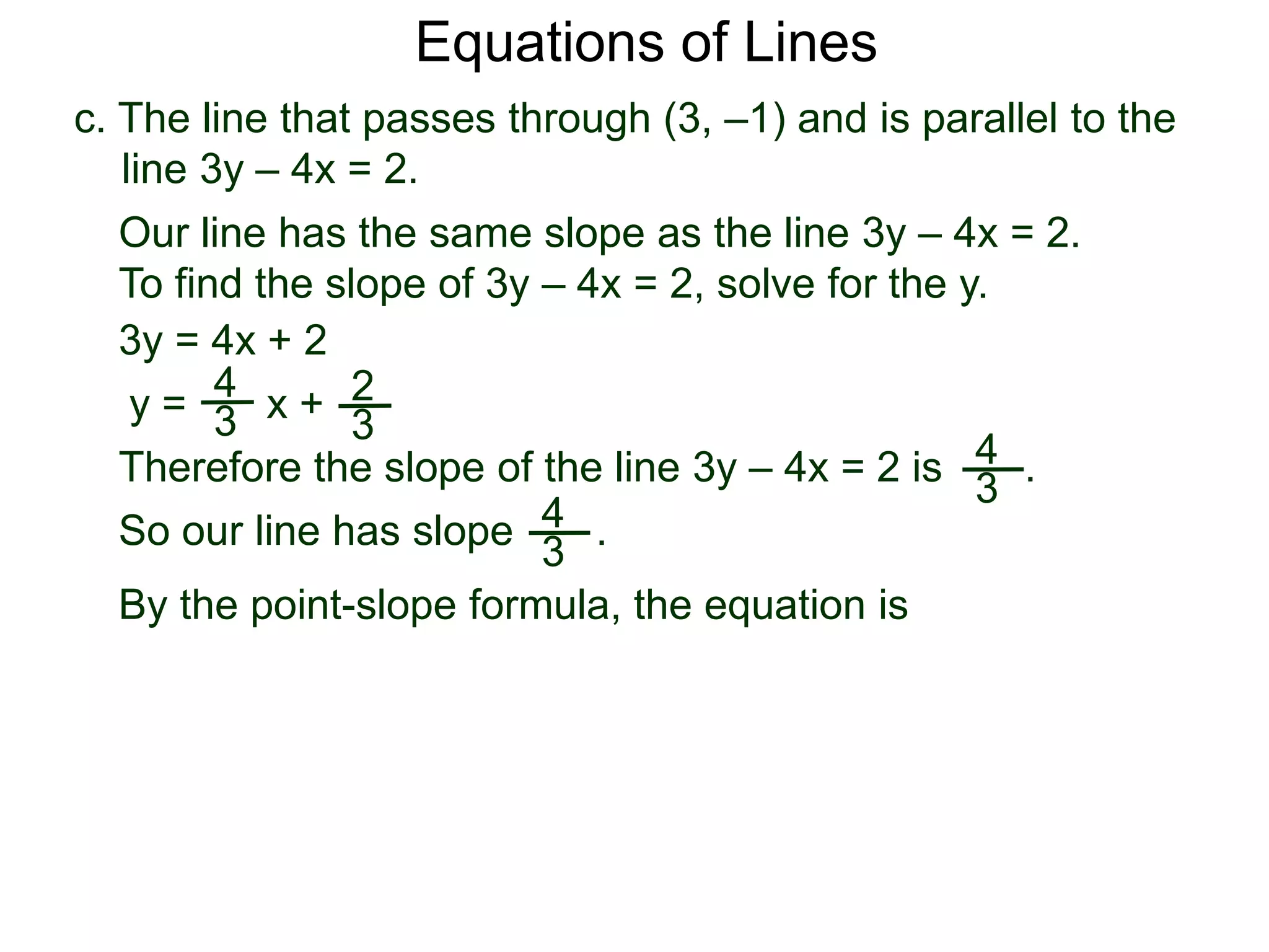
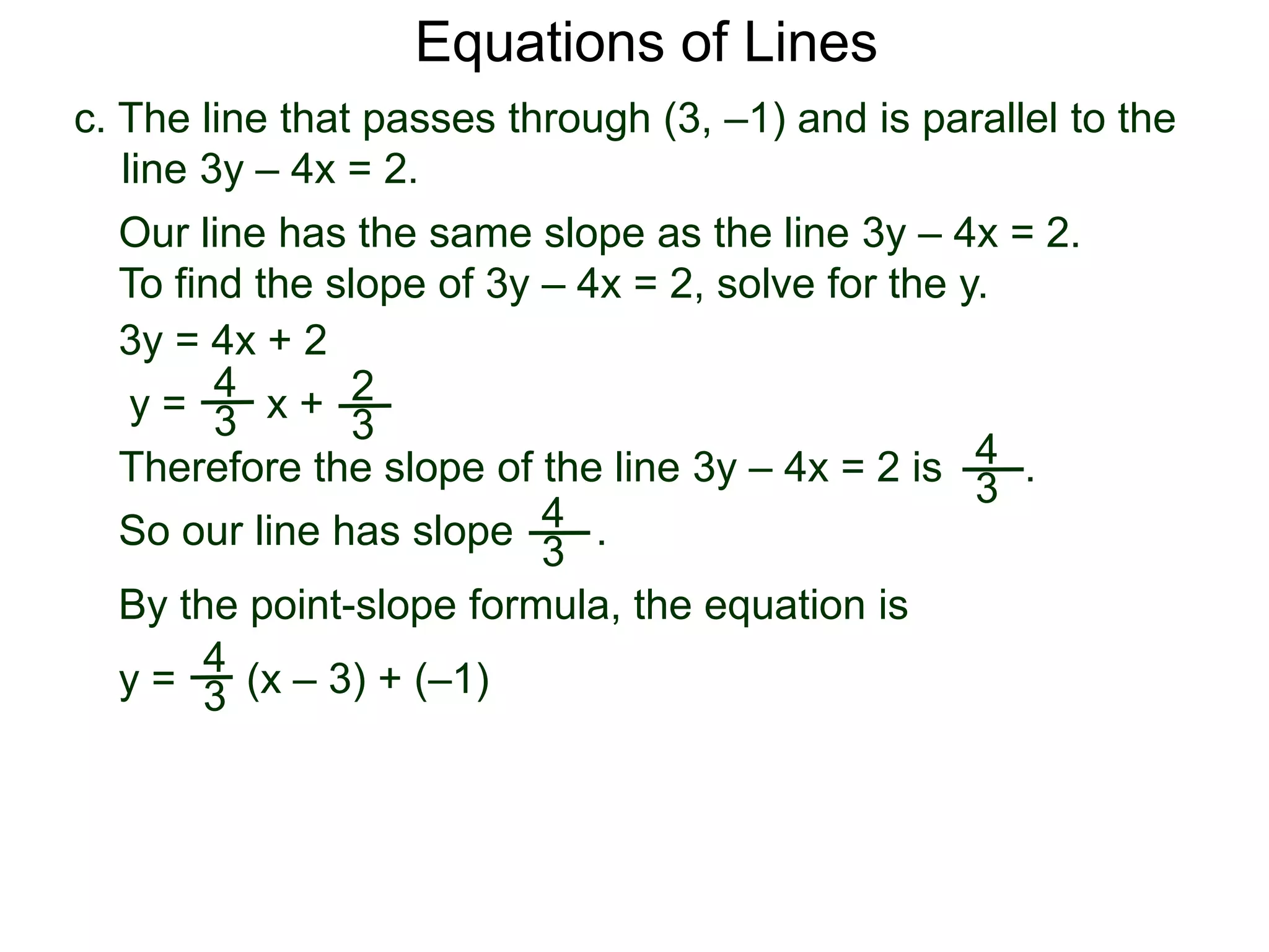
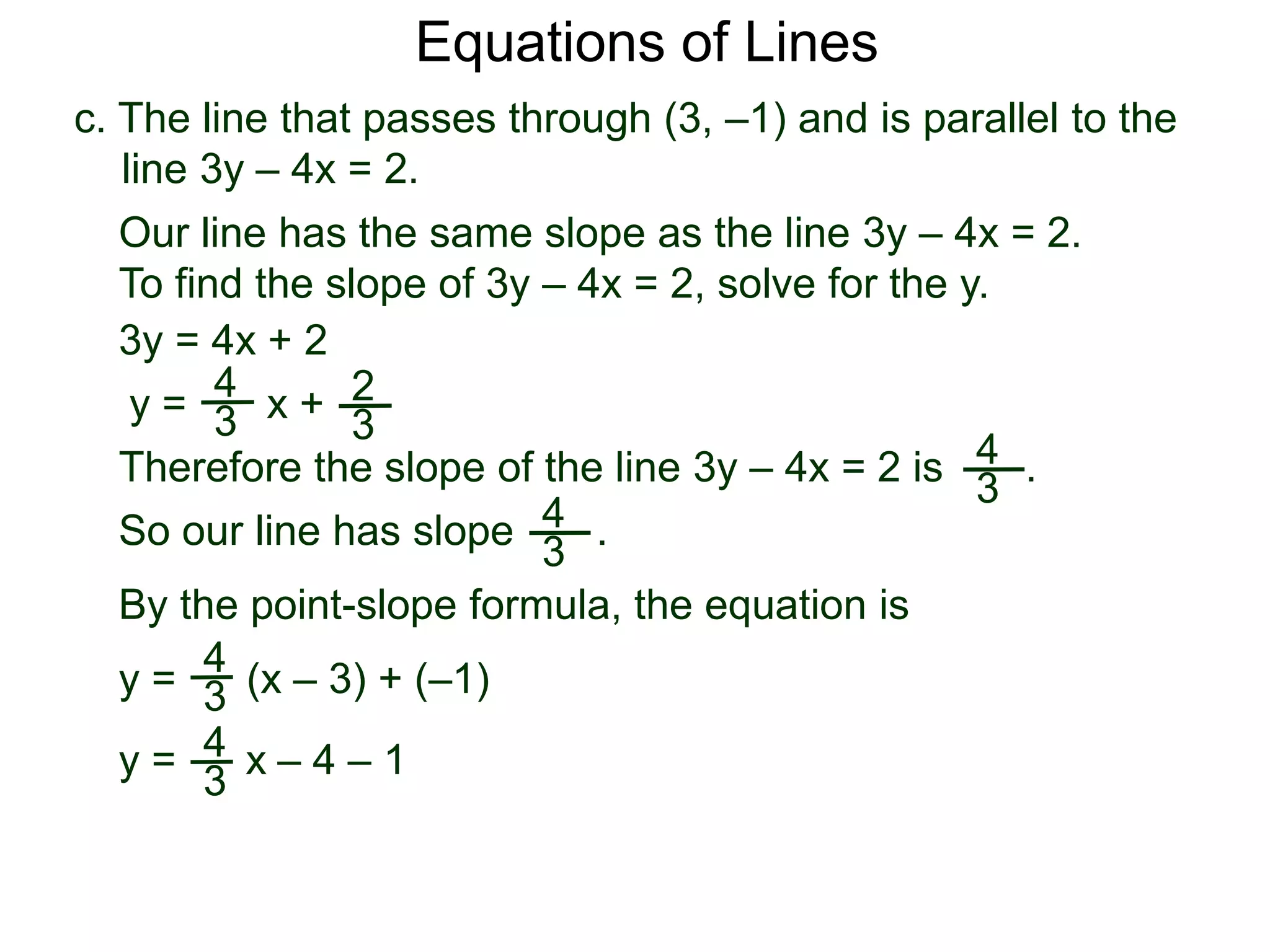
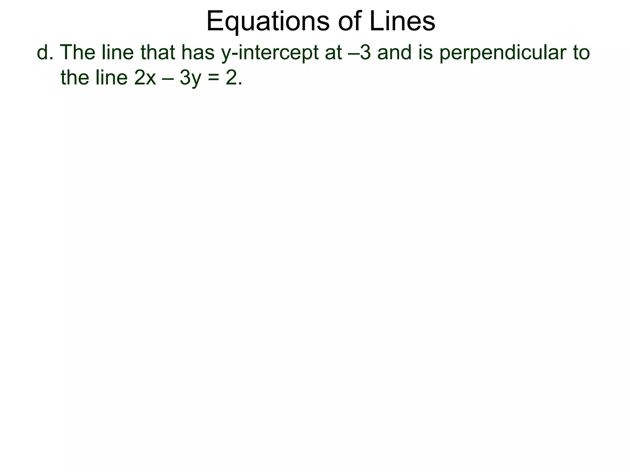
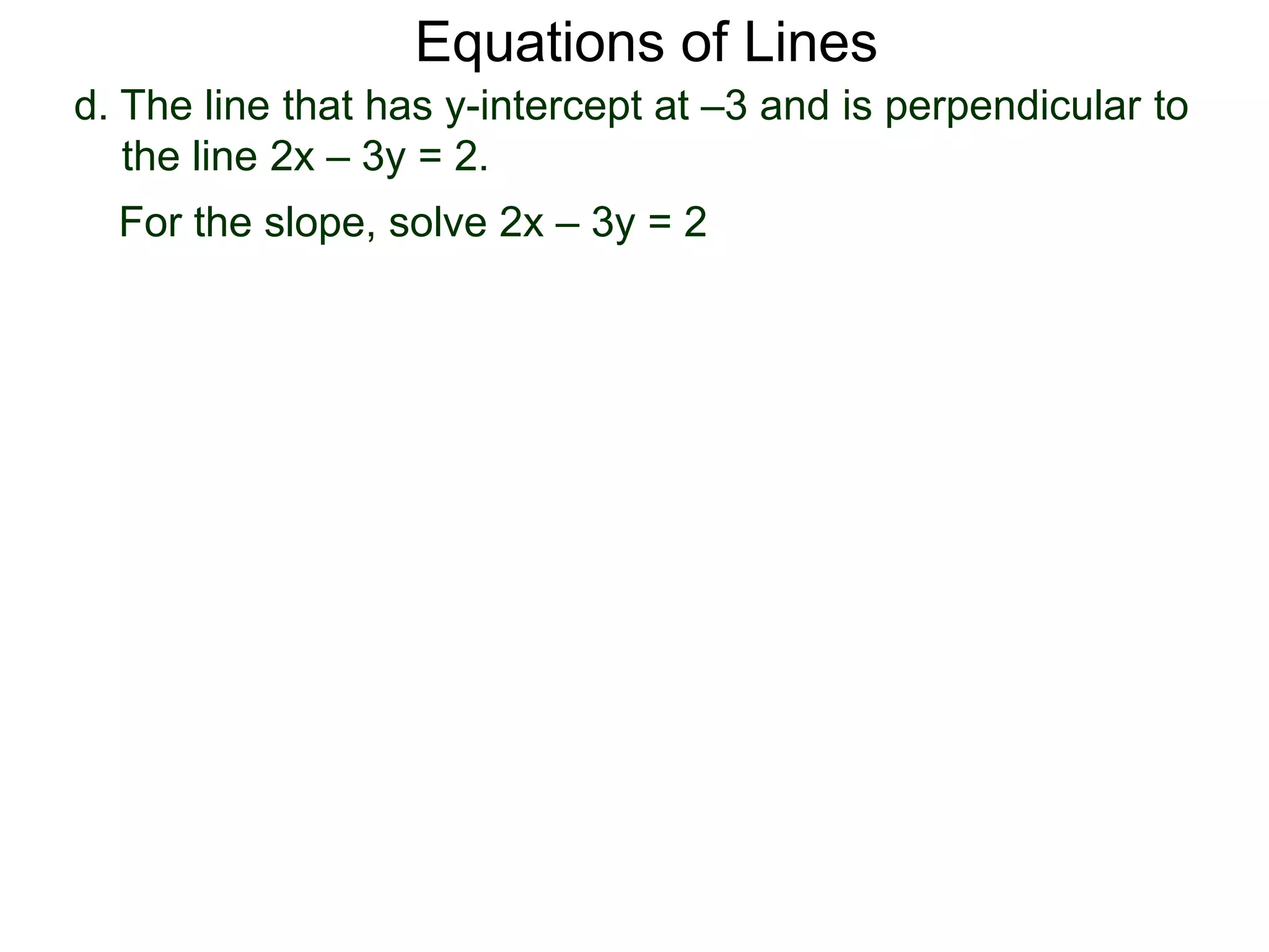
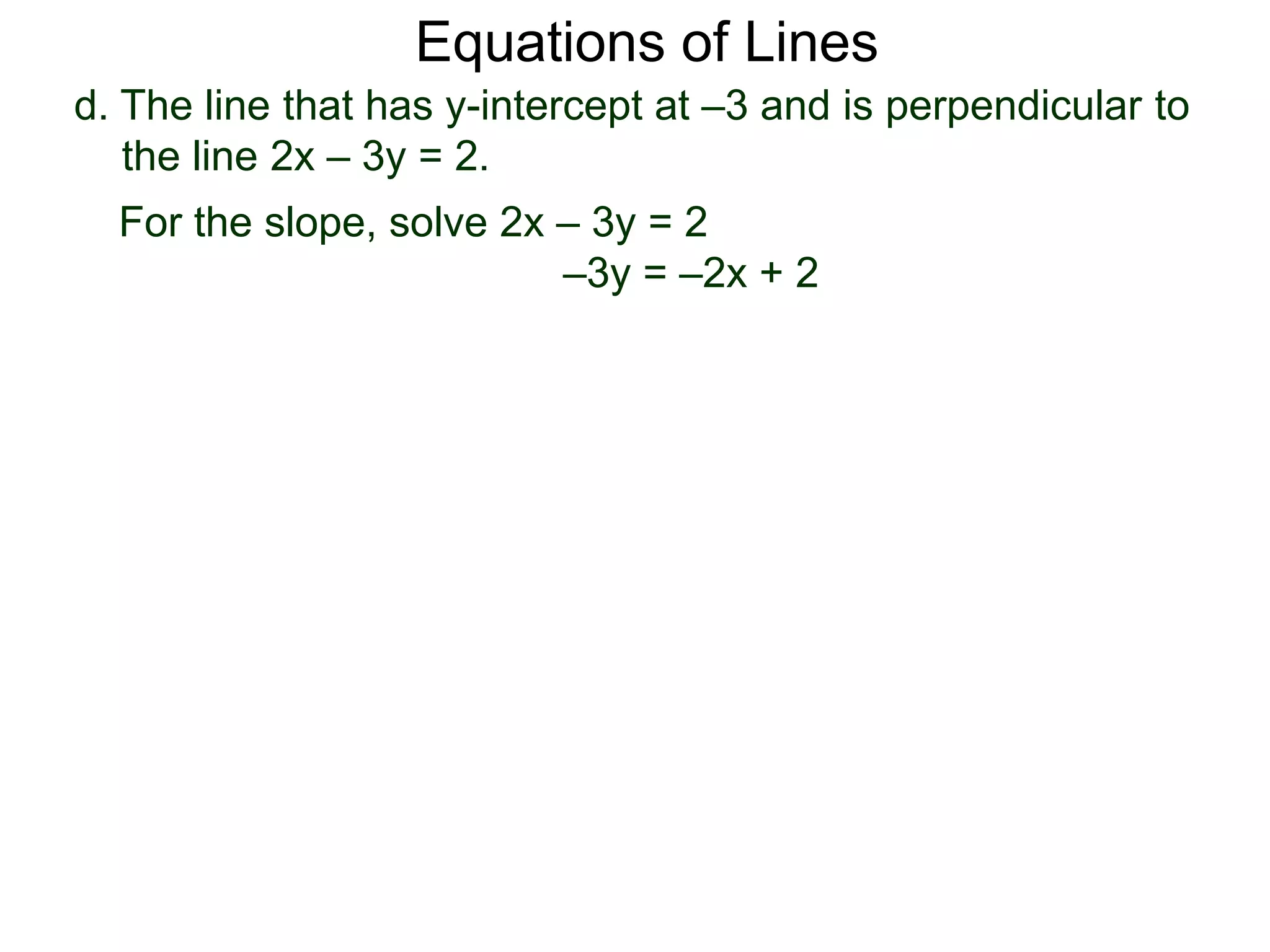
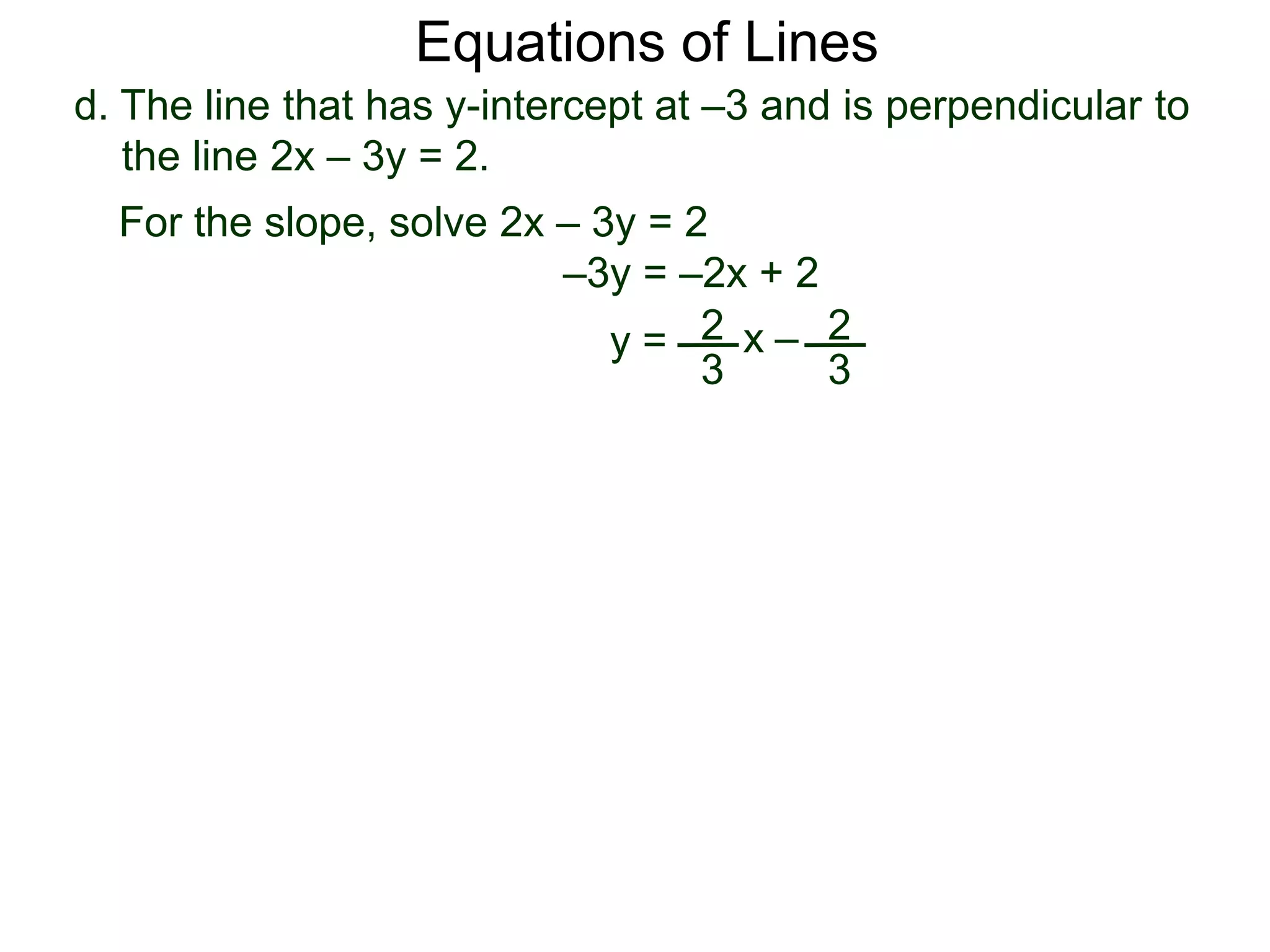
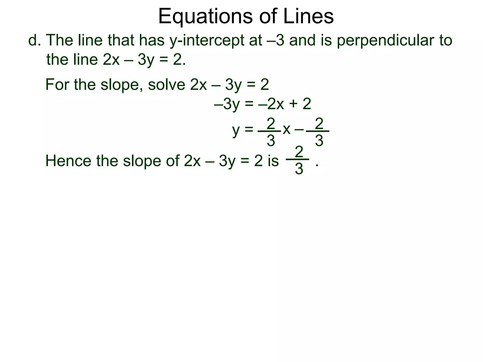
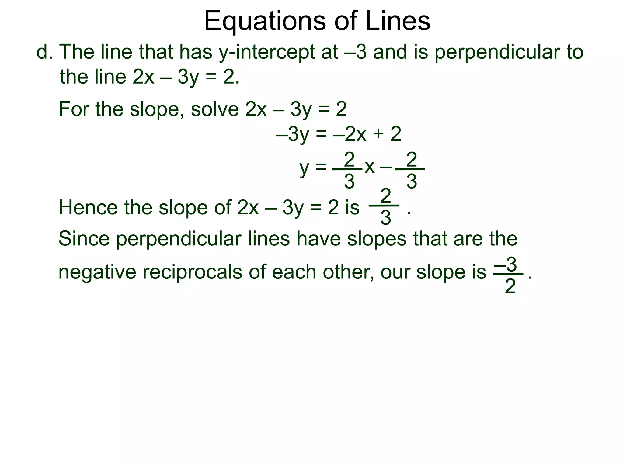
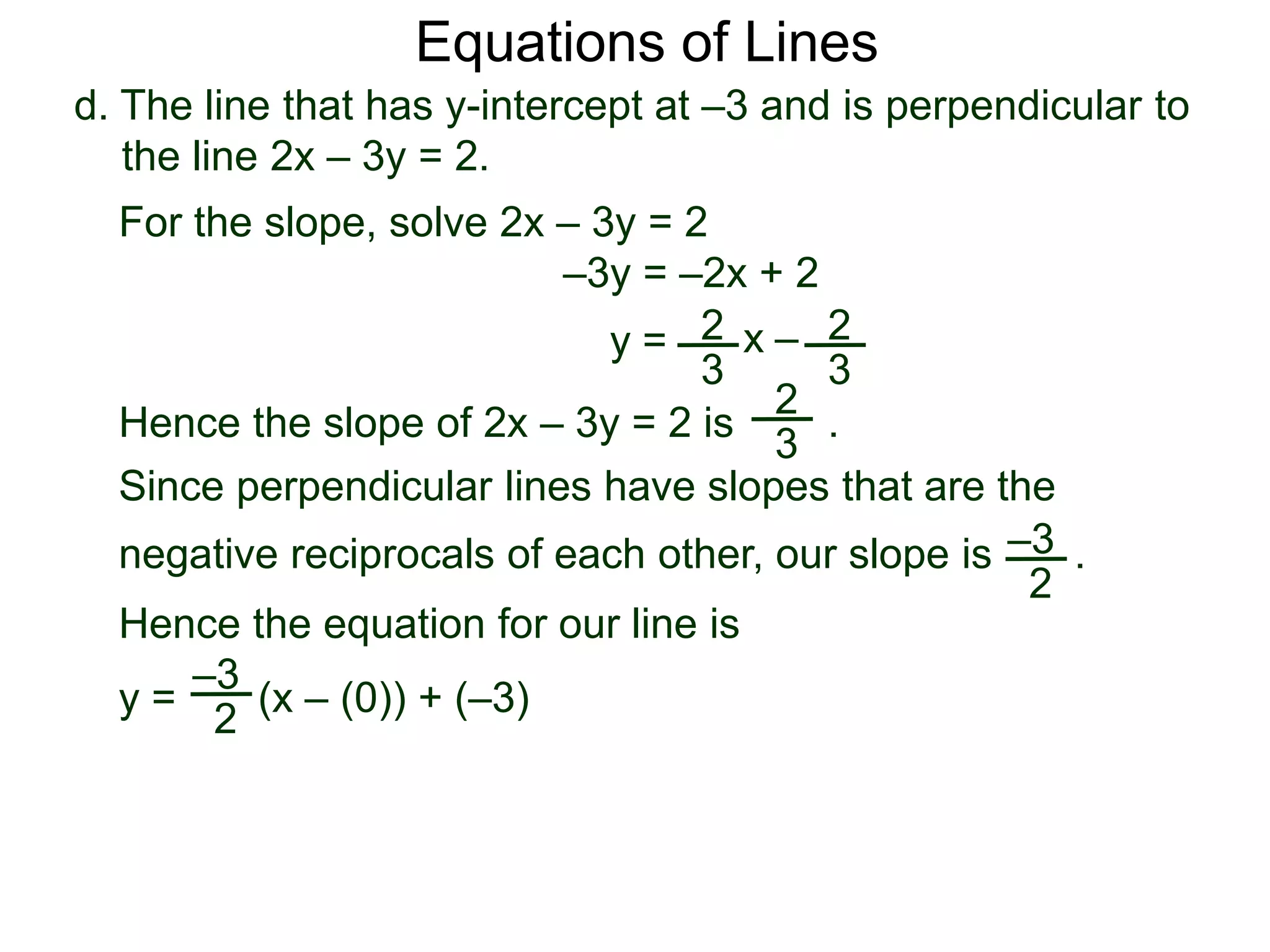
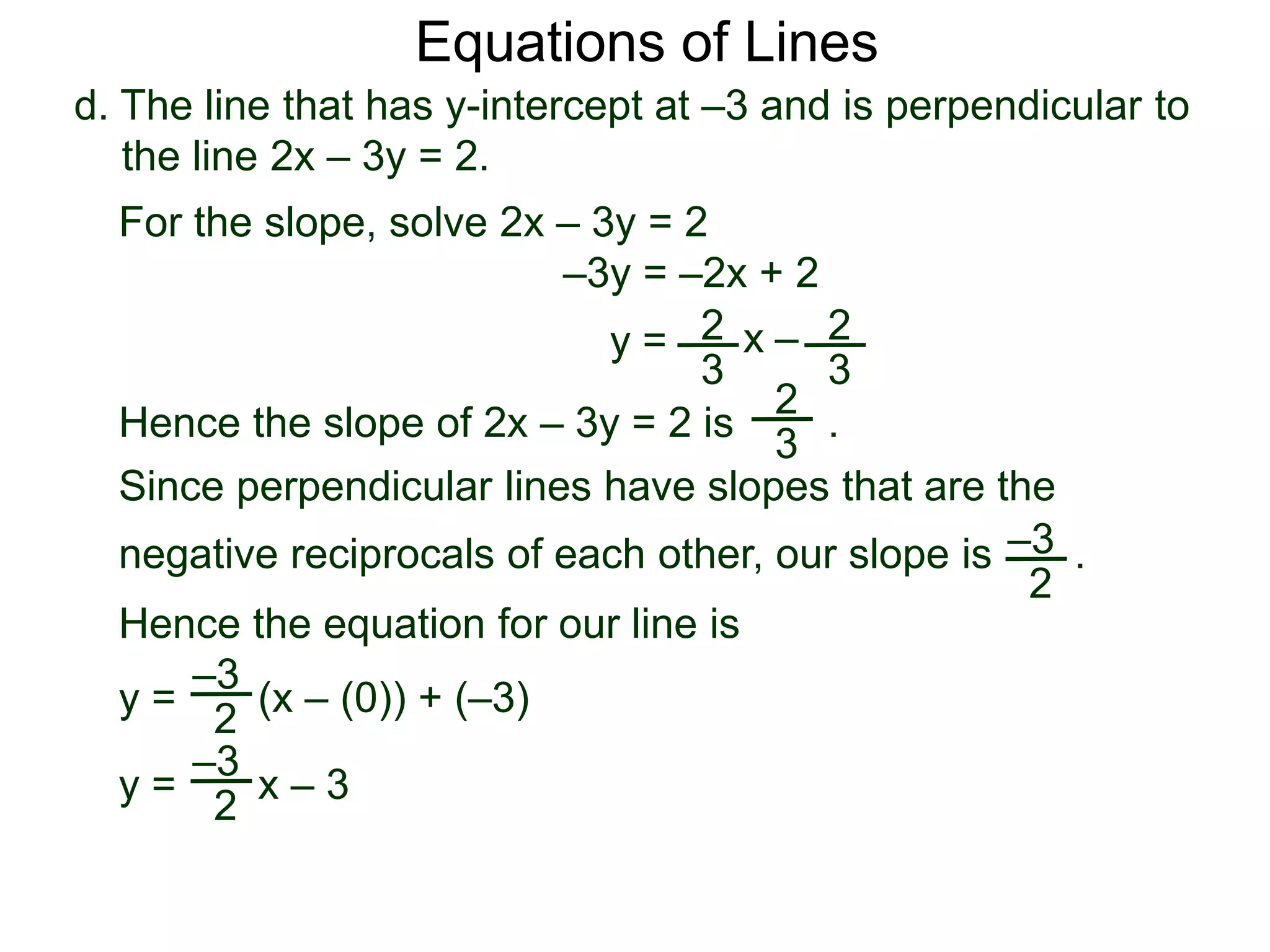
SlideShare a Scribd company logo
1 of 101
Given enough information about a line, we can reconstruct an
equation of the line.
Equations of Lines
Given enough information about a line, we can reconstruct an
equation of the line. We separate them into two cases.
Equations of Lines
Given enough information about a line, we can reconstruct an
equation of the line. We separate them into two cases.
Case I. Horizontal and Vertical Lines (The Special Case)
Equations of Lines
Given enough information about a line, we can reconstruct an
equation of the line. We separate them into two cases.
The slope of horizontal
lines is 0.
Case I. Horizontal and Vertical Lines (The Special Case)
Equations of Lines
Given enough information about a line, we can reconstruct an
equation of the line. We separate them into two cases.
The slope of horizontal
lines is 0. Hence the
equations of
horizontal lines are y = c.
Case I. Horizontal and Vertical Lines (The Special Case)
Equations of Lines
Given enough information about a line, we can reconstruct an
equation of the line. We separate them into two cases.
The slope of horizontal
lines is 0. Hence the
equations of
horizontal lines are y = c.
Case I. Horizontal and Vertical Lines (The Special Case)
y= 3
Equations of Lines
Horizontal lines have slope 0.
Given enough information about a line, we can reconstruct an
equation of the line. We separate them into two cases.
The slope of horizontal
lines is 0. Hence the
equations of
horizontal lines are y = c.
Case I. Horizontal and Vertical Lines (The Special Case)
y= 3
y=1½
Equations of Lines
Horizontal lines have slope 0.
Given enough information about a line, we can reconstruct an
equation of the line. We separate them into two cases.
The slope of horizontal
lines is 0. Hence the
equations of
horizontal lines are y = c.
Case I. Horizontal and Vertical Lines (The Special Case)
y= –3
y= 3
y=1½
Equations of Lines
Horizontal lines have slope 0.
The slope of vertical lines is
undefined, i.e. there is no “y” in
the equation.
Given enough information about a line, we can reconstruct an
equation of the line. We separate them into two cases.
The slope of horizontal
lines is 0. Hence the
equations of
horizontal lines are y = c.
Case I. Horizontal and Vertical Lines (The Special Case)
y= –3
y= 3
y=1½
Equations of Lines
Horizontal lines have slope 0.
The slope of vertical lines is
undefined, i.e. there is no “y” in
the equation. So the equations
of vertical lines are x = c.
Slope of vertical line is undefined.
x= 5
Given enough information about a line, we can reconstruct an
equation of the line. We separate them into two cases.
The slope of horizontal
lines is 0. Hence the
equations of
horizontal lines are y = c.
Case I. Horizontal and Vertical Lines (The Special Case)
y= –3
y= 3
y=1½
Equations of Lines
Horizontal lines have slope 0.
The slope of vertical lines is
undefined, i.e. there is no “y” in
the equation. So the equations
of vertical lines are x = c.
Slope of vertical line is undefined.
x= 2 x= 5
Given enough information about a line, we can reconstruct an
equation of the line. We separate them into two cases.
The slope of horizontal
lines is 0. Hence the
equations of
horizontal lines are y = c.
Case I. Horizontal and Vertical Lines (The Special Case)
y= –3
y= 3
y=1½
Equations of Lines
Horizontal lines have slope 0.
The slope of vertical lines is
undefined, i.e. there is no “y” in
the equation. So the equations
of vertical lines are x = c.
Slope of vertical line is undefined.
x= –4 x= 2 x= 5
Equations of Lines
Example A.
a. A line passes through (3, –1 ),
(3, –3). Draw. Find its equation.
Equations of Lines
Example A.
a. A line passes through (3, –1 ),
(3, –3). Draw. Find its equation.
Equations of Lines
Example A.
a. A line passes through (3, –1 ),
(3, –3). Draw. Find its equation.
Equations of Lines
Example A.
a. A line passes through (3, –1 ),
(3, –3). Draw. Find its equation.
Equations of Lines
Example A.
a. A line passes through (3, –1 ),
(3, –3). Draw. Find its equation.
It’s a vertical line.
Equations of Lines
Example A.
a. A line passes through (3, –1 ),
(3, –3). Draw. Find its equation.
It’s a vertical line. So the
equation is x = c for some c.
Equations of Lines
Example A.
a. A line passes through (3, –1 ),
(3, –3). Draw. Find its equation.
It’s a vertical line. So the
equation is x = c for some c.
Since (3, –1) is on the line so
the equation must be x = 3.
Equations of Lines
Example A.
a. A line passes through (3, –1 ),
(3, –3). Draw. Find its equation.
It’s a vertical line. So the
equation is x = c for some c.
Since (3, –1) is on the line so
the equation must be x = 3.
b. A line passes through (3, –1 )
and it’s parallel to the x-axis.
Draw. Find its equation.
Because it’s parallel to the x-
axis, it must be a horizontal
line.
Equations of Lines
Example A.
a. A line passes through (3, –1 ),
(3, –3). Draw. Find its equation.
It’s a vertical line. So the
equation is x = c for some c.
Since (3, –1) is on the line so
the equation must be x = 3.
b. A line passes through (3, –1 )
and it’s parallel to the x-axis.
Draw. Find its equation.
Because it’s parallel to the x-
axis, it must be a horizontal
line. So the equation is y = c
for some c.
Equations of Lines
Example A.
a. A line passes through (3, –1 ),
(3, –3). Draw. Find its equation.
It’s a vertical line. So the
equation is x = c for some c.
Since (3, –1) is on the line so
the equation must be x = 3.
b. A line passes through (3, –1 )
and it’s parallel to the x-axis.
Draw. Find its equation.
Because it’s parallel to the x-
axis, it must be a horizontal
line. So the equation is y = c
for some c. Since (3, –1) is on
the line so the equation must
be y = –1.
Equations of Lines
Case II. Tilted Lines (The General Case)
Equations of Lines
Case II. Tilted Lines (The General Case)
To find the equations of tilted lines, use the formula below.
Equations of Lines
Case II. Tilted Lines (The General Case)
To find the equations of tilted lines, use the formula below.
It gives the slope-intercept equations directly.
Equations of Lines
Case II. Tilted Lines (The General Case)
To find the equations of tilted lines, use the formula below.
It gives the slope-intercept equations directly. We need the
slope and a point on the line to use this formula.
Equations of Lines
Case II. Tilted Lines (The General Case)
To find the equations of tilted lines, use the formula below.
It gives the slope-intercept equations directly. We need the
slope and a point on the line to use this formula.
The Point Slope Formula (for composing the equations)
Equations of Lines
Case II. Tilted Lines (The General Case)
To find the equations of tilted lines, use the formula below.
It gives the slope-intercept equations directly. We need the
slope and a point on the line to use this formula.
Given the slope m, and a point (x1, y1) on the line,
The Point Slope Formula (for composing the equations)
Equations of Lines
Case II. Tilted Lines (The General Case)
To find the equations of tilted lines, use the formula below.
It gives the slope-intercept equations directly. We need the
slope and a point on the line to use this formula.
Given the slope m, and a point (x1, y1) on the line, then
The Point Slope Formula (for composing the equations)
y = m(x – x1) + y1
is the equation of the line.
Example B. Find the equations of the following lines.
a. The line with slope -2 and y-intercept at -7.
Equations of Lines
Case II. Tilted Lines (The General Case)
To find the equations of tilted lines, use the formula below.
It gives the slope-intercept equations directly. We need the
slope and a point on the line to use this formula.
Given the slope m, and a point (x1, y1) on the line, then
The Point Slope Formula (for composing the equations)
y = m(x – x1) + y1
is the equation of the line.
The slope is –2, the point is (0, –7).
Example B. Find the equations of the following lines.
a. The line with slope -2 and y-intercept at -7.
Equations of Lines
Case II. Tilted Lines (The General Case)
To find the equations of tilted lines, use the formula below.
It gives the slope-intercept equations directly. We need the
slope and a point on the line to use this formula.
Given the slope m, and a point (x1, y1) on the line, then
The Point Slope Formula (for composing the equations)
y = m(x – x1) + y1
is the equation of the line.
The slope is –2, the point is (0, –7). Hence,
y = –2(x
Example B. Find the equations of the following lines.
a. The line with slope -2 and y-intercept at -7.
Equations of Lines
Case II. Tilted Lines (The General Case)
To find the equations of tilted lines, use the formula below.
It gives the slope-intercept equations directly. We need the
slope and a point on the line to use this formula.
Given the slope m, and a point (x1, y1) on the line, then
The Point Slope Formula (for composing the equations)
y = m(x – x1) + y1
is the equation of the line.
The slope is –2, the point is (0, –7). Hence,
y = –2(x – 0)
Example B. Find the equations of the following lines.
a. The line with slope -2 and y-intercept at -7.
Equations of Lines
Case II. Tilted Lines (The General Case)
To find the equations of tilted lines, use the formula below.
It gives the slope-intercept equations directly. We need the
slope and a point on the line to use this formula.
Given the slope m, and a point (x1, y1) on the line, then
The Point Slope Formula (for composing the equations)
y = m(x – x1) + y1
is the equation of the line.
The slope is –2, the point is (0, –7). Hence,
y = –2(x – 0) + (–7)
or y = –2x – 7
Example B. Find the equations of the following lines.
a. The line with slope -2 and y-intercept at -7.
b. The line that contains (1, –2) with the x-intercept at –4.
Equations of Lines
b. The line that contains (1, –2) with the x-intercept at –4.
We have two points on the line (1, –2), (–4, 0) and we
need the slope.
Equations of Lines
b. The line that contains (1, –2) with the x-intercept at –4.
Δy
Δx
We have two points on the line (1, –2), (–4, 0) and we
need the slope. Use the slope formula,
m =
Equations of Lines
b. The line that contains (1, –2) with the x-intercept at –4.
Δy
Δx
0 – (–2 )
–4 – (1)
=
We have two points on the line (1, –2), (–4, 0) and we
need the slope. Use the slope formula,
m =
Equations of Lines
b. The line that contains (1, –2) with the x-intercept at –4.
Δy
Δx
0 – (–2 )
–4 – (1)
2
–5
=
We have two points on the line (1, –2), (–4, 0) and we
need the slope. Use the slope formula,
=m =
Equations of Lines
b. The line that contains (1, –2) with the x-intercept at –4.
Δy
Δx
0 – (–2 )
–4 – (1)
2
–5
=
We have two points on the line (1, –2), (–4, 0) and we
need the slope. Use the slope formula,
=
using the point (–4, 0), plug in the Point Slope Formula
m =
Equations of Lines
y = m(x – x1) + y1
b. The line that contains (1, –2) with the x-intercept at –4.
Δy
Δx
0 – (–2 )
–4 – (1)
2
–5
=
We have two points on the line (1, –2), (–4, 0) and we
need the slope. Use the slope formula,
=
using the point (–4, 0), plug in the Point Slope Formula
m =
Equations of Lines
y = m(x – x1) + y1
b. The line that contains (1, –2) with the x-intercept at –4.
Δy
Δx
0 – (–2 )
–4 – (1)
2
–5
=
y =
We have two points on the line (1, –2), (–4, 0) and we
need the slope. Use the slope formula,
=
using the point (–4, 0), plug in the Point Slope Formula
5
–2
(x – (–4)) + 0
m =
Equations of Lines
b. The line that contains (1, –2) with the x-intercept at –4.
Δy
Δx
0 – (–2 )
–4 – (1)
2
–5
=
y =
We have two points on the line (1, –2), (–4, 0) and we
need the slope. Use the slope formula,
=
using the point (–4, 0), plug in the Point Slope Formula
5
–2
(x – (–4)) + 0
m =
y = (x + 4)
5
–2
y = x –
5
–2 8
5
Equations of Lines
(or 5y = –2x – 8)
b. The line that contains (1, –2) with the x-intercept at –4.
Δy
Δx
0 – (–2 )
–4 – (1)
2
–5
=
y =
We have two points on the line (1, –2), (–4, 0) and we
need the slope. Use the slope formula,
=
using the point (–4, 0), plug in the Point Slope Formula
5
–2
(x – (–4)) + 0
m =
y = (x + 4)
5
–2
y = x –
5
–2 8
5
Equations of Lines
Recall that parallel lines have the same slope and
perpendicular lines have slopes that are the negative
reciprocals of each other.
(or 5y = –2x – 8)
c. The line that passes through (3, –1) and is parallel to the
line 3y – 4x = 2.
Equations of Lines
c. The line that passes through (3, –1) and is parallel to the
line 3y – 4x = 2.
Equations of Lines
Our line has the same slope as the line 3y – 4x = 2.
c. The line that passes through (3, –1) and is parallel to the
line 3y – 4x = 2.
Equations of Lines
Our line has the same slope as the line 3y – 4x = 2.
To find the slope of 3y – 4x = 2, solve for the y.
c. The line that passes through (3, –1) and is parallel to the
line 3y – 4x = 2.
Equations of Lines
Our line has the same slope as the line 3y – 4x = 2.
To find the slope of 3y – 4x = 2, solve for the y.
3y = 4x + 2
c. The line that passes through (3, –1) and is parallel to the
line 3y – 4x = 2.
Equations of Lines
Our line has the same slope as the line 3y – 4x = 2.
To find the slope of 3y – 4x = 2, solve for the y.
3y = 4x + 2
y =
4
3 x + 2
3
c. The line that passes through (3, –1) and is parallel to the
line 3y – 4x = 2.
4
3
Equations of Lines
Our line has the same slope as the line 3y – 4x = 2.
To find the slope of 3y – 4x = 2, solve for the y.
Therefore the slope of the line 3y – 4x = 2 is .
3y = 4x + 2
y =
4
3 x + 2
3
c. The line that passes through (3, –1) and is parallel to the
line 3y – 4x = 2.
4
3
Equations of Lines
Our line has the same slope as the line 3y – 4x = 2.
To find the slope of 3y – 4x = 2, solve for the y.
Therefore the slope of the line 3y – 4x = 2 is .
3y = 4x + 2
y =
4
3 x + 2
3
So our line has slope .4
3
c. The line that passes through (3, –1) and is parallel to the
line 3y – 4x = 2.
4
3
Equations of Lines
Our line has the same slope as the line 3y – 4x = 2.
To find the slope of 3y – 4x = 2, solve for the y.
Therefore the slope of the line 3y – 4x = 2 is .
3y = 4x + 2
y =
4
3 x + 2
3
By the point-slope formula, the equation is
So our line has slope .4
3
c. The line that passes through (3, –1) and is parallel to the
line 3y – 4x = 2.
4
3
Equations of Lines
Our line has the same slope as the line 3y – 4x = 2.
To find the slope of 3y – 4x = 2, solve for the y.
Therefore the slope of the line 3y – 4x = 2 is .
3y = 4x + 2
y =
4
3 x + 2
3
y = (x – 3) + (–1)
By the point-slope formula, the equation is
So our line has slope .4
3
4
3
y = 4
3
x – 4 – 1
d. The line that has y-intercept at –3 and is perpendicular to
the line 2x – 3y = 2.
Equations of Lines
d. The line that has y-intercept at –3 and is perpendicular to
the line 2x – 3y = 2.
Equations of Lines
For the slope, solve 2x – 3y = 2
d. The line that has y-intercept at –3 and is perpendicular to
the line 2x – 3y = 2.
Equations of Lines
For the slope, solve 2x – 3y = 2
–3y = –2x + 2
d. The line that has y-intercept at –3 and is perpendicular to
the line 2x – 3y = 2.
2
3
Equations of Lines
For the slope, solve 2x – 3y = 2
–3y = –2x + 2
y = 2
3
x –
d. The line that has y-intercept at –3 and is perpendicular to
the line 2x – 3y = 2.
2
3
Equations of Lines
For the slope, solve 2x – 3y = 2
–3y = –2x + 2
y = 2
3
x –
Hence the slope of 2x – 3y = 2 is .
2
3
d. The line that has y-intercept at –3 and is perpendicular to
the line 2x – 3y = 2.
2
3
Equations of Lines
For the slope, solve 2x – 3y = 2
–3y = –2x + 2
y =
Since perpendicular lines have slopes that are the
negative reciprocals of each other, our slope is .
2
3
x –
Hence the slope of 2x – 3y = 2 is .
2
3
–3
2
d. The line that has y-intercept at –3 and is perpendicular to
the line 2x – 3y = 2.
2
3
Equations of Lines
For the slope, solve 2x – 3y = 2
–3y = –2x + 2
y = 2
3
x –
Hence the slope of 2x – 3y = 2 is .
2
3
Hence the equation for our line is
y = (x – (0)) + (–3)
–3
2
Since perpendicular lines have slopes that are the
negative reciprocals of each other, our slope is .–3
2
d. The line that has y-intercept at –3 and is perpendicular to
the line 2x – 3y = 2.
2
3
Equations of Lines
For the slope, solve 2x – 3y = 2
–3y = –2x + 2
y = 2
3
x –
Hence the slope of 2x – 3y = 2 is .
2
3
Hence the equation for our line is
y = (x – (0)) + (–3)
–3
2
y = x – 3
–3
2
Since perpendicular lines have slopes that are the
negative reciprocals of each other, our slope is .–3
2
Linear Equations and Lines
Many real world relations between two quantities are linear.
For example the cost $y is a linear formula of x–the number
of apples bought.
Linear Equations and Lines
Many real world relations between two quantities are linear.
For example the cost $y is a linear formula of x–the number
of apples bought. For those relations that we don’t know
whether they are linear or not, linear formulas give us the
most basic “educated guesses”.
Linear Equations and Lines
Many real world relations between two quantities are linear.
For example the cost $y is a linear formula of x–the number
of apples bought. For those relations that we don’t know
whether they are linear or not, linear formulas give us the
most basic “educated guesses”. The following example
demonstrates that these problems are pondered by people
ancient or present alike.
Linear Equations and Lines
Example C. We live by a river that floods regularly. On a rock
by the river bank there is a mark indicating the highest point
the water level ever reached in the recorded time.
Many real world relations between two quantities are linear.
For example the cost $y is a linear formula of x–the number
of apples bought. For those relations that we don’t know
whether they are linear or not, linear formulas give us the
most basic “educated guesses”. The following example
demonstrates that these problems are pondered by people
ancient or present alike.
Linear Equations and Lines
Example C. We live by a river that floods regularly. On a rock
by the river bank there is a mark indicating the highest point
the water level ever reached in the recorded time. At 12 pm
on July 11, the water level is 28 inches from this mark.
At 8 am on July 12 the water is 18 inches from this mark.
Many real world relations between two quantities are linear.
For example the cost $y is a linear formula of x–the number
of apples bought. For those relations that we don’t know
whether they are linear or not, linear formulas give us the
most basic “educated guesses”. The following example
demonstrates that these problems are pondered by people
ancient or present alike.
Linear Equations and Lines
Example C. We live by a river that floods regularly. On a rock
by the river bank there is a mark indicating the highest point
the water level ever reached in the recorded time. At 12 pm
on July 11, the water level is 28 inches from this mark.
At 8 am on July 12 the water is 18 inches from this mark. Let
x be a measurement for time, and y be the distance from the
water level and the mark.
Many real world relations between two quantities are linear.
For example the cost $y is a linear formula of x–the number
of apples bought. For those relations that we don’t know
whether they are linear or not, linear formulas give us the
most basic “educated guesses”. The following example
demonstrates that these problems are pondered by people
ancient or present alike.
Linear Equations and Lines
Example C. We live by a river that floods regularly. On a rock
by the river bank there is a mark indicating the highest point
the water level ever reached in the recorded time. At 12 pm
on July 11, the water level is 28 inches from this mark.
At 8 am on July 12 the water is 18 inches from this mark. Let
x be a measurement for time, and y be the distance from the
water level and the mark. Find the linear equation between x
and y.
Many real world relations between two quantities are linear.
For example the cost $y is a linear formula of x–the number
of apples bought. For those relations that we don’t know
whether they are linear or not, linear formulas give us the
most basic “educated guesses”. The following example
demonstrates that these problems are pondered by people
ancient or present alike.
Linear Equations and Lines
Example C. We live by a river that floods regularly. On a rock
by the river bank there is a mark indicating the highest point
the water level ever reached in the recorded time. At 12 pm
on July 11, the water level is 28 inches from this mark.
At 8 am on July 12 the water is 18 inches from this mark. Let
x be a measurement for time, and y be the distance from the
water level and the mark. Find the linear equation between x
and y. At 4 pm July 12, the water level is 12 inches from the
mark, is the flood easing or intensifying?
Many real world relations between two quantities are linear.
For example the cost $y is a linear formula of x–the number
of apples bought. For those relations that we don’t know
whether they are linear or not, linear formulas give us the
most basic “educated guesses”. The following example
demonstrates that these problems are pondered by people
ancient or present alike.
Equations of Lines
The easiest way to set the time measurement x is to set
x = 0 (hr) to the time of the first observation.
Equations of Lines
The easiest way to set the time measurement x is to set
x = 0 (hr) to the time of the first observation. Hence set x = 0
at 12 pm July 11.
Equations of Lines
The easiest way to set the time measurement x is to set
x = 0 (hr) to the time of the first observation. Hence set x = 0
at 12 pm July 11. Therefore at 8 am of July 12, x = 20.
Equations of Lines
The easiest way to set the time measurement x is to set
x = 0 (hr) to the time of the first observation. Hence set x = 0
at 12 pm July 11. Therefore at 8 am of July 12, x = 20.
In particular, we are given that at x = 0, y = 28, and at
x = 20, y = 18.
Equations of Lines
The easiest way to set the time measurement x is to set
x = 0 (hr) to the time of the first observation. Hence set x = 0
at 12 pm July 11. Therefore at 8 am of July 12, x = 20.
In particular, we are given that at x = 0, y = 28, and at
x = 20, y = 18. We want the equation y = m(x – x1) + y1
of the line that contains the points (0, 28) and (20, 18).
The slope m = = = –1/2
Δy
Δx
28 – 18
0 – 20
Equations of Lines
The easiest way to set the time measurement x is to set
x = 0 (hr) to the time of the first observation. Hence set x = 0
at 12 pm July 11. Therefore at 8 am of July 12, x = 20.
In particular, we are given that at x = 0, y = 28, and at
x = 20, y = 18. We want the equation y = m(x – x1) + y1
of the line that contains the points (0, 28) and (20, 18).
The slope m = = = –1/2
Hence the linear equation is y = –1/2(x – 0) + 28 or that
y = – + 28
Δy
Δx
28 – 18
0 – 20
2
Equations of Lines
The easiest way to set the time measurement x is to set
x = 0 (hr) to the time of the first observation. Hence set x = 0
at 12 pm July 11. Therefore at 8 am of July 12, x = 20.
In particular, we are given that at x = 0, y = 28, and at
x = 20, y = 18. We want the equation y = m(x – x1) + y1
of the line that contains the points (0, 28) and (20, 18).
x
At 4 pm July 12, x = 28.
The slope m = = = –1/2
Hence the linear equation is y = –1/2(x – 0) + 28 or that
y = – + 28
Δy
Δx
28 – 18
0 – 20
2
Equations of Lines
The easiest way to set the time measurement x is to set
x = 0 (hr) to the time of the first observation. Hence set x = 0
at 12 pm July 11. Therefore at 8 am of July 12, x = 20.
In particular, we are given that at x = 0, y = 28, and at
x = 20, y = 18. We want the equation y = m(x – x1) + y1
of the line that contains the points (0, 28) and (20, 18).
x
At 4 pm July 12, x = 28. According to the formula
y = – 28/2 + 28 = –14 + 28 = 14.
The slope m = = = –1/2
Hence the linear equation is y = –1/2(x – 0) + 28 or that
y = – + 28
Δy
Δx
28 – 18
0 – 20
2
Equations of Lines
The easiest way to set the time measurement x is to set
x = 0 (hr) to the time of the first observation. Hence set x = 0
at 12 pm July 11. Therefore at 8 am of July 12, x = 20.
In particular, we are given that at x = 0, y = 28, and at
x = 20, y = 18. We want the equation y = m(x – x1) + y1
of the line that contains the points (0, 28) and (20, 18).
x
At 4 pm July 12, x = 28. According to the formula
y = – 28/2 + 28 = –14 + 28 = 14. But our actual observation,
the water level is only 12 inches from the mark.
Hence the flood is intensifying.
The slope m = = = –1/2
Hence the linear equation is y = –1/2(x – 0) + 28 or that
y = – + 28
Δy
Δx
28 – 18
0 – 20
2
Equations of Lines
The easiest way to set the time measurement x is to set
x = 0 (hr) to the time of the first observation. Hence set x = 0
at 12 pm July 11. Therefore at 8 am of July 12, x = 20.
In particular, we are given that at x = 0, y = 28, and at
x = 20, y = 18. We want the equation y = m(x – x1) + y1
of the line that contains the points (0, 28) and (20, 18).
x
At 4 pm July 12, x = 28. According to the formula
y = – 28/2 + 28 = –14 + 28 = 14. But our actual observation,
the water level is only 12 inches from the mark.
Hence the flood is intensifying. The linear equation that we
found is also called a trend line and it is shown below.
Linear Equations and Lines
x = number of hours passed since 12 pm July 11
y = distance from the water level to the high mark
10
20
30
10 20 30
y
40 50
x
(0, 28) y = –x/2 + 28
(20, 18)
Linear Equations and Lines
x = number of hours passed since 12 pm July 11
y = distance from the water level to the high mark
10
20
30
10 20 30
y
40 50
x
(0, 28)
(20, 18)
y = –x/2 + 28
(28, 14)
The projected distance
for 4 pm July 12
Linear Equations and Lines
x = number of hours passed since 12 pm July 11
y = distance from the water level to the high mark
10
20
30
10 20 30
y
40 50
x
(0, 28)
(20, 18)
y = –x/2 + 28
(28, 14)
The projected distance
for 4 pm July 12
(28, 14)
The actual data
taken at 4 pm July 12
Linear Equations and Lines
Exercise A. For problems 1–8 select two points and estimate
the slope, and find an equation of each line.
1. 2. 3. 4.
5. 6. 7. 8.
Linear Equations and Lines
Exercise B. Draw each line that passes through the given two
points. Find the slope and an equation of the line. Identify the
vertical lines and the horizontal lines by inspection first.
9. (0, –1), (–2, 1) 10. (1, –2), (–2, 0) 11. (1, –2), (–2, –1)
12. (3, –1), (3, 1) 13. (1, –2), (–2, 3) 14. (2, –1), (3, –1)
15. (4, –2), (–3, 1) 16. (4, –2), (4, 0) 17. (7, –2), (–2, –6)
18. (3/2, –1), (3/2, 1) 19. (3/2, –1), (1, –3/2)
20. (–5/2, –1/2), (1/2, 1) 21. (3/2, 1/3), (1/3, 1/3)
23. (3/4, –1/3), (1/3, 3/2)
Exercise C. Find the equations of the following lines.
24. The line that passes through (0, 1) and has slope 3.
25. The line that passes through (–2 ,1) and has slope –1/2.
26. The line that passes through (5, 2) and is parallel to y = x.
27. The line that passes through (–3, 2) and is perpendicular
to –x = 2y.
22. (–1/4, –5/6), (2/3, –3/2)
Linear Equations and Lines
Exercise D.
Find the equations of the following lines.
28. The line that passes through (0, 1), (1, –2)
31. It’s perpendicular to 2x – 4y = 1 and passes through (–2, 1)
29. 30.
32. It’s perpendicular to 3y = x with x–intercept at x = –3.
33. It has y–intercept at y = 3 and is parallel to 3y + 4x = 1.
34. It’s perpendicular to the y–axis with y–intercept at 4.
35. It has y–intercept at y = 3 and is parallel to the x axis.
36. It’s perpendicular to the x– axis containing the point (4, –3).
37. It is parallel to the y axis has x–intercept at x = –7.
38. It is parallel to the x axis has y–intercept at y = 7.
Linear Equations and Lines
The cost y of renting a tour boat consists of a base–cost plus
the number of tourists x. With 4 tourists the total cost is $65,
with 11 tourists the total is $86.
39. What is the base cost and what is the charge per tourist?
40. Find the equation of y in terms of x.
41. What is the total cost if there are 28 tourists?
The temperature y of water in a glass is rising slowly.
After 4 min. the temperature is 30 Co, and after 11 min. the
temperature is up to 65 Co. Answer 42–44 assuming the
temperature is rising linearly.
42. What is the temperature at time 0 and what is the rate of
the temperature rise?
43. Find the equation of y in terms of time.
44. How long will it take to bring the water to a boil at 100 Co?
Linear Equations and Lines
The cost of gas y on May 3 is $3.58 and on May 9 is $4.00.
Answer 45–47 assuming the price is rising linearly.
45. Let x be the date in May, what is the rate of increase in
price in terms of x?
46. Find the equation of the price in term of the date x in May.
47. What is the projected price on May 20?
48. In 2005, the most inexpensive tablet cost $900. In the year
2010, it was $500. Find the equation of the price p in terms of
time t. What is the projected price in the year 2014?

More Related Content

What's hot

Pamimili ng iba’t ibang pagkain
Pamimili  ng iba’t ibang pagkainPamimili  ng iba’t ibang pagkain
Pamimili ng iba’t ibang pagkainGracila Dandoy
 
BANGHAY ARALIN SA ARALING PANLIPUNAN V.docx
BANGHAY ARALIN SA ARALING PANLIPUNAN V.docxBANGHAY ARALIN SA ARALING PANLIPUNAN V.docx
BANGHAY ARALIN SA ARALING PANLIPUNAN V.docxJesonAyahayLongno
 
Lesson 51 Identifying and Describing Triangles marvietblanco.pptx
Lesson 51 Identifying and Describing Triangles marvietblanco.pptxLesson 51 Identifying and Describing Triangles marvietblanco.pptx
Lesson 51 Identifying and Describing Triangles marvietblanco.pptxGeraldine Reyes
 
Proportion and how to solve problems in ratio
Proportion and how to solve problems in ratioProportion and how to solve problems in ratio
Proportion and how to solve problems in ratioart bermoy
 
Lecture 2: Biological Aspect of Postharvest Handling of Crops
Lecture 2: Biological Aspect of Postharvest Handling of CropsLecture 2: Biological Aspect of Postharvest Handling of Crops
Lecture 2: Biological Aspect of Postharvest Handling of CropsKarl Obispo
 
Epp 6 industrial arts 3rd quarter- mga gawaing pang-industriya
Epp 6 industrial arts 3rd quarter- mga gawaing pang-industriyaEpp 6 industrial arts 3rd quarter- mga gawaing pang-industriya
Epp 6 industrial arts 3rd quarter- mga gawaing pang-industriyaArnel Bautista
 
EPP 5- AGRI- Week2 Day1-Pagdidilig ng Halaman
EPP 5- AGRI- Week2 Day1-Pagdidilig ng HalamanEPP 5- AGRI- Week2 Day1-Pagdidilig ng Halaman
EPP 5- AGRI- Week2 Day1-Pagdidilig ng HalamanVIRGINITAJOROLAN1
 
Agriculture EPP5
Agriculture EPP5Agriculture EPP5
Agriculture EPP5Arnel Dalit
 
Math iv converting square cm to square m and vice versa
Math iv   converting square cm to square m and vice versaMath iv   converting square cm to square m and vice versa
Math iv converting square cm to square m and vice versaCristy Melloso
 
Kahalagahan ng pagtatanim
Kahalagahan ng pagtatanimKahalagahan ng pagtatanim
Kahalagahan ng pagtatanimElaine Estacio
 
TRIANGLE CONGRUENCE -M8GE-IIId-1.pptx
TRIANGLE CONGRUENCE -M8GE-IIId-1.pptxTRIANGLE CONGRUENCE -M8GE-IIId-1.pptx
TRIANGLE CONGRUENCE -M8GE-IIId-1.pptxNolzkieCaliso
 
Plotting of Points on the Coordinate Plane
Plotting of Points on the Coordinate PlanePlotting of Points on the Coordinate Plane
Plotting of Points on the Coordinate PlaneJoey Valdriz
 

What's hot (20)

PE MELCs Grade 5.pdf
PE MELCs Grade 5.pdfPE MELCs Grade 5.pdf
PE MELCs Grade 5.pdf
 
Pamimili ng iba’t ibang pagkain
Pamimili  ng iba’t ibang pagkainPamimili  ng iba’t ibang pagkain
Pamimili ng iba’t ibang pagkain
 
detailed-lesson-plan-math-9.pdf
detailed-lesson-plan-math-9.pdfdetailed-lesson-plan-math-9.pdf
detailed-lesson-plan-math-9.pdf
 
BANGHAY ARALIN SA ARALING PANLIPUNAN V.docx
BANGHAY ARALIN SA ARALING PANLIPUNAN V.docxBANGHAY ARALIN SA ARALING PANLIPUNAN V.docx
BANGHAY ARALIN SA ARALING PANLIPUNAN V.docx
 
Lesson 51 Identifying and Describing Triangles marvietblanco.pptx
Lesson 51 Identifying and Describing Triangles marvietblanco.pptxLesson 51 Identifying and Describing Triangles marvietblanco.pptx
Lesson 51 Identifying and Describing Triangles marvietblanco.pptx
 
Proportion and how to solve problems in ratio
Proportion and how to solve problems in ratioProportion and how to solve problems in ratio
Proportion and how to solve problems in ratio
 
Lesson plan of similarity
Lesson plan of similarityLesson plan of similarity
Lesson plan of similarity
 
Lecture 2: Biological Aspect of Postharvest Handling of Crops
Lecture 2: Biological Aspect of Postharvest Handling of CropsLecture 2: Biological Aspect of Postharvest Handling of Crops
Lecture 2: Biological Aspect of Postharvest Handling of Crops
 
Epp 6 industrial arts 3rd quarter- mga gawaing pang-industriya
Epp 6 industrial arts 3rd quarter- mga gawaing pang-industriyaEpp 6 industrial arts 3rd quarter- mga gawaing pang-industriya
Epp 6 industrial arts 3rd quarter- mga gawaing pang-industriya
 
EPP 5- AGRI- Week2 Day1-Pagdidilig ng Halaman
EPP 5- AGRI- Week2 Day1-Pagdidilig ng HalamanEPP 5- AGRI- Week2 Day1-Pagdidilig ng Halaman
EPP 5- AGRI- Week2 Day1-Pagdidilig ng Halaman
 
Mathematics 8 Reasoning
Mathematics 8 ReasoningMathematics 8 Reasoning
Mathematics 8 Reasoning
 
Agriculture EPP5
Agriculture EPP5Agriculture EPP5
Agriculture EPP5
 
Measurement
MeasurementMeasurement
Measurement
 
Grafting manual
Grafting manualGrafting manual
Grafting manual
 
Math iv converting square cm to square m and vice versa
Math iv   converting square cm to square m and vice versaMath iv   converting square cm to square m and vice versa
Math iv converting square cm to square m and vice versa
 
Methods of planting
Methods of plantingMethods of planting
Methods of planting
 
Land preparation.pptx
Land preparation.pptxLand preparation.pptx
Land preparation.pptx
 
Kahalagahan ng pagtatanim
Kahalagahan ng pagtatanimKahalagahan ng pagtatanim
Kahalagahan ng pagtatanim
 
TRIANGLE CONGRUENCE -M8GE-IIId-1.pptx
TRIANGLE CONGRUENCE -M8GE-IIId-1.pptxTRIANGLE CONGRUENCE -M8GE-IIId-1.pptx
TRIANGLE CONGRUENCE -M8GE-IIId-1.pptx
 
Plotting of Points on the Coordinate Plane
Plotting of Points on the Coordinate PlanePlotting of Points on the Coordinate Plane
Plotting of Points on the Coordinate Plane
 

Similar to Equations of Lines: Horizontal, Vertical & Tilted Formulas

59 constructing linea equations of lines
59 constructing linea equations of lines59 constructing linea equations of lines
59 constructing linea equations of linesalg1testreview
 
Chapter 5 Slopes of Parallel and Perpendicular Lines
Chapter 5 Slopes of Parallel and Perpendicular LinesChapter 5 Slopes of Parallel and Perpendicular Lines
Chapter 5 Slopes of Parallel and Perpendicular LinesIinternational Program School
 
Geometry unit 3.8
Geometry unit 3.8Geometry unit 3.8
Geometry unit 3.8Mark Ryder
 
Geometry unit 3.8
Geometry unit 3.8Geometry unit 3.8
Geometry unit 3.8Mark Ryder
 
5.5 parallel perp lines
5.5 parallel perp lines5.5 parallel perp lines
5.5 parallel perp linescageke
 
1539 graphs linear equations and functions
1539 graphs linear equations and functions1539 graphs linear equations and functions
1539 graphs linear equations and functionsDr Fereidoun Dejahang
 
Tracing of cartesian curve
Tracing of cartesian curveTracing of cartesian curve
Tracing of cartesian curveKaushal Patel
 
Lecture 15(graphing of cartesion curves)
Lecture 15(graphing of cartesion curves)Lecture 15(graphing of cartesion curves)
Lecture 15(graphing of cartesion curves)FahadYaqoob5
 
Lesson 13 algebraic curves
Lesson 13    algebraic curvesLesson 13    algebraic curves
Lesson 13 algebraic curvesJean Leano
 
Area Under Curves Basic Concepts - JEE Main 2015
Area Under Curves Basic Concepts - JEE Main 2015 Area Under Curves Basic Concepts - JEE Main 2015
Area Under Curves Basic Concepts - JEE Main 2015 Ednexa
 
Math1000 section1.10
Math1000 section1.10Math1000 section1.10
Math1000 section1.10StuartJones92
 
1.4.4 Parallel and Perpendicular Line Equations
1.4.4 Parallel and Perpendicular Line Equations1.4.4 Parallel and Perpendicular Line Equations
1.4.4 Parallel and Perpendicular Line Equationssmiller5
 
WRITING AND GRAPHING LINEAR EQUATIONS 1.pptx
WRITING AND GRAPHING LINEAR EQUATIONS 1.pptxWRITING AND GRAPHING LINEAR EQUATIONS 1.pptx
WRITING AND GRAPHING LINEAR EQUATIONS 1.pptxKristenHathcock
 
1.4.4 Parallel and Perpendicular Line Equations
1.4.4 Parallel and Perpendicular Line Equations1.4.4 Parallel and Perpendicular Line Equations
1.4.4 Parallel and Perpendicular Line Equationssmiller5
 

Similar to Equations of Lines: Horizontal, Vertical & Tilted Formulas (20)

59 constructing linea equations of lines
59 constructing linea equations of lines59 constructing linea equations of lines
59 constructing linea equations of lines
 
Chapter 5 Slopes of Parallel and Perpendicular Lines
Chapter 5 Slopes of Parallel and Perpendicular LinesChapter 5 Slopes of Parallel and Perpendicular Lines
Chapter 5 Slopes of Parallel and Perpendicular Lines
 
Straight line
Straight line Straight line
Straight line
 
Geometry unit 3.8
Geometry unit 3.8Geometry unit 3.8
Geometry unit 3.8
 
Geometry unit 3.8
Geometry unit 3.8Geometry unit 3.8
Geometry unit 3.8
 
5.5 parallel perp lines
5.5 parallel perp lines5.5 parallel perp lines
5.5 parallel perp lines
 
identities1.2
identities1.2identities1.2
identities1.2
 
Cal 3
Cal 3Cal 3
Cal 3
 
B.Tech-II_Unit-I
B.Tech-II_Unit-IB.Tech-II_Unit-I
B.Tech-II_Unit-I
 
1539 graphs linear equations and functions
1539 graphs linear equations and functions1539 graphs linear equations and functions
1539 graphs linear equations and functions
 
Tracing of cartesian curve
Tracing of cartesian curveTracing of cartesian curve
Tracing of cartesian curve
 
Lecture 15
Lecture 15Lecture 15
Lecture 15
 
Lecture 15(graphing of cartesion curves)
Lecture 15(graphing of cartesion curves)Lecture 15(graphing of cartesion curves)
Lecture 15(graphing of cartesion curves)
 
Lesson 13 algebraic curves
Lesson 13    algebraic curvesLesson 13    algebraic curves
Lesson 13 algebraic curves
 
Area Under Curves Basic Concepts - JEE Main 2015
Area Under Curves Basic Concepts - JEE Main 2015 Area Under Curves Basic Concepts - JEE Main 2015
Area Under Curves Basic Concepts - JEE Main 2015
 
Math1000 section1.10
Math1000 section1.10Math1000 section1.10
Math1000 section1.10
 
1.4.4 Parallel and Perpendicular Line Equations
1.4.4 Parallel and Perpendicular Line Equations1.4.4 Parallel and Perpendicular Line Equations
1.4.4 Parallel and Perpendicular Line Equations
 
WRITING AND GRAPHING LINEAR EQUATIONS 1.pptx
WRITING AND GRAPHING LINEAR EQUATIONS 1.pptxWRITING AND GRAPHING LINEAR EQUATIONS 1.pptx
WRITING AND GRAPHING LINEAR EQUATIONS 1.pptx
 
1.4.4 Parallel and Perpendicular Line Equations
1.4.4 Parallel and Perpendicular Line Equations1.4.4 Parallel and Perpendicular Line Equations
1.4.4 Parallel and Perpendicular Line Equations
 
Math project
Math projectMath project
Math project
 

More from elem-alg-sample

4 linear equations and graphs of lines
4 linear equations and graphs of lines4 linear equations and graphs of lines
4 linear equations and graphs of lineselem-alg-sample
 
3 rectangular coordinate system
3 rectangular coordinate system3 rectangular coordinate system
3 rectangular coordinate systemelem-alg-sample
 
2 the real line, inequalities and comparative phrases
2 the real line, inequalities and comparative phrases2 the real line, inequalities and comparative phrases
2 the real line, inequalities and comparative phraseselem-alg-sample
 
1 basic geometry and formulas
1 basic geometry and formulas1 basic geometry and formulas
1 basic geometry and formulaselem-alg-sample
 
17 applications of proportions and the rational equations
17 applications of proportions and the rational equations17 applications of proportions and the rational equations
17 applications of proportions and the rational equationselem-alg-sample
 
16 the multiplier method for simplifying complex fractions
16 the multiplier method for simplifying complex fractions16 the multiplier method for simplifying complex fractions
16 the multiplier method for simplifying complex fractionselem-alg-sample
 
15 proportions and the multiplier method for solving rational equations
15 proportions and the multiplier method for solving rational equations15 proportions and the multiplier method for solving rational equations
15 proportions and the multiplier method for solving rational equationselem-alg-sample
 
14 the lcm and the multiplier method for addition and subtraction of rational...
14 the lcm and the multiplier method for addition and subtraction of rational...14 the lcm and the multiplier method for addition and subtraction of rational...
14 the lcm and the multiplier method for addition and subtraction of rational...elem-alg-sample
 
13 multiplication and division of rational expressions
13 multiplication and division of rational expressions13 multiplication and division of rational expressions
13 multiplication and division of rational expressionselem-alg-sample
 
11 applications of factoring
11 applications of factoring11 applications of factoring
11 applications of factoringelem-alg-sample
 
10 more on factoring trinomials and factoring by formulas
10 more on factoring trinomials and factoring by formulas10 more on factoring trinomials and factoring by formulas
10 more on factoring trinomials and factoring by formulaselem-alg-sample
 
7 special binomial operations and formulas
7 special binomial operations and formulas7 special binomial operations and formulas
7 special binomial operations and formulaselem-alg-sample
 
6 polynomial expressions and operations
6 polynomial expressions and operations6 polynomial expressions and operations
6 polynomial expressions and operationselem-alg-sample
 
5 exponents and scientific notation
5 exponents and scientific notation5 exponents and scientific notation
5 exponents and scientific notationelem-alg-sample
 

More from elem-alg-sample (20)

5 slopes of lines
5 slopes of lines5 slopes of lines
5 slopes of lines
 
4 linear equations and graphs of lines
4 linear equations and graphs of lines4 linear equations and graphs of lines
4 linear equations and graphs of lines
 
3 rectangular coordinate system
3 rectangular coordinate system3 rectangular coordinate system
3 rectangular coordinate system
 
2 the real line, inequalities and comparative phrases
2 the real line, inequalities and comparative phrases2 the real line, inequalities and comparative phrases
2 the real line, inequalities and comparative phrases
 
1 basic geometry and formulas
1 basic geometry and formulas1 basic geometry and formulas
1 basic geometry and formulas
 
18 variations
18 variations18 variations
18 variations
 
17 applications of proportions and the rational equations
17 applications of proportions and the rational equations17 applications of proportions and the rational equations
17 applications of proportions and the rational equations
 
16 the multiplier method for simplifying complex fractions
16 the multiplier method for simplifying complex fractions16 the multiplier method for simplifying complex fractions
16 the multiplier method for simplifying complex fractions
 
15 proportions and the multiplier method for solving rational equations
15 proportions and the multiplier method for solving rational equations15 proportions and the multiplier method for solving rational equations
15 proportions and the multiplier method for solving rational equations
 
14 the lcm and the multiplier method for addition and subtraction of rational...
14 the lcm and the multiplier method for addition and subtraction of rational...14 the lcm and the multiplier method for addition and subtraction of rational...
14 the lcm and the multiplier method for addition and subtraction of rational...
 
13 multiplication and division of rational expressions
13 multiplication and division of rational expressions13 multiplication and division of rational expressions
13 multiplication and division of rational expressions
 
12 rational expressions
12 rational expressions12 rational expressions
12 rational expressions
 
11 applications of factoring
11 applications of factoring11 applications of factoring
11 applications of factoring
 
10 more on factoring trinomials and factoring by formulas
10 more on factoring trinomials and factoring by formulas10 more on factoring trinomials and factoring by formulas
10 more on factoring trinomials and factoring by formulas
 
9 factoring trinomials
9 factoring trinomials9 factoring trinomials
9 factoring trinomials
 
8 factoring out gcf
8 factoring out gcf8 factoring out gcf
8 factoring out gcf
 
7 special binomial operations and formulas
7 special binomial operations and formulas7 special binomial operations and formulas
7 special binomial operations and formulas
 
6 polynomial expressions and operations
6 polynomial expressions and operations6 polynomial expressions and operations
6 polynomial expressions and operations
 
5 exponents and scientific notation
5 exponents and scientific notation5 exponents and scientific notation
5 exponents and scientific notation
 
4 literal equations
4 literal equations4 literal equations
4 literal equations
 

Recently uploaded

Micromeritics - Fundamental and Derived Properties of Powders
Micromeritics - Fundamental and Derived Properties of PowdersMicromeritics - Fundamental and Derived Properties of Powders
Micromeritics - Fundamental and Derived Properties of PowdersChitralekhaTherkar
 
CARE OF CHILD IN INCUBATOR..........pptx
CARE OF CHILD IN INCUBATOR..........pptxCARE OF CHILD IN INCUBATOR..........pptx
CARE OF CHILD IN INCUBATOR..........pptxGaneshChakor2
 
Concept of Vouching. B.Com(Hons) /B.Compdf
Concept of Vouching. B.Com(Hons) /B.CompdfConcept of Vouching. B.Com(Hons) /B.Compdf
Concept of Vouching. B.Com(Hons) /B.CompdfUmakantAnnand
 
The Most Excellent Way | 1 Corinthians 13
The Most Excellent Way | 1 Corinthians 13The Most Excellent Way | 1 Corinthians 13
The Most Excellent Way | 1 Corinthians 13Steve Thomason
 
POINT- BIOCHEMISTRY SEM 2 ENZYMES UNIT 5.pptx
POINT- BIOCHEMISTRY SEM 2 ENZYMES UNIT 5.pptxPOINT- BIOCHEMISTRY SEM 2 ENZYMES UNIT 5.pptx
POINT- BIOCHEMISTRY SEM 2 ENZYMES UNIT 5.pptxSayali Powar
 
Accessible design: Minimum effort, maximum impact
Accessible design: Minimum effort, maximum impactAccessible design: Minimum effort, maximum impact
Accessible design: Minimum effort, maximum impactdawncurless
 
mini mental status format.docx
mini    mental       status     format.docxmini    mental       status     format.docx
mini mental status format.docxPoojaSen20
 
Kisan Call Centre - To harness potential of ICT in Agriculture by answer farm...
Kisan Call Centre - To harness potential of ICT in Agriculture by answer farm...Kisan Call Centre - To harness potential of ICT in Agriculture by answer farm...
Kisan Call Centre - To harness potential of ICT in Agriculture by answer farm...Krashi Coaching
 
“Oh GOSH! Reflecting on Hackteria's Collaborative Practices in a Global Do-It...
“Oh GOSH! Reflecting on Hackteria's Collaborative Practices in a Global Do-It...“Oh GOSH! Reflecting on Hackteria's Collaborative Practices in a Global Do-It...
“Oh GOSH! Reflecting on Hackteria's Collaborative Practices in a Global Do-It...Marc Dusseiller Dusjagr
 
Arihant handbook biology for class 11 .pdf
Arihant handbook biology for class 11 .pdfArihant handbook biology for class 11 .pdf
Arihant handbook biology for class 11 .pdfchloefrazer622
 
Science 7 - LAND and SEA BREEZE and its Characteristics
Science 7 - LAND and SEA BREEZE and its CharacteristicsScience 7 - LAND and SEA BREEZE and its Characteristics
Science 7 - LAND and SEA BREEZE and its CharacteristicsKarinaGenton
 
BASLIQ CURRENT LOOKBOOK LOOKBOOK(1) (1).pdf
BASLIQ CURRENT LOOKBOOK  LOOKBOOK(1) (1).pdfBASLIQ CURRENT LOOKBOOK  LOOKBOOK(1) (1).pdf
BASLIQ CURRENT LOOKBOOK LOOKBOOK(1) (1).pdfSoniaTolstoy
 
Industrial Policy - 1948, 1956, 1973, 1977, 1980, 1991
Industrial Policy - 1948, 1956, 1973, 1977, 1980, 1991Industrial Policy - 1948, 1956, 1973, 1977, 1980, 1991
Industrial Policy - 1948, 1956, 1973, 1977, 1980, 1991RKavithamani
 
Presiding Officer Training module 2024 lok sabha elections
Presiding Officer Training module 2024 lok sabha electionsPresiding Officer Training module 2024 lok sabha elections
Presiding Officer Training module 2024 lok sabha electionsanshu789521
 
18-04-UA_REPORT_MEDIALITERAСY_INDEX-DM_23-1-final-eng.pdf
18-04-UA_REPORT_MEDIALITERAСY_INDEX-DM_23-1-final-eng.pdf18-04-UA_REPORT_MEDIALITERAСY_INDEX-DM_23-1-final-eng.pdf
18-04-UA_REPORT_MEDIALITERAСY_INDEX-DM_23-1-final-eng.pdfssuser54595a
 
MENTAL STATUS EXAMINATION format.docx
MENTAL     STATUS EXAMINATION format.docxMENTAL     STATUS EXAMINATION format.docx
MENTAL STATUS EXAMINATION format.docxPoojaSen20
 
Call Girls in Dwarka Mor Delhi Contact Us 9654467111
Call Girls in Dwarka Mor Delhi Contact Us 9654467111Call Girls in Dwarka Mor Delhi Contact Us 9654467111
Call Girls in Dwarka Mor Delhi Contact Us 9654467111Sapana Sha
 
Employee wellbeing at the workplace.pptx
Employee wellbeing at the workplace.pptxEmployee wellbeing at the workplace.pptx
Employee wellbeing at the workplace.pptxNirmalaLoungPoorunde1
 
Hybridoma Technology ( Production , Purification , and Application )
Hybridoma Technology  ( Production , Purification , and Application  ) Hybridoma Technology  ( Production , Purification , and Application  )
Hybridoma Technology ( Production , Purification , and Application ) Sakshi Ghasle
 

Recently uploaded (20)

Micromeritics - Fundamental and Derived Properties of Powders
Micromeritics - Fundamental and Derived Properties of PowdersMicromeritics - Fundamental and Derived Properties of Powders
Micromeritics - Fundamental and Derived Properties of Powders
 
CARE OF CHILD IN INCUBATOR..........pptx
CARE OF CHILD IN INCUBATOR..........pptxCARE OF CHILD IN INCUBATOR..........pptx
CARE OF CHILD IN INCUBATOR..........pptx
 
Concept of Vouching. B.Com(Hons) /B.Compdf
Concept of Vouching. B.Com(Hons) /B.CompdfConcept of Vouching. B.Com(Hons) /B.Compdf
Concept of Vouching. B.Com(Hons) /B.Compdf
 
The Most Excellent Way | 1 Corinthians 13
The Most Excellent Way | 1 Corinthians 13The Most Excellent Way | 1 Corinthians 13
The Most Excellent Way | 1 Corinthians 13
 
POINT- BIOCHEMISTRY SEM 2 ENZYMES UNIT 5.pptx
POINT- BIOCHEMISTRY SEM 2 ENZYMES UNIT 5.pptxPOINT- BIOCHEMISTRY SEM 2 ENZYMES UNIT 5.pptx
POINT- BIOCHEMISTRY SEM 2 ENZYMES UNIT 5.pptx
 
Accessible design: Minimum effort, maximum impact
Accessible design: Minimum effort, maximum impactAccessible design: Minimum effort, maximum impact
Accessible design: Minimum effort, maximum impact
 
mini mental status format.docx
mini    mental       status     format.docxmini    mental       status     format.docx
mini mental status format.docx
 
Kisan Call Centre - To harness potential of ICT in Agriculture by answer farm...
Kisan Call Centre - To harness potential of ICT in Agriculture by answer farm...Kisan Call Centre - To harness potential of ICT in Agriculture by answer farm...
Kisan Call Centre - To harness potential of ICT in Agriculture by answer farm...
 
“Oh GOSH! Reflecting on Hackteria's Collaborative Practices in a Global Do-It...
“Oh GOSH! Reflecting on Hackteria's Collaborative Practices in a Global Do-It...“Oh GOSH! Reflecting on Hackteria's Collaborative Practices in a Global Do-It...
“Oh GOSH! Reflecting on Hackteria's Collaborative Practices in a Global Do-It...
 
Arihant handbook biology for class 11 .pdf
Arihant handbook biology for class 11 .pdfArihant handbook biology for class 11 .pdf
Arihant handbook biology for class 11 .pdf
 
Science 7 - LAND and SEA BREEZE and its Characteristics
Science 7 - LAND and SEA BREEZE and its CharacteristicsScience 7 - LAND and SEA BREEZE and its Characteristics
Science 7 - LAND and SEA BREEZE and its Characteristics
 
BASLIQ CURRENT LOOKBOOK LOOKBOOK(1) (1).pdf
BASLIQ CURRENT LOOKBOOK  LOOKBOOK(1) (1).pdfBASLIQ CURRENT LOOKBOOK  LOOKBOOK(1) (1).pdf
BASLIQ CURRENT LOOKBOOK LOOKBOOK(1) (1).pdf
 
Industrial Policy - 1948, 1956, 1973, 1977, 1980, 1991
Industrial Policy - 1948, 1956, 1973, 1977, 1980, 1991Industrial Policy - 1948, 1956, 1973, 1977, 1980, 1991
Industrial Policy - 1948, 1956, 1973, 1977, 1980, 1991
 
Presiding Officer Training module 2024 lok sabha elections
Presiding Officer Training module 2024 lok sabha electionsPresiding Officer Training module 2024 lok sabha elections
Presiding Officer Training module 2024 lok sabha elections
 
18-04-UA_REPORT_MEDIALITERAСY_INDEX-DM_23-1-final-eng.pdf
18-04-UA_REPORT_MEDIALITERAСY_INDEX-DM_23-1-final-eng.pdf18-04-UA_REPORT_MEDIALITERAСY_INDEX-DM_23-1-final-eng.pdf
18-04-UA_REPORT_MEDIALITERAСY_INDEX-DM_23-1-final-eng.pdf
 
MENTAL STATUS EXAMINATION format.docx
MENTAL     STATUS EXAMINATION format.docxMENTAL     STATUS EXAMINATION format.docx
MENTAL STATUS EXAMINATION format.docx
 
Call Girls in Dwarka Mor Delhi Contact Us 9654467111
Call Girls in Dwarka Mor Delhi Contact Us 9654467111Call Girls in Dwarka Mor Delhi Contact Us 9654467111
Call Girls in Dwarka Mor Delhi Contact Us 9654467111
 
Employee wellbeing at the workplace.pptx
Employee wellbeing at the workplace.pptxEmployee wellbeing at the workplace.pptx
Employee wellbeing at the workplace.pptx
 
Hybridoma Technology ( Production , Purification , and Application )
Hybridoma Technology  ( Production , Purification , and Application  ) Hybridoma Technology  ( Production , Purification , and Application  )
Hybridoma Technology ( Production , Purification , and Application )
 
TataKelola dan KamSiber Kecerdasan Buatan v022.pdf
TataKelola dan KamSiber Kecerdasan Buatan v022.pdfTataKelola dan KamSiber Kecerdasan Buatan v022.pdf
TataKelola dan KamSiber Kecerdasan Buatan v022.pdf
 

Equations of Lines: Horizontal, Vertical & Tilted Formulas

  • 1. Given enough information about a line, we can reconstruct an equation of the line. Equations of Lines
  • 2. Given enough information about a line, we can reconstruct an equation of the line. We separate them into two cases. Equations of Lines
  • 3. Given enough information about a line, we can reconstruct an equation of the line. We separate them into two cases. Case I. Horizontal and Vertical Lines (The Special Case) Equations of Lines
  • 4. Given enough information about a line, we can reconstruct an equation of the line. We separate them into two cases. The slope of horizontal lines is 0. Case I. Horizontal and Vertical Lines (The Special Case) Equations of Lines
  • 5. Given enough information about a line, we can reconstruct an equation of the line. We separate them into two cases. The slope of horizontal lines is 0. Hence the equations of horizontal lines are y = c. Case I. Horizontal and Vertical Lines (The Special Case) Equations of Lines
  • 6. Given enough information about a line, we can reconstruct an equation of the line. We separate them into two cases. The slope of horizontal lines is 0. Hence the equations of horizontal lines are y = c. Case I. Horizontal and Vertical Lines (The Special Case) y= 3 Equations of Lines Horizontal lines have slope 0.
  • 7. Given enough information about a line, we can reconstruct an equation of the line. We separate them into two cases. The slope of horizontal lines is 0. Hence the equations of horizontal lines are y = c. Case I. Horizontal and Vertical Lines (The Special Case) y= 3 y=1½ Equations of Lines Horizontal lines have slope 0.
  • 8. Given enough information about a line, we can reconstruct an equation of the line. We separate them into two cases. The slope of horizontal lines is 0. Hence the equations of horizontal lines are y = c. Case I. Horizontal and Vertical Lines (The Special Case) y= –3 y= 3 y=1½ Equations of Lines Horizontal lines have slope 0.
  • 9. Given enough information about a line, we can reconstruct an equation of the line. We separate them into two cases. The slope of horizontal lines is 0. Hence the equations of horizontal lines are y = c. Case I. Horizontal and Vertical Lines (The Special Case) y= –3 y= 3 y=1½ Equations of Lines Horizontal lines have slope 0. The slope of vertical lines is undefined, i.e. there is no “y” in the equation.
  • 10. Given enough information about a line, we can reconstruct an equation of the line. We separate them into two cases. The slope of horizontal lines is 0. Hence the equations of horizontal lines are y = c. Case I. Horizontal and Vertical Lines (The Special Case) y= –3 y= 3 y=1½ Equations of Lines Horizontal lines have slope 0. The slope of vertical lines is undefined, i.e. there is no “y” in the equation. So the equations of vertical lines are x = c.
  • 11. Given enough information about a line, we can reconstruct an equation of the line. We separate them into two cases. The slope of horizontal lines is 0. Hence the equations of horizontal lines are y = c. Case I. Horizontal and Vertical Lines (The Special Case) y= –3 y= 3 y=1½ Equations of Lines Horizontal lines have slope 0. The slope of vertical lines is undefined, i.e. there is no “y” in the equation. So the equations of vertical lines are x = c. Slope of vertical line is undefined. x= 5
  • 12. Given enough information about a line, we can reconstruct an equation of the line. We separate them into two cases. The slope of horizontal lines is 0. Hence the equations of horizontal lines are y = c. Case I. Horizontal and Vertical Lines (The Special Case) y= –3 y= 3 y=1½ Equations of Lines Horizontal lines have slope 0. The slope of vertical lines is undefined, i.e. there is no “y” in the equation. So the equations of vertical lines are x = c. Slope of vertical line is undefined. x= 2 x= 5
  • 13. Given enough information about a line, we can reconstruct an equation of the line. We separate them into two cases. The slope of horizontal lines is 0. Hence the equations of horizontal lines are y = c. Case I. Horizontal and Vertical Lines (The Special Case) y= –3 y= 3 y=1½ Equations of Lines Horizontal lines have slope 0. The slope of vertical lines is undefined, i.e. there is no “y” in the equation. So the equations of vertical lines are x = c. Slope of vertical line is undefined. x= –4 x= 2 x= 5
  • 14. Equations of Lines Example A. a. A line passes through (3, –1 ), (3, –3). Draw. Find its equation.
  • 15. Equations of Lines Example A. a. A line passes through (3, –1 ), (3, –3). Draw. Find its equation.
  • 16. Equations of Lines Example A. a. A line passes through (3, –1 ), (3, –3). Draw. Find its equation.
  • 17. Equations of Lines Example A. a. A line passes through (3, –1 ), (3, –3). Draw. Find its equation.
  • 18. Equations of Lines Example A. a. A line passes through (3, –1 ), (3, –3). Draw. Find its equation. It’s a vertical line.
  • 19. Equations of Lines Example A. a. A line passes through (3, –1 ), (3, –3). Draw. Find its equation. It’s a vertical line. So the equation is x = c for some c.
  • 20. Equations of Lines Example A. a. A line passes through (3, –1 ), (3, –3). Draw. Find its equation. It’s a vertical line. So the equation is x = c for some c. Since (3, –1) is on the line so the equation must be x = 3.
  • 21. Equations of Lines Example A. a. A line passes through (3, –1 ), (3, –3). Draw. Find its equation. It’s a vertical line. So the equation is x = c for some c. Since (3, –1) is on the line so the equation must be x = 3. b. A line passes through (3, –1 ) and it’s parallel to the x-axis. Draw. Find its equation.
  • 22. Equations of Lines Example A. a. A line passes through (3, –1 ), (3, –3). Draw. Find its equation. It’s a vertical line. So the equation is x = c for some c. Since (3, –1) is on the line so the equation must be x = 3. b. A line passes through (3, –1 ) and it’s parallel to the x-axis. Draw. Find its equation.
  • 23. Equations of Lines Example A. a. A line passes through (3, –1 ), (3, –3). Draw. Find its equation. It’s a vertical line. So the equation is x = c for some c. Since (3, –1) is on the line so the equation must be x = 3. b. A line passes through (3, –1 ) and it’s parallel to the x-axis. Draw. Find its equation.
  • 24. Equations of Lines Example A. a. A line passes through (3, –1 ), (3, –3). Draw. Find its equation. It’s a vertical line. So the equation is x = c for some c. Since (3, –1) is on the line so the equation must be x = 3. b. A line passes through (3, –1 ) and it’s parallel to the x-axis. Draw. Find its equation. Because it’s parallel to the x- axis, it must be a horizontal line.
  • 25. Equations of Lines Example A. a. A line passes through (3, –1 ), (3, –3). Draw. Find its equation. It’s a vertical line. So the equation is x = c for some c. Since (3, –1) is on the line so the equation must be x = 3. b. A line passes through (3, –1 ) and it’s parallel to the x-axis. Draw. Find its equation. Because it’s parallel to the x- axis, it must be a horizontal line. So the equation is y = c for some c.
  • 26. Equations of Lines Example A. a. A line passes through (3, –1 ), (3, –3). Draw. Find its equation. It’s a vertical line. So the equation is x = c for some c. Since (3, –1) is on the line so the equation must be x = 3. b. A line passes through (3, –1 ) and it’s parallel to the x-axis. Draw. Find its equation. Because it’s parallel to the x- axis, it must be a horizontal line. So the equation is y = c for some c. Since (3, –1) is on the line so the equation must be y = –1.
  • 27. Equations of Lines Case II. Tilted Lines (The General Case)
  • 28. Equations of Lines Case II. Tilted Lines (The General Case) To find the equations of tilted lines, use the formula below.
  • 29. Equations of Lines Case II. Tilted Lines (The General Case) To find the equations of tilted lines, use the formula below. It gives the slope-intercept equations directly.
  • 30. Equations of Lines Case II. Tilted Lines (The General Case) To find the equations of tilted lines, use the formula below. It gives the slope-intercept equations directly. We need the slope and a point on the line to use this formula.
  • 31. Equations of Lines Case II. Tilted Lines (The General Case) To find the equations of tilted lines, use the formula below. It gives the slope-intercept equations directly. We need the slope and a point on the line to use this formula. The Point Slope Formula (for composing the equations)
  • 32. Equations of Lines Case II. Tilted Lines (The General Case) To find the equations of tilted lines, use the formula below. It gives the slope-intercept equations directly. We need the slope and a point on the line to use this formula. Given the slope m, and a point (x1, y1) on the line, The Point Slope Formula (for composing the equations)
  • 33. Equations of Lines Case II. Tilted Lines (The General Case) To find the equations of tilted lines, use the formula below. It gives the slope-intercept equations directly. We need the slope and a point on the line to use this formula. Given the slope m, and a point (x1, y1) on the line, then The Point Slope Formula (for composing the equations) y = m(x – x1) + y1 is the equation of the line.
  • 34. Equations of Lines Case II. Tilted Lines (The General Case) To find the equations of tilted lines, use the formula below. It gives the slope-intercept equations directly. We need the slope and a point on the line to use this formula. Given the slope m, and a point (x1, y1) on the line, then The Point Slope Formula (for composing the equations) y = m(x – x1) + y1 is the equation of the line.
  • 35. Equations of Lines Case II. Tilted Lines (The General Case) To find the equations of tilted lines, use the formula below. It gives the slope-intercept equations directly. We need the slope and a point on the line to use this formula. Given the slope m, and a point (x1, y1) on the line, then The Point Slope Formula (for composing the equations) y = m(x – x1) + y1 is the equation of the line. Example B. Find the equations of the following lines. a. The line with slope -2 and y-intercept at -7.
  • 36. Equations of Lines Case II. Tilted Lines (The General Case) To find the equations of tilted lines, use the formula below. It gives the slope-intercept equations directly. We need the slope and a point on the line to use this formula. Given the slope m, and a point (x1, y1) on the line, then The Point Slope Formula (for composing the equations) y = m(x – x1) + y1 is the equation of the line. The slope is –2, the point is (0, –7). Example B. Find the equations of the following lines. a. The line with slope -2 and y-intercept at -7.
  • 37. Equations of Lines Case II. Tilted Lines (The General Case) To find the equations of tilted lines, use the formula below. It gives the slope-intercept equations directly. We need the slope and a point on the line to use this formula. Given the slope m, and a point (x1, y1) on the line, then The Point Slope Formula (for composing the equations) y = m(x – x1) + y1 is the equation of the line. The slope is –2, the point is (0, –7). Hence, y = –2(x Example B. Find the equations of the following lines. a. The line with slope -2 and y-intercept at -7.
  • 38. Equations of Lines Case II. Tilted Lines (The General Case) To find the equations of tilted lines, use the formula below. It gives the slope-intercept equations directly. We need the slope and a point on the line to use this formula. Given the slope m, and a point (x1, y1) on the line, then The Point Slope Formula (for composing the equations) y = m(x – x1) + y1 is the equation of the line. The slope is –2, the point is (0, –7). Hence, y = –2(x – 0) Example B. Find the equations of the following lines. a. The line with slope -2 and y-intercept at -7.
  • 39. Equations of Lines Case II. Tilted Lines (The General Case) To find the equations of tilted lines, use the formula below. It gives the slope-intercept equations directly. We need the slope and a point on the line to use this formula. Given the slope m, and a point (x1, y1) on the line, then The Point Slope Formula (for composing the equations) y = m(x – x1) + y1 is the equation of the line. The slope is –2, the point is (0, –7). Hence, y = –2(x – 0) + (–7) Example B. Find the equations of the following lines. a. The line with slope -2 and y-intercept at -7.
  • 40. Equations of Lines Case II. Tilted Lines (The General Case) To find the equations of tilted lines, use the formula below. It gives the slope-intercept equations directly. We need the slope and a point on the line to use this formula. Given the slope m, and a point (x1, y1) on the line, then The Point Slope Formula (for composing the equations) y = m(x – x1) + y1 is the equation of the line. The slope is –2, the point is (0, –7). Hence, y = –2(x – 0) + (–7) or y = –2x – 7 Example B. Find the equations of the following lines. a. The line with slope -2 and y-intercept at -7.
  • 41. b. The line that contains (1, –2) with the x-intercept at –4. Equations of Lines
  • 42. b. The line that contains (1, –2) with the x-intercept at –4. We have two points on the line (1, –2), (–4, 0) and we need the slope. Equations of Lines
  • 43. b. The line that contains (1, –2) with the x-intercept at –4. Δy Δx We have two points on the line (1, –2), (–4, 0) and we need the slope. Use the slope formula, m = Equations of Lines
  • 44. b. The line that contains (1, –2) with the x-intercept at –4. Δy Δx 0 – (–2 ) –4 – (1) = We have two points on the line (1, –2), (–4, 0) and we need the slope. Use the slope formula, m = Equations of Lines
  • 45. b. The line that contains (1, –2) with the x-intercept at –4. Δy Δx 0 – (–2 ) –4 – (1) 2 –5 = We have two points on the line (1, –2), (–4, 0) and we need the slope. Use the slope formula, =m = Equations of Lines
  • 46. b. The line that contains (1, –2) with the x-intercept at –4. Δy Δx 0 – (–2 ) –4 – (1) 2 –5 = We have two points on the line (1, –2), (–4, 0) and we need the slope. Use the slope formula, = using the point (–4, 0), plug in the Point Slope Formula m = Equations of Lines y = m(x – x1) + y1
  • 47. b. The line that contains (1, –2) with the x-intercept at –4. Δy Δx 0 – (–2 ) –4 – (1) 2 –5 = We have two points on the line (1, –2), (–4, 0) and we need the slope. Use the slope formula, = using the point (–4, 0), plug in the Point Slope Formula m = Equations of Lines y = m(x – x1) + y1
  • 48. b. The line that contains (1, –2) with the x-intercept at –4. Δy Δx 0 – (–2 ) –4 – (1) 2 –5 = y = We have two points on the line (1, –2), (–4, 0) and we need the slope. Use the slope formula, = using the point (–4, 0), plug in the Point Slope Formula 5 –2 (x – (–4)) + 0 m = Equations of Lines y = m(x – x1) + y1
  • 49. b. The line that contains (1, –2) with the x-intercept at –4. Δy Δx 0 – (–2 ) –4 – (1) 2 –5 = y = We have two points on the line (1, –2), (–4, 0) and we need the slope. Use the slope formula, = using the point (–4, 0), plug in the Point Slope Formula 5 –2 (x – (–4)) + 0 m = Equations of Lines y = m(x – x1) + y1
  • 50. b. The line that contains (1, –2) with the x-intercept at –4. Δy Δx 0 – (–2 ) –4 – (1) 2 –5 = y = We have two points on the line (1, –2), (–4, 0) and we need the slope. Use the slope formula, = using the point (–4, 0), plug in the Point Slope Formula 5 –2 (x – (–4)) + 0 m = Equations of Lines y = m(x – x1) + y1
  • 51. b. The line that contains (1, –2) with the x-intercept at –4. Δy Δx 0 – (–2 ) –4 – (1) 2 –5 = y = We have two points on the line (1, –2), (–4, 0) and we need the slope. Use the slope formula, = using the point (–4, 0), plug in the Point Slope Formula 5 –2 (x – (–4)) + 0 m = Equations of Lines
  • 52. b. The line that contains (1, –2) with the x-intercept at –4. Δy Δx 0 – (–2 ) –4 – (1) 2 –5 = y = We have two points on the line (1, –2), (–4, 0) and we need the slope. Use the slope formula, = using the point (–4, 0), plug in the Point Slope Formula 5 –2 (x – (–4)) + 0 m = y = (x + 4) 5 –2 Equations of Lines
  • 53. b. The line that contains (1, –2) with the x-intercept at –4. Δy Δx 0 – (–2 ) –4 – (1) 2 –5 = y = We have two points on the line (1, –2), (–4, 0) and we need the slope. Use the slope formula, = using the point (–4, 0), plug in the Point Slope Formula 5 –2 (x – (–4)) + 0 m = y = (x + 4) 5 –2 y = x – 5 –2 8 5 Equations of Lines
  • 54. b. The line that contains (1, –2) with the x-intercept at –4. Δy Δx 0 – (–2 ) –4 – (1) 2 –5 = y = We have two points on the line (1, –2), (–4, 0) and we need the slope. Use the slope formula, = using the point (–4, 0), plug in the Point Slope Formula 5 –2 (x – (–4)) + 0 m = y = (x + 4) 5 –2 y = x – 5 –2 8 5 Equations of Lines (or 5y = –2x – 8)
  • 55. b. The line that contains (1, –2) with the x-intercept at –4. Δy Δx 0 – (–2 ) –4 – (1) 2 –5 = y = We have two points on the line (1, –2), (–4, 0) and we need the slope. Use the slope formula, = using the point (–4, 0), plug in the Point Slope Formula 5 –2 (x – (–4)) + 0 m = y = (x + 4) 5 –2 y = x – 5 –2 8 5 Equations of Lines Recall that parallel lines have the same slope and perpendicular lines have slopes that are the negative reciprocals of each other. (or 5y = –2x – 8)
  • 56. c. The line that passes through (3, –1) and is parallel to the line 3y – 4x = 2. Equations of Lines
  • 57. c. The line that passes through (3, –1) and is parallel to the line 3y – 4x = 2. Equations of Lines Our line has the same slope as the line 3y – 4x = 2.
  • 58. c. The line that passes through (3, –1) and is parallel to the line 3y – 4x = 2. Equations of Lines Our line has the same slope as the line 3y – 4x = 2. To find the slope of 3y – 4x = 2, solve for the y.
  • 59. c. The line that passes through (3, –1) and is parallel to the line 3y – 4x = 2. Equations of Lines Our line has the same slope as the line 3y – 4x = 2. To find the slope of 3y – 4x = 2, solve for the y. 3y = 4x + 2
  • 60. c. The line that passes through (3, –1) and is parallel to the line 3y – 4x = 2. Equations of Lines Our line has the same slope as the line 3y – 4x = 2. To find the slope of 3y – 4x = 2, solve for the y. 3y = 4x + 2 y = 4 3 x + 2 3
  • 61. c. The line that passes through (3, –1) and is parallel to the line 3y – 4x = 2. 4 3 Equations of Lines Our line has the same slope as the line 3y – 4x = 2. To find the slope of 3y – 4x = 2, solve for the y. Therefore the slope of the line 3y – 4x = 2 is . 3y = 4x + 2 y = 4 3 x + 2 3
  • 62. c. The line that passes through (3, –1) and is parallel to the line 3y – 4x = 2. 4 3 Equations of Lines Our line has the same slope as the line 3y – 4x = 2. To find the slope of 3y – 4x = 2, solve for the y. Therefore the slope of the line 3y – 4x = 2 is . 3y = 4x + 2 y = 4 3 x + 2 3 So our line has slope .4 3
  • 63. c. The line that passes through (3, –1) and is parallel to the line 3y – 4x = 2. 4 3 Equations of Lines Our line has the same slope as the line 3y – 4x = 2. To find the slope of 3y – 4x = 2, solve for the y. Therefore the slope of the line 3y – 4x = 2 is . 3y = 4x + 2 y = 4 3 x + 2 3 By the point-slope formula, the equation is So our line has slope .4 3
  • 64. c. The line that passes through (3, –1) and is parallel to the line 3y – 4x = 2. 4 3 Equations of Lines Our line has the same slope as the line 3y – 4x = 2. To find the slope of 3y – 4x = 2, solve for the y. Therefore the slope of the line 3y – 4x = 2 is . 3y = 4x + 2 y = 4 3 x + 2 3 y = (x – 3) + (–1) By the point-slope formula, the equation is So our line has slope .4 3 4 3
  • 65. c. The line that passes through (3, –1) and is parallel to the line 3y – 4x = 2. 4 3 Equations of Lines Our line has the same slope as the line 3y – 4x = 2. To find the slope of 3y – 4x = 2, solve for the y. Therefore the slope of the line 3y – 4x = 2 is . 3y = 4x + 2 y = 4 3 x + 2 3 y = (x – 3) + (–1) By the point-slope formula, the equation is So our line has slope .4 3 4 3 y = 4 3 x – 4 – 1
  • 66. d. The line that has y-intercept at –3 and is perpendicular to the line 2x – 3y = 2. Equations of Lines
  • 67. d. The line that has y-intercept at –3 and is perpendicular to the line 2x – 3y = 2. Equations of Lines For the slope, solve 2x – 3y = 2
  • 68. d. The line that has y-intercept at –3 and is perpendicular to the line 2x – 3y = 2. Equations of Lines For the slope, solve 2x – 3y = 2 –3y = –2x + 2
  • 69. d. The line that has y-intercept at –3 and is perpendicular to the line 2x – 3y = 2. 2 3 Equations of Lines For the slope, solve 2x – 3y = 2 –3y = –2x + 2 y = 2 3 x –
  • 70. d. The line that has y-intercept at –3 and is perpendicular to the line 2x – 3y = 2. 2 3 Equations of Lines For the slope, solve 2x – 3y = 2 –3y = –2x + 2 y = 2 3 x – Hence the slope of 2x – 3y = 2 is . 2 3
  • 71. d. The line that has y-intercept at –3 and is perpendicular to the line 2x – 3y = 2. 2 3 Equations of Lines For the slope, solve 2x – 3y = 2 –3y = –2x + 2 y = Since perpendicular lines have slopes that are the negative reciprocals of each other, our slope is . 2 3 x – Hence the slope of 2x – 3y = 2 is . 2 3 –3 2
  • 72. d. The line that has y-intercept at –3 and is perpendicular to the line 2x – 3y = 2. 2 3 Equations of Lines For the slope, solve 2x – 3y = 2 –3y = –2x + 2 y = 2 3 x – Hence the slope of 2x – 3y = 2 is . 2 3 Hence the equation for our line is y = (x – (0)) + (–3) –3 2 Since perpendicular lines have slopes that are the negative reciprocals of each other, our slope is .–3 2
  • 73. d. The line that has y-intercept at –3 and is perpendicular to the line 2x – 3y = 2. 2 3 Equations of Lines For the slope, solve 2x – 3y = 2 –3y = –2x + 2 y = 2 3 x – Hence the slope of 2x – 3y = 2 is . 2 3 Hence the equation for our line is y = (x – (0)) + (–3) –3 2 y = x – 3 –3 2 Since perpendicular lines have slopes that are the negative reciprocals of each other, our slope is .–3 2
  • 74. Linear Equations and Lines Many real world relations between two quantities are linear. For example the cost $y is a linear formula of x–the number of apples bought.
  • 75. Linear Equations and Lines Many real world relations between two quantities are linear. For example the cost $y is a linear formula of x–the number of apples bought. For those relations that we don’t know whether they are linear or not, linear formulas give us the most basic “educated guesses”.
  • 76. Linear Equations and Lines Many real world relations between two quantities are linear. For example the cost $y is a linear formula of x–the number of apples bought. For those relations that we don’t know whether they are linear or not, linear formulas give us the most basic “educated guesses”. The following example demonstrates that these problems are pondered by people ancient or present alike.
  • 77. Linear Equations and Lines Example C. We live by a river that floods regularly. On a rock by the river bank there is a mark indicating the highest point the water level ever reached in the recorded time. Many real world relations between two quantities are linear. For example the cost $y is a linear formula of x–the number of apples bought. For those relations that we don’t know whether they are linear or not, linear formulas give us the most basic “educated guesses”. The following example demonstrates that these problems are pondered by people ancient or present alike.
  • 78. Linear Equations and Lines Example C. We live by a river that floods regularly. On a rock by the river bank there is a mark indicating the highest point the water level ever reached in the recorded time. At 12 pm on July 11, the water level is 28 inches from this mark. At 8 am on July 12 the water is 18 inches from this mark. Many real world relations between two quantities are linear. For example the cost $y is a linear formula of x–the number of apples bought. For those relations that we don’t know whether they are linear or not, linear formulas give us the most basic “educated guesses”. The following example demonstrates that these problems are pondered by people ancient or present alike.
  • 79. Linear Equations and Lines Example C. We live by a river that floods regularly. On a rock by the river bank there is a mark indicating the highest point the water level ever reached in the recorded time. At 12 pm on July 11, the water level is 28 inches from this mark. At 8 am on July 12 the water is 18 inches from this mark. Let x be a measurement for time, and y be the distance from the water level and the mark. Many real world relations between two quantities are linear. For example the cost $y is a linear formula of x–the number of apples bought. For those relations that we don’t know whether they are linear or not, linear formulas give us the most basic “educated guesses”. The following example demonstrates that these problems are pondered by people ancient or present alike.
  • 80. Linear Equations and Lines Example C. We live by a river that floods regularly. On a rock by the river bank there is a mark indicating the highest point the water level ever reached in the recorded time. At 12 pm on July 11, the water level is 28 inches from this mark. At 8 am on July 12 the water is 18 inches from this mark. Let x be a measurement for time, and y be the distance from the water level and the mark. Find the linear equation between x and y. Many real world relations between two quantities are linear. For example the cost $y is a linear formula of x–the number of apples bought. For those relations that we don’t know whether they are linear or not, linear formulas give us the most basic “educated guesses”. The following example demonstrates that these problems are pondered by people ancient or present alike.
  • 81. Linear Equations and Lines Example C. We live by a river that floods regularly. On a rock by the river bank there is a mark indicating the highest point the water level ever reached in the recorded time. At 12 pm on July 11, the water level is 28 inches from this mark. At 8 am on July 12 the water is 18 inches from this mark. Let x be a measurement for time, and y be the distance from the water level and the mark. Find the linear equation between x and y. At 4 pm July 12, the water level is 12 inches from the mark, is the flood easing or intensifying? Many real world relations between two quantities are linear. For example the cost $y is a linear formula of x–the number of apples bought. For those relations that we don’t know whether they are linear or not, linear formulas give us the most basic “educated guesses”. The following example demonstrates that these problems are pondered by people ancient or present alike.
  • 82. Equations of Lines The easiest way to set the time measurement x is to set x = 0 (hr) to the time of the first observation.
  • 83. Equations of Lines The easiest way to set the time measurement x is to set x = 0 (hr) to the time of the first observation. Hence set x = 0 at 12 pm July 11.
  • 84. Equations of Lines The easiest way to set the time measurement x is to set x = 0 (hr) to the time of the first observation. Hence set x = 0 at 12 pm July 11. Therefore at 8 am of July 12, x = 20.
  • 85. Equations of Lines The easiest way to set the time measurement x is to set x = 0 (hr) to the time of the first observation. Hence set x = 0 at 12 pm July 11. Therefore at 8 am of July 12, x = 20. In particular, we are given that at x = 0, y = 28, and at x = 20, y = 18.
  • 86. Equations of Lines The easiest way to set the time measurement x is to set x = 0 (hr) to the time of the first observation. Hence set x = 0 at 12 pm July 11. Therefore at 8 am of July 12, x = 20. In particular, we are given that at x = 0, y = 28, and at x = 20, y = 18. We want the equation y = m(x – x1) + y1 of the line that contains the points (0, 28) and (20, 18).
  • 87. The slope m = = = –1/2 Δy Δx 28 – 18 0 – 20 Equations of Lines The easiest way to set the time measurement x is to set x = 0 (hr) to the time of the first observation. Hence set x = 0 at 12 pm July 11. Therefore at 8 am of July 12, x = 20. In particular, we are given that at x = 0, y = 28, and at x = 20, y = 18. We want the equation y = m(x – x1) + y1 of the line that contains the points (0, 28) and (20, 18).
  • 88. The slope m = = = –1/2 Hence the linear equation is y = –1/2(x – 0) + 28 or that y = – + 28 Δy Δx 28 – 18 0 – 20 2 Equations of Lines The easiest way to set the time measurement x is to set x = 0 (hr) to the time of the first observation. Hence set x = 0 at 12 pm July 11. Therefore at 8 am of July 12, x = 20. In particular, we are given that at x = 0, y = 28, and at x = 20, y = 18. We want the equation y = m(x – x1) + y1 of the line that contains the points (0, 28) and (20, 18). x
  • 89. The slope m = = = –1/2 Hence the linear equation is y = –1/2(x – 0) + 28 or that y = – + 28 Δy Δx 28 – 18 0 – 20 2 Equations of Lines The easiest way to set the time measurement x is to set x = 0 (hr) to the time of the first observation. Hence set x = 0 at 12 pm July 11. Therefore at 8 am of July 12, x = 20. In particular, we are given that at x = 0, y = 28, and at x = 20, y = 18. We want the equation y = m(x – x1) + y1 of the line that contains the points (0, 28) and (20, 18). x At 4 pm July 12, x = 28.
  • 90. The slope m = = = –1/2 Hence the linear equation is y = –1/2(x – 0) + 28 or that y = – + 28 Δy Δx 28 – 18 0 – 20 2 Equations of Lines The easiest way to set the time measurement x is to set x = 0 (hr) to the time of the first observation. Hence set x = 0 at 12 pm July 11. Therefore at 8 am of July 12, x = 20. In particular, we are given that at x = 0, y = 28, and at x = 20, y = 18. We want the equation y = m(x – x1) + y1 of the line that contains the points (0, 28) and (20, 18). x At 4 pm July 12, x = 28. According to the formula y = – 28/2 + 28 = –14 + 28 = 14.
  • 91. The slope m = = = –1/2 Hence the linear equation is y = –1/2(x – 0) + 28 or that y = – + 28 Δy Δx 28 – 18 0 – 20 2 Equations of Lines The easiest way to set the time measurement x is to set x = 0 (hr) to the time of the first observation. Hence set x = 0 at 12 pm July 11. Therefore at 8 am of July 12, x = 20. In particular, we are given that at x = 0, y = 28, and at x = 20, y = 18. We want the equation y = m(x – x1) + y1 of the line that contains the points (0, 28) and (20, 18). x At 4 pm July 12, x = 28. According to the formula y = – 28/2 + 28 = –14 + 28 = 14. But our actual observation, the water level is only 12 inches from the mark.
  • 92. The slope m = = = –1/2 Hence the linear equation is y = –1/2(x – 0) + 28 or that y = – + 28 Δy Δx 28 – 18 0 – 20 2 Equations of Lines The easiest way to set the time measurement x is to set x = 0 (hr) to the time of the first observation. Hence set x = 0 at 12 pm July 11. Therefore at 8 am of July 12, x = 20. In particular, we are given that at x = 0, y = 28, and at x = 20, y = 18. We want the equation y = m(x – x1) + y1 of the line that contains the points (0, 28) and (20, 18). x At 4 pm July 12, x = 28. According to the formula y = – 28/2 + 28 = –14 + 28 = 14. But our actual observation, the water level is only 12 inches from the mark. Hence the flood is intensifying.
  • 93. The slope m = = = –1/2 Hence the linear equation is y = –1/2(x – 0) + 28 or that y = – + 28 Δy Δx 28 – 18 0 – 20 2 Equations of Lines The easiest way to set the time measurement x is to set x = 0 (hr) to the time of the first observation. Hence set x = 0 at 12 pm July 11. Therefore at 8 am of July 12, x = 20. In particular, we are given that at x = 0, y = 28, and at x = 20, y = 18. We want the equation y = m(x – x1) + y1 of the line that contains the points (0, 28) and (20, 18). x At 4 pm July 12, x = 28. According to the formula y = – 28/2 + 28 = –14 + 28 = 14. But our actual observation, the water level is only 12 inches from the mark. Hence the flood is intensifying. The linear equation that we found is also called a trend line and it is shown below.
  • 94. Linear Equations and Lines x = number of hours passed since 12 pm July 11 y = distance from the water level to the high mark 10 20 30 10 20 30 y 40 50 x (0, 28) y = –x/2 + 28 (20, 18)
  • 95. Linear Equations and Lines x = number of hours passed since 12 pm July 11 y = distance from the water level to the high mark 10 20 30 10 20 30 y 40 50 x (0, 28) (20, 18) y = –x/2 + 28 (28, 14) The projected distance for 4 pm July 12
  • 96. Linear Equations and Lines x = number of hours passed since 12 pm July 11 y = distance from the water level to the high mark 10 20 30 10 20 30 y 40 50 x (0, 28) (20, 18) y = –x/2 + 28 (28, 14) The projected distance for 4 pm July 12 (28, 14) The actual data taken at 4 pm July 12
  • 97. Linear Equations and Lines Exercise A. For problems 1–8 select two points and estimate the slope, and find an equation of each line. 1. 2. 3. 4. 5. 6. 7. 8.
  • 98. Linear Equations and Lines Exercise B. Draw each line that passes through the given two points. Find the slope and an equation of the line. Identify the vertical lines and the horizontal lines by inspection first. 9. (0, –1), (–2, 1) 10. (1, –2), (–2, 0) 11. (1, –2), (–2, –1) 12. (3, –1), (3, 1) 13. (1, –2), (–2, 3) 14. (2, –1), (3, –1) 15. (4, –2), (–3, 1) 16. (4, –2), (4, 0) 17. (7, –2), (–2, –6) 18. (3/2, –1), (3/2, 1) 19. (3/2, –1), (1, –3/2) 20. (–5/2, –1/2), (1/2, 1) 21. (3/2, 1/3), (1/3, 1/3) 23. (3/4, –1/3), (1/3, 3/2) Exercise C. Find the equations of the following lines. 24. The line that passes through (0, 1) and has slope 3. 25. The line that passes through (–2 ,1) and has slope –1/2. 26. The line that passes through (5, 2) and is parallel to y = x. 27. The line that passes through (–3, 2) and is perpendicular to –x = 2y. 22. (–1/4, –5/6), (2/3, –3/2)
  • 99. Linear Equations and Lines Exercise D. Find the equations of the following lines. 28. The line that passes through (0, 1), (1, –2) 31. It’s perpendicular to 2x – 4y = 1 and passes through (–2, 1) 29. 30. 32. It’s perpendicular to 3y = x with x–intercept at x = –3. 33. It has y–intercept at y = 3 and is parallel to 3y + 4x = 1. 34. It’s perpendicular to the y–axis with y–intercept at 4. 35. It has y–intercept at y = 3 and is parallel to the x axis. 36. It’s perpendicular to the x– axis containing the point (4, –3). 37. It is parallel to the y axis has x–intercept at x = –7. 38. It is parallel to the x axis has y–intercept at y = 7.
  • 100. Linear Equations and Lines The cost y of renting a tour boat consists of a base–cost plus the number of tourists x. With 4 tourists the total cost is $65, with 11 tourists the total is $86. 39. What is the base cost and what is the charge per tourist? 40. Find the equation of y in terms of x. 41. What is the total cost if there are 28 tourists? The temperature y of water in a glass is rising slowly. After 4 min. the temperature is 30 Co, and after 11 min. the temperature is up to 65 Co. Answer 42–44 assuming the temperature is rising linearly. 42. What is the temperature at time 0 and what is the rate of the temperature rise? 43. Find the equation of y in terms of time. 44. How long will it take to bring the water to a boil at 100 Co?
  • 101. Linear Equations and Lines The cost of gas y on May 3 is $3.58 and on May 9 is $4.00. Answer 45–47 assuming the price is rising linearly. 45. Let x be the date in May, what is the rate of increase in price in terms of x? 46. Find the equation of the price in term of the date x in May. 47. What is the projected price on May 20? 48. In 2005, the most inexpensive tablet cost $900. In the year 2010, it was $500. Find the equation of the price p in terms of time t. What is the projected price in the year 2014?