Downloaded 115 times
![Dept of CSE | IV YEAR | VIII SEM HS T81 | ENGINEERING ECONOMICS AND MANAGEMENT | UNIT 2
54 |Prepared By : Mr. PRABU.U/AP |Dept. of Computer Science and Engineering | SKCET |
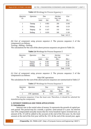
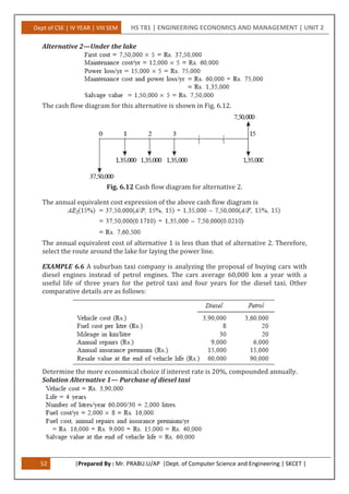
different ways of obtaining the automobile. In either case, the fuel cost and maintenance
cost are borne by the company.
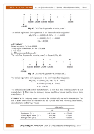
(a) Purchase for cash at Rs. 3,90,000.
(b) Lease a car. The monthly charge is Rs. 10,500 on a 36-month lease payable at
the end of each month. At the end of the three-year period, the car is returned to the
leasing company.
Ramu believes that he should use a 12% interest rate compounded monthly in
determining which alternative to select. If the car could be sold for Rs. 1,20,000 at the
end of the third year, which option should he use to obtain it?
Alternative 1—Purchase car for cash
Purchase price of the car = Rs. 3,90,000
Life = 3 years = 36 months
Salvage value after 3 years = Rs. 1,20,000
Interest rate = 12% (nominal rate, compounded annually)
= 1% compounded monthly
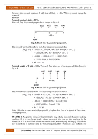
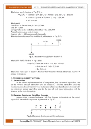
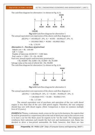
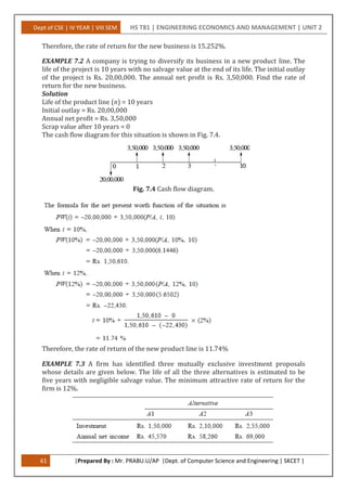
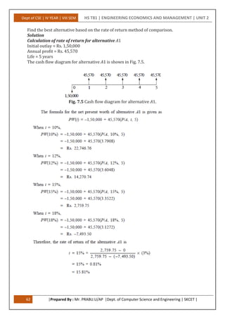
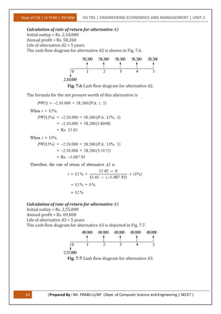
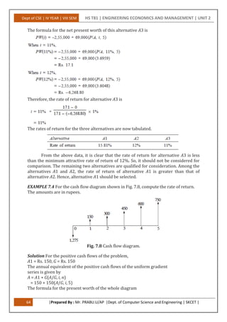
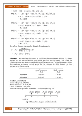
The cash flow diagram for alternative 1 is shown in Fig. 6.15.
Fig. 6.15 Cash flow diagram for alternative 1.
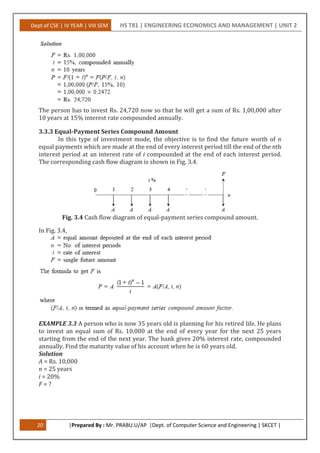
The monthly equivalent cost expression [ME(1%)] of the above cash flow diagram is
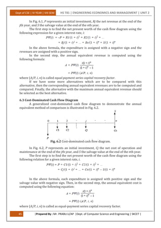
Alternative 2—Use of car under lease
Monthly lease amount for 36 months = Rs. 10,500
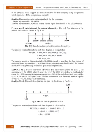
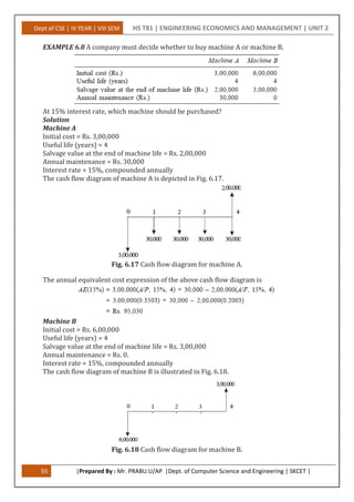
The cash flow diagram for alternative 2 is illustrated in Fig. 6.16.
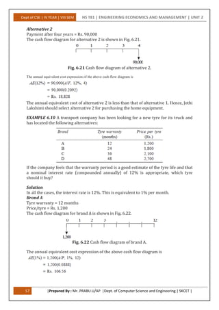
Fig. 6.16 Cash flow diagram for alternative 2.
Monthly equivalent cost = Rs.10,500.
The monthly equivalent cost of alternative 1 is less than that of alternative 2. Hence, the
salesman should purchase the car for cash.](https://image.slidesharecdn.com/unit2-180313055904/85/Elementary-Economic-Analysis-54-320.jpg)

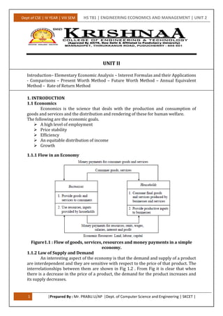
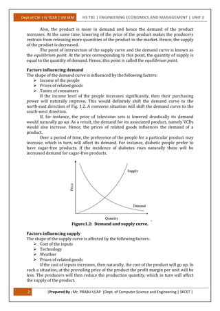
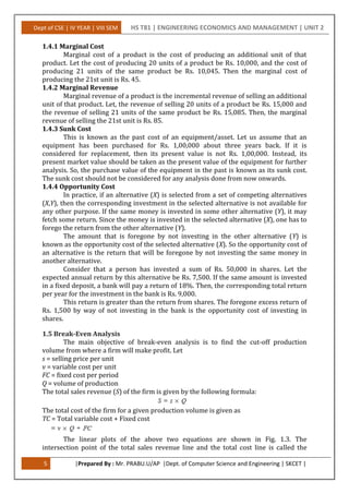
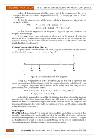
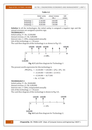
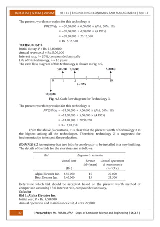
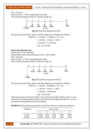
This document provides an overview of engineering economics and elementary economic analysis concepts. It discusses the definition and goals of economics, including the production and distribution of goods and services for human welfare. Key points covered include the law of supply and demand, factors that influence supply and demand, costs and revenues, break-even analysis, and the profit-volume ratio. Elementary economic analysis is introduced as a way to make economic decisions by considering factors like price, transportation costs, availability, and quality when evaluating alternatives. Examples are also provided to illustrate basic economic analysis concepts.


![Microeconomic_Basic_Concepts_&_Principals[1] - Read-Only](https://cdn.slidesharecdn.com/ss_thumbnails/microeconomicbasicconceptsprincipals1-read-only-240514160329-bf7b4dd3-thumbnail.jpg?width=640&height=640&fit=bounds)