Downloaded 138 times


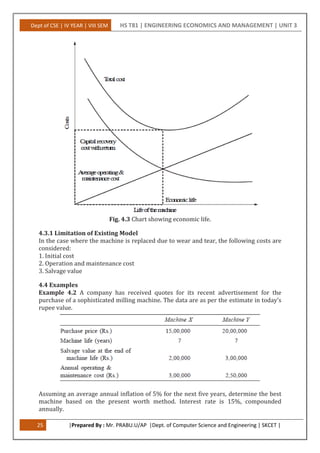
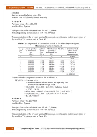
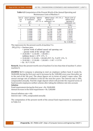

This document discusses replacement and maintenance analysis, including determining the economic life of assets. It provides examples of calculating the economic life of equipment using total cost when interest is 0% and 12%. It also discusses replacement of existing assets, types of maintenance, and a simple probabilistic model for items that fail completely. Optimal replacement policies are determined by comparing individual and group replacement costs. The document also covers several methods of depreciation, including straight-line depreciation calculation examples.