This document defines and describes various fundamental properties of antennas including radiation patterns, field regions, directivity, gain, bandwidth, polarization, input impedance, and the Friis transmission equation. It provides definitions and equations for quantifying properties like radiation intensity, directive gain, directivity, beamwidth, radar cross section, and the radar range equation. Diagrams are included to illustrate concepts such as radiation lobes, coordinate systems, and geometries used in transmission equations.

1. 1
Chapter 2
Fundamental Properties
of Antennas
ECE 5318/6352
Antenna Engineering
Dr. Stuart Long

2. 2

IEEE Standards

Definition of Terms for Antennas

IEEE Standard 145-1983

IEEE Transactions on Antennas and
Propagation Vol. AP-31, No. 6, Part II, Nov. 1983

3. 3

Radiation Pattern
(or Antenna Pattern)
“The spatial distribution of a quantity which
characterizes the electromagnetic field
generated by an antenna.”

4. 4

Distribution can be a

Mathematical function

Graphical representation

Collection of experimental data points

5. 5

Quantity plotted can be a

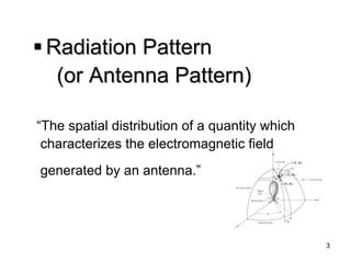
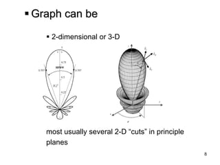
Power flux density W[W/m²]

Radiation intensity U [W/sr]

Field strength E [V/m]

Directivity D

6. 6
 Graph can be

Polar or rectangular

7. 7
 Graph can be

Amplitude field |E| or power |E|² patterns
(in linear scale) (in dB)

8. 8

Graph can be

2-dimensional or 3-D
most usually several 2-D “cuts” in principle
planes

9. 9

Radiation pattern can be

Isotropic
Equal radiation in all directions (not physically realizable, but valuable for comparison purposes)

Directional
Radiates (or receives)
more effectively
in some directions than in others

Omni-directional
nondirectional in azimuth, directional in elevation

10. 10

Principle patterns

E-plane
Plane defined by E-field and direction of maximum radiation

H-plane
Plane defined by H-field and direction of maximum radiation
(usually coincide with principle planes of the coordinate system)

11. 11
Coordinate System
Fig. 2.1 Coordinate system for antenna analysis.

12. 12

Radiation pattern lobes

Major lobe (main beam) in direction of maximum radiation (may be more than one)

Minor lobe - any lobe but a major one

Side lobe - lobe adjacent to major one

Back lobe – minor lobe in direction exactly opposite to major one

13. 13

Side lobe level or ratio (SLR)

(side lobe magnitude / major lobe magnitude)

- 20 dB typical

< -50 dB very difficult
Plot routine included on CD for rectangular and polar graphs

14. 14
Polar Pattern
Fig. 2.3(a) Radiation lobes and
beamwidths of an antenna pattern

15. 15
Linear Pattern
Fig. 2.3(b) Linear plot of power pattern and
its associated lobes and beamwidths

16. 16

Field Regions

Reactive near field
energy stored not radiated
λ= wavelength
D= largest dimension of the antenna
 362.0DR

17. 17

Field Regions

Radiating near field (Fresnel)
radiating fields predominate
pattern still depend on R
radial component may still be appreciable
λ= wavelength
D= largest dimension of the antenna  23262.0DRD

18. 18

Field Regions

Far field (
Fraunhofer Fraunhofer)
field distribution independent of R
field components are essentially transverse  22DR

19. 19

Radian
Fig. 2.10(a) Geometrical arrangements for defining a radian
r
2 radians in full circle
arc length of circle

20. 20

Steradian
one steradian subtends an area of
4π steradians in entire sphere
ddrdAsin2
Fig. 2.10(b) Geometrical arrangements
for defining a steradian.
ddrdAdsin2 2rA

21. 21
 Radiation power density
HEW  

Instantaneous Poynting vector

Time average Poynting vector
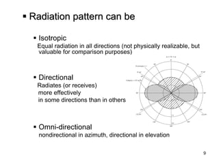
[ W/m ² ]

Total instantaneous
Power

Average radiated
Power
[ W/m ² ]
 ssWP d
[ W ]
HEW  Re21avg  savgraddPsW
[ W ]
[2-8]
[2-9]
[2-4]
[2-3]

22. 22
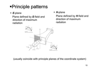
 Radiation intensity
“Power radiated per unit solid angle”
avgWrU2
far zone fields without 1/r factor
22),,( 2),(  rrUE  222),,(),,( 2   rErEr
[W/unit solid angle]
[2-12a]
22oo1(,)(,) 2EE  
Note: This final equation does not have an r in it. The “zero” superscript means that the 1/r term is removed.

23. 23

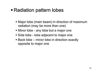
Directive Gain
Ratio of radiation intensity in a given direction to the radiation intensity averaged over all directions
radogPUUUD4

Directivity Gain
(Dg) -- directivity in a given direction
[2-16]
04radPU  
(This is the radiation intensity if the antenna radiated its power equally in all directions.)
201,sin4SUUdd  
Note:

24. 24

Directivity
radmaxomaxoPUUUD4
Do (isotropic) = 1.0
ogDD0

Directivity
-- Do
value of directive gain in direction of maximum radiation intensity

25. 25

Beamwidth

Half power beamwidth
Angle between adjacent points where field strength is 0.707 times the maximum, or the power is 0.5 times the maximum
(-3dB below maximum)

First null beamwidth
Angle between nulls in pattern
Fig. 2.11(b) 2-D power patterns (in linear scale)
of U()=cos²()cos³()

26. 26

Approximate directivity for
omnidirectional patterns

McDonald
2HPBW0027.0HPBW 101  oD
   π
   π

Pozar
(HPBW in degrees)
Results shown with exact values in Fig. 2.18
HPBW1818.01914.172oD nUsin
Better if no minor lobes [2-33b]
[2-32]
[2-33a]
For example

27. 27

Approximate directivity for directional patterns

Kraus
1212441,253orrddD  
   π/2
   π

Tai & Pereira
Antennas with only one narrow main lobe and very negligible minor lobes
22212221815,7218.22ddrroD     nUcos
[2-30b]
[2-31]
[2-27]
For example
( ) HPBW in two perpendicular planes in radians or  in degrees)
12,rr12,dd
Note: According to Elliott, a better number to use in the Kraus formula is 32,400 (Eq. 2-271 in Balanis). In fact, the 41,253 is really wrong (it is derived assuming a rectangular beam footprint instead of the correct elliptical one).

28. 28

Approximate directivity for
directional patterns
Can calculate directivity directly (sect.2.5),
can evaluate directivity numerically (sect. 2.6)
(when integral for Prad cannot be done analytically,
analytical formulas cannot be used )

29. 29

Gain
Like directivity but also takes into account efficiency of antenna
(includes reflection, conductor, and dielectric losses)
 oinoinZZZZ   ;12
eo : overall eff.
er : reflection eff.
ec : conduction eff.
ed : dielectric eff.
Efficiency source) isotropic(lossless,PUPUeDeGinmaxradmaxooooabs 44 dcroeeee dccdeee
[2-49c]
radcdinPeP radoincPeP 

30. 30

Gain
By IEEE definition “gain does not include losses arising from impedance
mismatches (reflection losses) and polarization mismatches (losses)” source) isotropic(lossless,PUDeGinmaxocdo 4
[2-49a]

31. 31

Bandwidth
“frequency range over which some characteristic conforms to a standard”

Pattern bandwidth

Beamwidth, side lobe level, gain, polarization, beam direction

polarization bandwidth example: circular polarization with axial ratio < 3 dB

Impedance bandwidth

usually based on reflection coefficient

under 2 to 1 VSWR typical

32. 32

Bandwidth

Broadband antennas
usually use ratio (e.g. 10:1)

Narrow band antennas
usually use percentage (e.g. 5%)

33. 33

Polarization

Linear

Circular

Elliptical
Right or left handed
rotation in time

34. 34

Polarization

Polarization loss factor

p is angle between wave and antenna polarization
22 ˆˆcoswapPLF
[2-71]

35. 35

Input impedance
“Ratio of voltage to current at terminals of antenna”
ZA = RA + jXA
RA = Rr + RL
Rr = radiation resistance
RL = loss resistance
ZA = antenna impedance at terminals a-b

36. 36

Input impedance

Antenna radiation efficiency
 2221211() 22grrcdrLgrgLIRPowerRadiatedbyAntennaPePowerDeliveredtoAntennaPPIRIR  
[2-90]
LrrcdRRRe  
Note: this works well for those antennas that are modeled as a series RLC circuit – like wire antennas. For those that are modeled as parallel RLC circuit (like a microstrip antenna), we would use G values instead of R values.

37. 37

Friis Transmission Equation
Fig. 2.31 Geometrical orientation of transmitting and receiving antennas for Friis transmission equation

38. 38

Friis Transmission Equation
et = efficiency of transmitting antenna
er = efficiency of receiving antenna
Dt= directive gain of transmitting antenna
Dr = directive gain of receiving antenna
= wavelength
R = distance between antennas
assuming impedance and
polarization matches
224),(),( RDDeePPrrrtttrttr   
[2-117]

39. 39

Radar Range Equation
Fig. 2.32 Geometrical arrangement of
transmitter, target, and receiver for
radar range equation22144),(),(      RRDDeePPrrrttttrcdrcdt    
[2-123]

40. 40

Radar Cross Section
RCS

Usually given symbol 

Far field characteristic

Units in [m²]
4rincUW  incident power density on body from transmit directionincW scattered power intensity in receive directionrU
Physical interpretation: The radar cross section is the area of an equivalent ideal “black body” absorber that absorbs all incident power that then radiates it equally in all directions.

41. 41

Radar Cross Section (
RCS)

Function of

Polarization of the wave

Angle of incidence

Angle of observation

Geometry of target

Electrical properties of target

Frequency

42. 42

Radar Cross Section (
RCS)