This document discusses the concept of diffraction as it relates to wireless communication. It explains that diffraction allows radio signals to propagate behind obstacles between a transmitter and receiver. It presents Huygen's principle, which states that each point on a wavefront can be considered a secondary source of wavelets. These wavelets combine to form a new wavefront. The document also covers knife-edge diffraction geometry and how to calculate the excess path length and phase difference between the diffracted and direct paths. It defines Fresnel zones and introduces the Fresnel zone diffraction parameter used to determine whether interference will be constructive or destructive. Additionally, it explains diffraction loss that occurs when secondary waves are blocked, resulting in only partial energy being diffract

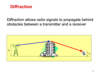
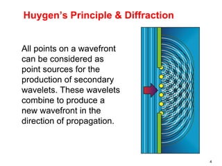
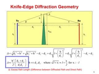
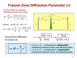
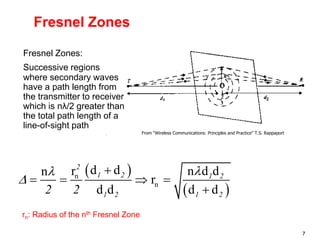
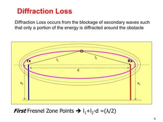
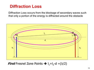
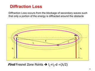
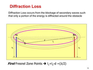
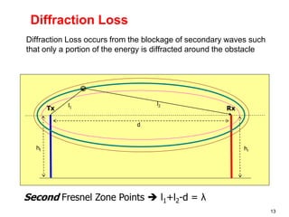
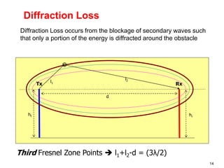
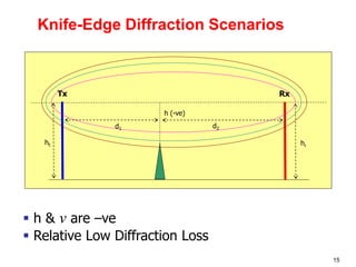
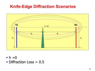
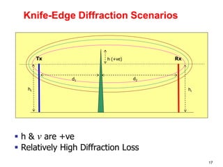
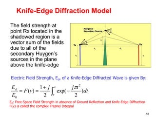
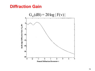
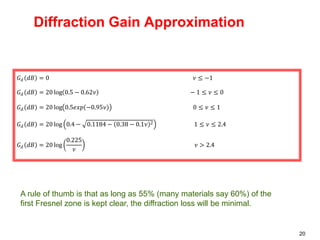
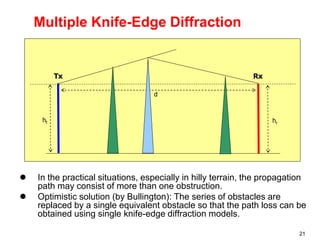
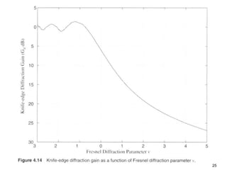
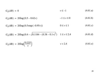
1. Wireless Communication
Channels: Large-Scale Pathloss

2. Diffraction

3. 3
Diffraction
Diffraction allows radio signals to propagate behind
obstacles between a transmitter and a receiver
ht
hr

4. 4
Huygen’s Principle & Diffraction
All points on a wavefront
can be considered as
point sources for the
production of secondary
wavelets. These wavelets
combine to produce a
new wavefront in the
direction of propagation.

5. 5
Knife-Edge Diffraction Geometry
ht hr
d1 d2
hobs
h
Tx Rx
α
β γ
Δ: Excess Path Length (Difference between Diffracted Path and Direct Path)
h h
d h d h d d d d d d
d d
d d
h x
h d d where x for x
d d
2 2
2 2 2 2
1 2 1 2 1 2 1 2
1 2
2
1 2
1 2
1 2
1 1
, 1 1 1
2 2


   
           
   
   
 

    
 
 
<
<

6. 6
Ф: Phase Difference between
Diffracted Path and Direct Path)
d d
h
d d
2
1 2
1 2
2 2
2
 
 
 
 

   
 
 
Assume
h d d
h h
d d d d
1 2
1 2 1 2
tan tan
   
  
 

     
 
 
d d d d
h
d d d d
1 2 1 2
1 2 1 2
2 2
 
 

 

Fresnel Zone Diffraction
Parameter (ν)
Fresnel Zone Diffraction Parameter (ν)
2
2

 
 
 ν2=2, 6, 10 … corresponds to destructive
interference between direct and diffracted paths
 ν2=4, 8, 12 … corresponds to constructive
interference between direct and diffracted paths

7. 7
Fresnel Zones
From “Wireless Communications: Principles and Practice” T.S. Rappaport
Fresnel Zones:
Successive regions
where secondary waves
have a path length from
the transmitter to receiver
which is nλ/2 greater than
the total path length of a
line-of-sight path
 
 
n
n
d d
r n d d
n
r
d d d d
2
1 2 1 2
1 2 1 2
2 2




   

rn: Radius of the nth Fresnel Zone

8. 8
Diffraction Loss
Diffraction Loss occurs from the blockage of secondary waves such
that only a portion of the energy is diffracted around the obstacle
ht hr
Tx Rx
l1
l2
d
First Fresnel Zone Points  l1+l2-d =(λ/2)

9. 9
Diffraction Loss
Diffraction Loss occurs from the blockage of secondary waves such
that only a portion of the energy is diffracted around the obstacle
ht hr
Tx Rx
l1
l2
d
First Fresnel Zone Points  l1+l2-d =(λ/2)

10. 10
Diffraction Loss
Diffraction Loss occurs from the blockage of secondary waves such
that only a portion of the energy is diffracted around the obstacle
ht hr
Tx Rx
l1
l2
d
First Fresnel Zone Points  l1+l2-d =(λ/2)

11. 11
Diffraction Loss
Diffraction Loss occurs from the blockage of secondary waves such
that only a portion of the energy is diffracted around the obstacle
ht hr
Tx Rx
l1
l2
d
First Fresnel Zone Points  l1+l2-d =(λ/2)

12. 12
Diffraction Loss
Diffraction Loss occurs from the blockage of secondary waves such
that only a portion of the energy is diffracted around the obstacle
ht hr
Tx Rx
l1 l2
d
First Fresnel Zone Points  l1+l2-d =(λ/2)

13. 13
Diffraction Loss
Diffraction Loss occurs from the blockage of secondary waves such
that only a portion of the energy is diffracted around the obstacle
ht hr
Tx Rx
l1
l2
d
Second Fresnel Zone Points  l1+l2-d = λ

14. 14
Diffraction Loss
Diffraction Loss occurs from the blockage of secondary waves such
that only a portion of the energy is diffracted around the obstacle
ht hr
Tx Rx
l1
l2
d
Third Fresnel Zone Points  l1+l2-d = (3λ/2)

15. 15
Knife-Edge Diffraction Scenarios
ht hr
Tx Rx
d1 d2
h (-ve)
 h & ν are –ve
 Relative Low Diffraction Loss

16. 16
ht hr
Tx Rx
d1 d2
h =0
Knife-Edge Diffraction Scenarios
 h =0
 Diffraction Loss = 0.5

17. 17
Knife-Edge Diffraction Scenarios
ht hr
Tx Rx
d1 d2
h (+ve)
 h & ν are +ve
 Relatively High Diffraction Loss

18. 18
Knife-Edge Diffraction Model
The field strength at
point Rx located in the
shadowed region is a
vector sum of the fields
due to all of the
secondary Huygen’s
sources in the plane
above the knife-edge
Electric Field Strength, Ed, of a Knife-Edge Diffracted Wave is given By:
E0: Free-Space Field Strength in absence of Ground Reflection and Knife-Edge Diffraction
F(ν) is called the complex Fresnel Integral

19. 19
Diffraction Gain

20. 20
Diffraction Gain Approximation
𝐺𝑑 𝑑𝐵 = 0 𝜈 ≤ −1
𝐺𝑑 𝑑𝐵 = 20 log 0.5 − 0.62𝜈 − 1 ≤ 𝜈 ≤ 0
𝐺𝑑 𝑑𝐵 = 20 log 0.5𝑒𝑥𝑝 −0.95𝜈 0 ≤ 𝜈 ≤ 1
𝐺𝑑 𝑑𝐵 = 20 log 0.4 − 0.1184 − 0.38 − 0.1𝜈 2 1 ≤ 𝜈 ≤ 2.4
𝐺𝑑 𝑑𝐵 = 20 log
0.225
𝜈
𝜈 > 2.4
A rule of thumb is that as long as 55% (many materials say 60%) of the
first Fresnel zone is kept clear, the diffraction loss will be minimal.

21. 21
Multiple Knife-Edge Diffraction
ht hr
Tx Rx
d
 In the practical situations, especially in hilly terrain, the propagation
path may consist of more than one obstruction.
 Optimistic solution (by Bullington): The series of obstacles are
replaced by a single equivalent obstacle so that the path loss can be
obtained using single knife-edge diffraction models.

22. 22

23. 23

24. 24

25. 25

26. 26