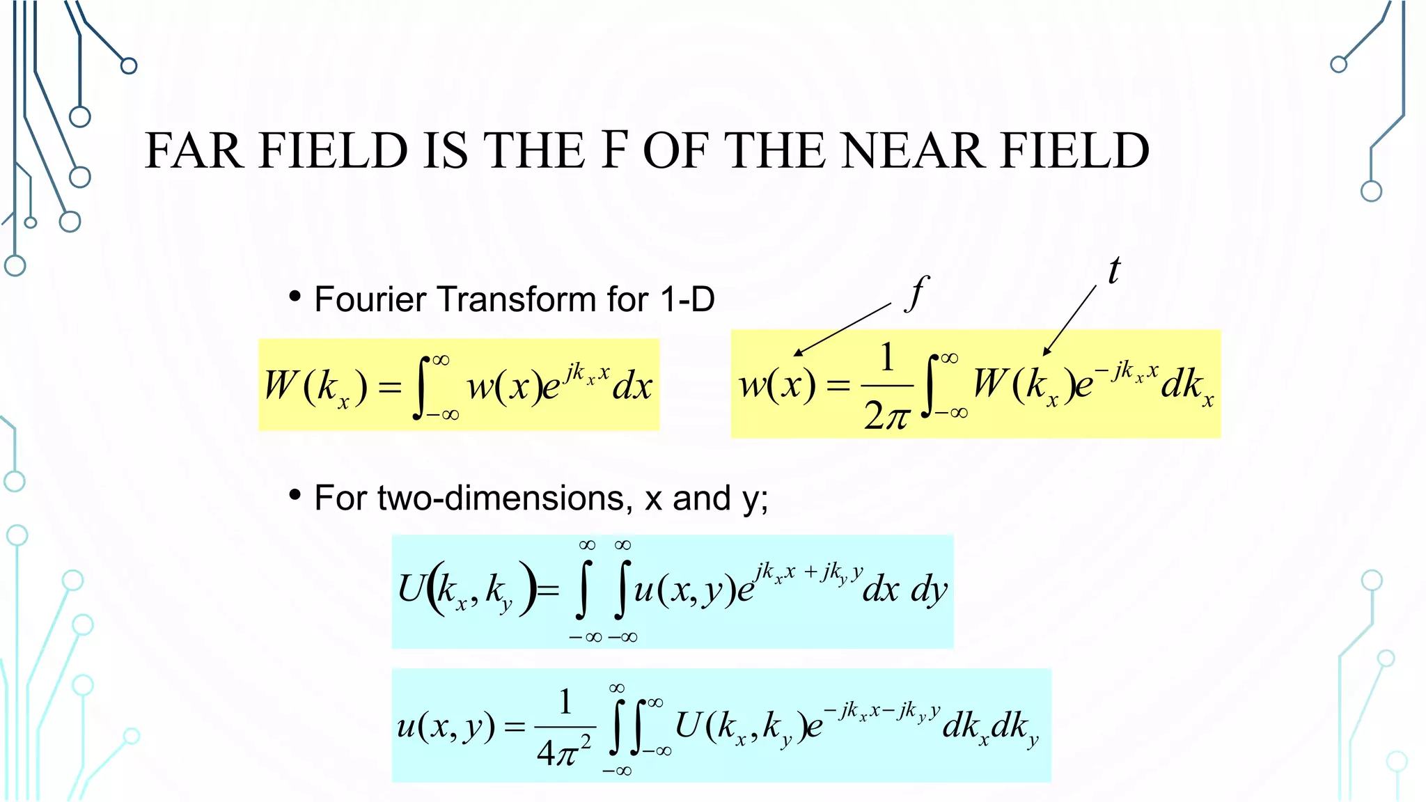
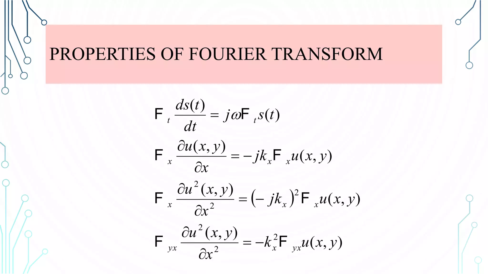
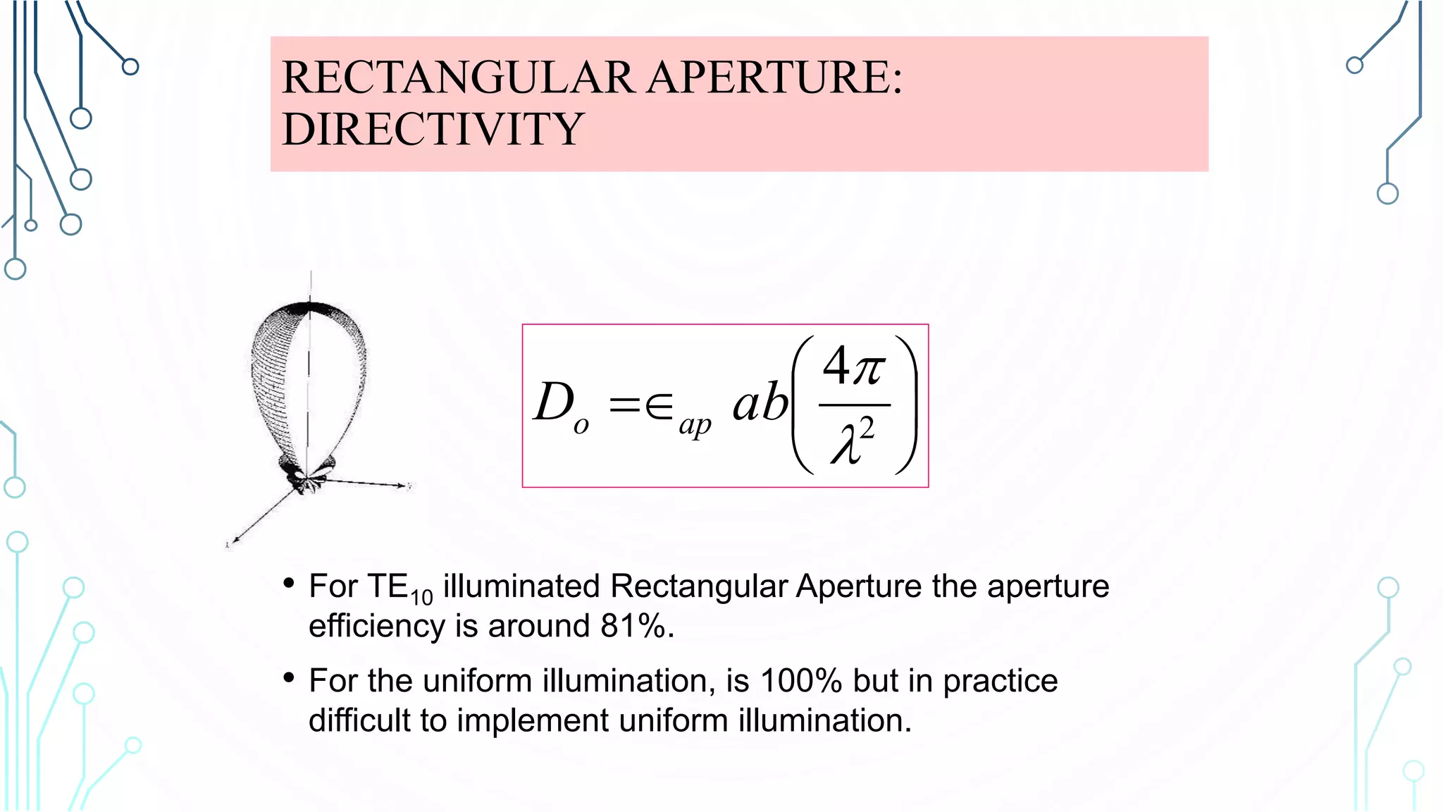
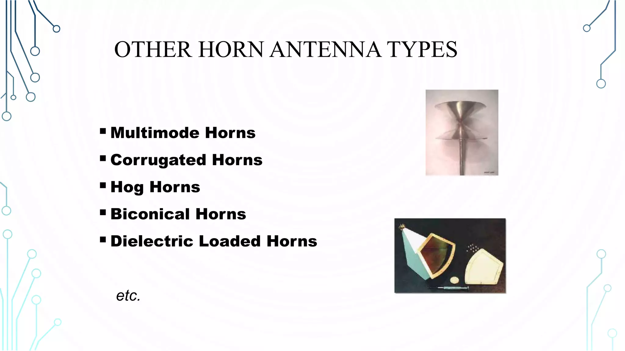
APERTURE AND HORN
ANTENNA
OUTLINE
1)Aperture Antenna
a) Huygen’s Principle
b) Radiation Pattern
c) Directivity
d) Rectangular Apertures
e) Circular Apertures
2)Horn Antenna
a) E Plane Sectoral Horn
b) H Plane Sectoral Horn
c) Pyramidal Horn
d) Conical Horn
e) Other types of Horn Antenna
3) Application
APERTURE ANTENNA
•Most common at microwave frequencies (300MHz-
300GHz)
•They may take the form of a waveguide or a horn
whose aperture may be square, rectangular, circular,
elliptical, or any other configuration.
•We will analyze radiation characteristics at far field
• Rectangular Aperture
• Circular Aperture
FIELD EQUIVALENCE PRINCIPLE:
HUYGEN’S PRINCIPLE
• Introduced in1936 by A. Schelkunoff, which is a more
rigorous formulation of Huygen’s Principle which states that
“Every point on a wave-front may be considered a source of
secondary spherical wavelets which spread out in the
forward direction at the speed of light. The new wave-front
is the tangential surface to all of these secondary wavelets.”
• A principle by which actual sources, such as antenna and
transmitter, are replaced by equivalent source.
FIELD EQUIVALENCE PRINCIPLE:
HUYGEN’S PRINCIPLE
FIELD EQUIVALENCE PRINCIPLE:
HUYGEN’S PRINCIPLE
• The Huygen’s principle is based on the uniqueness theorem
which states that “a field in a lossy region is uniquely
specified by the sources within the region plus the
tangential components of the electric field over the
boundary, or the tangential components of the magnetic
field over the boundary, or the former over part of the
boundary and the latter over the rest of the boundary.”
FAR FIELD IS THE F OF THE NEAR FIELD
• Fourier Transform for 1-D
• For two-dimensions, x and y;
dxexwkW xjk
x
x



 )()( x
xjk
x dkekWxw x
 )(
2
1
)(

f
t
U kx, ky  u(x, y)e
jkxx  jky y




 dx dy





 yx
yjkxjk
yx dkdkekkUyxu yx
),(
4
1
),( 2

PROPERTIES OF FOURIER TRANSFORM
 
),(
),(
),(
),(
),(
),(
)(
)(
2
2
2
2
2
2
yxuk
x
yxu
yxujk
x
yxu
yxujk
x
yxu
tsj
dt
tds
yxxyx
xxx
xxx
tt
FF
FF
FF
FF









 
0
022


E
EE ok
0
),,(),,(),,(
02
2
2
2
2
2
2




























z
zyxE
y
zyxE
x
zyxE
k
zyx
zyx
o EE
Taking the Fourier transform of the 2 equations above:
0
),,(
),,(),,(
0),,()(),,( 222
2
2












z
zkkE
jzkkEkzkkEk
zkkkkkzkk
z
yxz
yxyyyxxx
yxyxoyx EE
Now, we define,
And we obtain,
Which has a solution of
Then we take the inverse transform
2222
yxoz kkkk 
0),,(
),,( 2
2
2



zkkk
z
zkk
yxz
yx
E
E
zjk
yxyx
z
ekkzkk 
 ),(),,( fE






 yx
j
yx dkdkekkzyx rk
fE ),(
4
1
),,( 2

If z=0, then, we are at the aperture
Which looks like:
Which is the inverse of F…





 yx
yjkxjk
yxa dkdkekkyxyx yx
),(
4
1
)0,,(),( 2tan fEE






 yx
yjkxjk
yx dkdkekkUyxu yx
),(
4
1
),( 2

This is the Fourier transform for 2 dimensions, so:
dxdyeyxEkk
yjkxjk
a
S
yxt
yx
a

 ),(),(f
 


sinsin,coscos
2
cos
)( bkake
r
jk
r oot
rjko o
fE 

U kx, ky  u(x, y)e
jkxx  jky y




 dx dy
Therefore, if we know the field at the aperture, we can
used these equations to find E(r).
=>First, we’ll look at the case when the illumination at
the rectangular aperture it’s uniform.
It can be shown that,
UNIFORMLY ILLUMINATED
RECTANGULAR APERTURE
elsewhere0
for),(

 b|y|a|x|Eyx oa xE
dxdyeE
yjkxjk
a
a
b
b
ot
yx 
 
  xf
   
v
v
u
u
abE
bk
bk
ak
ak
abE
bk
bk
ak
ak
abE
o
o
o
o
o
o
y
y
x
x
o
sinsin
4
sinsin
sinsinsin
cossin
cossinsin
4
sinsin
4
x
x
x







 

coscosˆsinˆsinsin
2
4
)( φθE  
v
v
u
u
e
r
abEjk
r rjkoo o
HOW DOES THIS PATTERN LOOKS…


sinsin
cossin
bkv
aku
o
o


In this report we considered TE10 and TE11
mode for illuminated rectangular aperture.
TE10 ILLUMINATED RECTANGULAR
APERTURE
elsewhere0
2/'2/-
2/'2/-
forˆ
'
cos),(










byb
axa
y
a
x
Eyx oa

E
dxdye
a
x
yE
yjkxjk
a
a
b
b
ot
yx 
 
  )(cosˆ

f


sinsin
2
cossin
2
bkv
v
Y
aku
u
X
o
o


 

coscosˆsinˆsin
2
cos
4
)( 2
2
φθE 










Y
Y
X
X
r
eabEjk
r
rjk
oo
o
RECTANGULAR APERTURE:
DIRECTIVITY
• For TE10 illuminated Rectangular Aperture the aperture
efficiency is around 81%.
• For the uniform illumination, is 100% but in practice
difficult to implement uniform illumination.






 2
4


abD apo
CIRCULAR
APERTURE
(Uniform illumination)
• In this case we use cylindrical coordinates


ddeE ojk
a
ot ')'cos(sin
0
2
0

  xf
 



sin
sin
2 12
ak
akJ
Ea
o
o
ox
CIRCULAR APERTURE W/ UNIFORM
ILLUMINATION
• For TE11 illuminated Circular Aperture the aperture
efficiency is around 84%.
• For the uniform illumination, is 100% but in practice
difficult to implement uniformity
2








C
D apo
flared waveguides that produce a nearly uniform
phase front larger than the waveguide itself
constructed in a variety of shapes such as
sectoral E-plane, sectoral H-plane, pyramidal,
conical, etc.
HORN ANTENNA
RADIATION PATTERN
APPLICATION AREAS
used as a feed element for large radio astronomy,
satellite tracking and communication dishes
A common element of phased arrays
used in the calibration, other high-gain antennas
used for making electromagnetic interference
measurements
E-PLANE SECTORAL HORN
Fields expressions OVER THE horn are similar to the
fields of a TE10 mode for a rectangular waveguide with
the aperture dimensions of a and b1.
difference is in the complex exponential term,
parabolic phase error,.
 )2/(
1
1
2
cos),(  ykj
y ex
a
EyxE 







 )2/(
1
1
2
sin),( 

 ykj
z ex
aka
jEyxH 













 )2/(1 1
2
cos),( 

ykj
x ex
a
E
yxH 







• this is the plane containing the magnetic field vector
(sometimes called the H aperture) and the direction of
maximum radiation
H-PLANE SECTORAL HORN
PYRAMIDAL HORN
combination of the E-plane and H-plane
horns and as such is flared in both
directions
CONICAL HORN ANTENNA:
A horn in the shape of a cone , with a circular
cross section. They are used with cylindrical
waveguides.
0
0
0
30
0
60
0
90
0
120
0
150
0
180
0
150
0
120
0
90
0
60
0
30
102030
10
20
30
Relativepower(dBdown)
E- and H-Plane Patterns of
the E-Plane Sectoral Horn
E-Plane
H-Plane
E- and H-Plane Patterns of
the H-Plane Sectoral Horn
E-Plane
H-Plane
0
0
0
30
0
60
0
90
0
120
0
150
0
180
0
150
0
120
0
90
0
60
0
30
102030
10
20
30
Relativepower(dBdown)
E and H-Plane Patterns
E-Plane
H-Plane
0
0
0
30
0
60
0
90
0
120
0
150
0
180
0
150
0
120
0
90
0
60
0
30
102030
10
20
30
Relativepower(dBdown)
E- and H-Plane Patterns of
The Conical Horn Antenna
E-Plane
H-Plane
0
0
0
30
0
60
0
90
0
120
0
150
0
180
0
150
0
120
0
90
0
60
0
30
102030
10
20
30
Relativepower(dBdown)
DIRECTIVITY:
• Directivity of an E-plane sectored horn is:
𝐷 𝐸 =
4𝜋𝑈𝑚𝑎𝑥
𝑃 𝑟𝑎𝑑
=
64𝑎𝜌1
𝜋𝜆𝑏1
𝑐2 𝑏1
2𝜆𝜌1
+𝑠2 𝑏1
2𝜆𝜌1
• Directivity of an H-plane sectored horn is:
𝐷 𝐻 =
4𝜋𝑏𝜌2
𝑎1 𝜆
𝑐 𝑢 − 𝑐 𝑣 2 + 𝑠 𝑢 − 𝑠 𝑣 2
where 𝜌1 = 𝜌e cos 𝜑 𝑒
c(u),c(v),s(u) & s(v) are Fresnel integrals
a & b are dimensions of wave guide
DIRECTIVITY:
• Directivity of a pyramidal horn antenna is:
𝐷 𝐻 =
𝜋𝜆2
32𝑎𝑏
𝐷 𝐸 ∗ 𝐷𝐻
where D 𝐻 = Directivity of an H−plane sectored horn
DE= Directivity of an E-plane sectored horn
a & b are dimensions of wave guide
OTHER HORN ANTENNA TYPES
Multimode Horns
Corrugated Horns
Hog Horns
Biconical Horns
Dielectric Loaded Horns
etc.
APPLICATIONS:
• In satellite
communication
• In TV base station
Large 177 ft. horn reflector
antenna at AT&T satellite
communication facility in
Andover, Maine, USA.
HORN ANTENNA IN A DISH ANTENNA:
HORN ANTENNA IN SHORT RANGE
RADARS:

Apperture and Horn Antenna

  • 1.
  • 2.
    OUTLINE 1)Aperture Antenna a) Huygen’sPrinciple b) Radiation Pattern c) Directivity d) Rectangular Apertures e) Circular Apertures 2)Horn Antenna a) E Plane Sectoral Horn b) H Plane Sectoral Horn c) Pyramidal Horn d) Conical Horn e) Other types of Horn Antenna 3) Application
  • 3.
    APERTURE ANTENNA •Most commonat microwave frequencies (300MHz- 300GHz) •They may take the form of a waveguide or a horn whose aperture may be square, rectangular, circular, elliptical, or any other configuration. •We will analyze radiation characteristics at far field • Rectangular Aperture • Circular Aperture
  • 4.
    FIELD EQUIVALENCE PRINCIPLE: HUYGEN’SPRINCIPLE • Introduced in1936 by A. Schelkunoff, which is a more rigorous formulation of Huygen’s Principle which states that “Every point on a wave-front may be considered a source of secondary spherical wavelets which spread out in the forward direction at the speed of light. The new wave-front is the tangential surface to all of these secondary wavelets.” • A principle by which actual sources, such as antenna and transmitter, are replaced by equivalent source.
  • 5.
  • 6.
    FIELD EQUIVALENCE PRINCIPLE: HUYGEN’SPRINCIPLE • The Huygen’s principle is based on the uniqueness theorem which states that “a field in a lossy region is uniquely specified by the sources within the region plus the tangential components of the electric field over the boundary, or the tangential components of the magnetic field over the boundary, or the former over part of the boundary and the latter over the rest of the boundary.”
  • 7.
    FAR FIELD ISTHE F OF THE NEAR FIELD • Fourier Transform for 1-D • For two-dimensions, x and y; dxexwkW xjk x x     )()( x xjk x dkekWxw x  )( 2 1 )(  f t U kx, ky  u(x, y)e jkxx  jky y      dx dy       yx yjkxjk yx dkdkekkUyxu yx ),( 4 1 ),( 2 
  • 8.
    PROPERTIES OF FOURIERTRANSFORM   ),( ),( ),( ),( ),( ),( )( )( 2 2 2 2 2 2 yxuk x yxu yxujk x yxu yxujk x yxu tsj dt tds yxxyx xxx xxx tt FF FF FF FF           
  • 9.
    0 022   E EE ok 0 ),,(),,(),,( 02 2 2 2 2 2 2                             z zyxE y zyxE x zyxE k zyx zyx o EE Takingthe Fourier transform of the 2 equations above: 0 ),,( ),,(),,( 0),,()(),,( 222 2 2             z zkkE jzkkEkzkkEk zkkkkkzkk z yxz yxyyyxxx yxyxoyx EE
  • 10.
    Now, we define, Andwe obtain, Which has a solution of Then we take the inverse transform 2222 yxoz kkkk  0),,( ),,( 2 2 2    zkkk z zkk yxz yx E E zjk yxyx z ekkzkk   ),(),,( fE        yx j yx dkdkekkzyx rk fE ),( 4 1 ),,( 2 
  • 11.
    If z=0, then,we are at the aperture Which looks like: Which is the inverse of F…       yx yjkxjk yxa dkdkekkyxyx yx ),( 4 1 )0,,(),( 2tan fEE        yx yjkxjk yx dkdkekkUyxu yx ),( 4 1 ),( 2 
  • 12.
    This is theFourier transform for 2 dimensions, so: dxdyeyxEkk yjkxjk a S yxt yx a   ),(),(f     sinsin,coscos 2 cos )( bkake r jk r oot rjko o fE   U kx, ky  u(x, y)e jkxx  jky y      dx dy Therefore, if we know the field at the aperture, we can used these equations to find E(r). =>First, we’ll look at the case when the illumination at the rectangular aperture it’s uniform. It can be shown that,
  • 13.
    UNIFORMLY ILLUMINATED RECTANGULAR APERTURE elsewhere0 for),(  b|y|a|x|Eyx oa xE dxdyeE yjkxjk a a b b ot yx      xf     v v u u abE bk bk ak ak abE bk bk ak ak abE o o o o o o y y x x o sinsin 4 sinsin sinsinsin cossin cossinsin 4 sinsin 4 x x x           coscosˆsinˆsinsin 2 4 )( φθE   v v u u e r abEjk r rjkoo o
  • 14.
    HOW DOES THISPATTERN LOOKS…   sinsin cossin bkv aku o o  
  • 15.
    In this reportwe considered TE10 and TE11 mode for illuminated rectangular aperture.
  • 16.
    TE10 ILLUMINATED RECTANGULAR APERTURE elsewhere0 2/'2/- 2/'2/- forˆ ' cos),(           byb axa y a x Eyxoa  E dxdye a x yE yjkxjk a a b b ot yx      )(cosˆ  f   sinsin 2 cossin 2 bkv v Y aku u X o o      coscosˆsinˆsin 2 cos 4 )( 2 2 φθE            Y Y X X r eabEjk r rjk oo o
  • 17.
    RECTANGULAR APERTURE: DIRECTIVITY • ForTE10 illuminated Rectangular Aperture the aperture efficiency is around 81%. • For the uniform illumination, is 100% but in practice difficult to implement uniform illumination.        2 4   abD apo
  • 18.
    CIRCULAR APERTURE (Uniform illumination) • Inthis case we use cylindrical coordinates   ddeE ojk a ot ')'cos(sin 0 2 0    xf      sin sin 2 12 ak akJ Ea o o ox
  • 19.
    CIRCULAR APERTURE W/UNIFORM ILLUMINATION • For TE11 illuminated Circular Aperture the aperture efficiency is around 84%. • For the uniform illumination, is 100% but in practice difficult to implement uniformity 2         C D apo
  • 20.
    flared waveguides thatproduce a nearly uniform phase front larger than the waveguide itself constructed in a variety of shapes such as sectoral E-plane, sectoral H-plane, pyramidal, conical, etc. HORN ANTENNA
  • 21.
  • 22.
    APPLICATION AREAS used asa feed element for large radio astronomy, satellite tracking and communication dishes A common element of phased arrays used in the calibration, other high-gain antennas used for making electromagnetic interference measurements
  • 23.
    E-PLANE SECTORAL HORN Fieldsexpressions OVER THE horn are similar to the fields of a TE10 mode for a rectangular waveguide with the aperture dimensions of a and b1. difference is in the complex exponential term, parabolic phase error,.  )2/( 1 1 2 cos),(  ykj y ex a EyxE          )2/( 1 1 2 sin),(    ykj z ex aka jEyxH                )2/(1 1 2 cos),(   ykj x ex a E yxH        
  • 24.
    • this isthe plane containing the magnetic field vector (sometimes called the H aperture) and the direction of maximum radiation H-PLANE SECTORAL HORN
  • 25.
    PYRAMIDAL HORN combination ofthe E-plane and H-plane horns and as such is flared in both directions
  • 26.
    CONICAL HORN ANTENNA: Ahorn in the shape of a cone , with a circular cross section. They are used with cylindrical waveguides.
  • 27.
  • 28.
    E- and H-PlanePatterns of the H-Plane Sectoral Horn E-Plane H-Plane 0 0 0 30 0 60 0 90 0 120 0 150 0 180 0 150 0 120 0 90 0 60 0 30 102030 10 20 30 Relativepower(dBdown)
  • 29.
    E and H-PlanePatterns E-Plane H-Plane 0 0 0 30 0 60 0 90 0 120 0 150 0 180 0 150 0 120 0 90 0 60 0 30 102030 10 20 30 Relativepower(dBdown)
  • 30.
    E- and H-PlanePatterns of The Conical Horn Antenna E-Plane H-Plane 0 0 0 30 0 60 0 90 0 120 0 150 0 180 0 150 0 120 0 90 0 60 0 30 102030 10 20 30 Relativepower(dBdown)
  • 31.
    DIRECTIVITY: • Directivity ofan E-plane sectored horn is: 𝐷 𝐸 = 4𝜋𝑈𝑚𝑎𝑥 𝑃 𝑟𝑎𝑑 = 64𝑎𝜌1 𝜋𝜆𝑏1 𝑐2 𝑏1 2𝜆𝜌1 +𝑠2 𝑏1 2𝜆𝜌1 • Directivity of an H-plane sectored horn is: 𝐷 𝐻 = 4𝜋𝑏𝜌2 𝑎1 𝜆 𝑐 𝑢 − 𝑐 𝑣 2 + 𝑠 𝑢 − 𝑠 𝑣 2 where 𝜌1 = 𝜌e cos 𝜑 𝑒 c(u),c(v),s(u) & s(v) are Fresnel integrals a & b are dimensions of wave guide
  • 32.
    DIRECTIVITY: • Directivity ofa pyramidal horn antenna is: 𝐷 𝐻 = 𝜋𝜆2 32𝑎𝑏 𝐷 𝐸 ∗ 𝐷𝐻 where D 𝐻 = Directivity of an H−plane sectored horn DE= Directivity of an E-plane sectored horn a & b are dimensions of wave guide
  • 33.
    OTHER HORN ANTENNATYPES Multimode Horns Corrugated Horns Hog Horns Biconical Horns Dielectric Loaded Horns etc.
  • 34.
    APPLICATIONS: • In satellite communication •In TV base station Large 177 ft. horn reflector antenna at AT&T satellite communication facility in Andover, Maine, USA.
  • 35.
    HORN ANTENNA INA DISH ANTENNA:
  • 36.
    HORN ANTENNA INSHORT RANGE RADARS: