The document discusses adaptive filters, highlighting their time-varying characteristics and how they differ from fixed FIR and IIR filters. It details the structure of adaptive filters, their algorithms, and applications in system identification, adaptive prediction, and noise cancellation. MATLAB tools for designing adaptive filters and examples illustrating their implementation and performance are also provided.
![© M.S Ramaiah School of Advanced Studies - Bangalore 9
PEPs- ESD 521
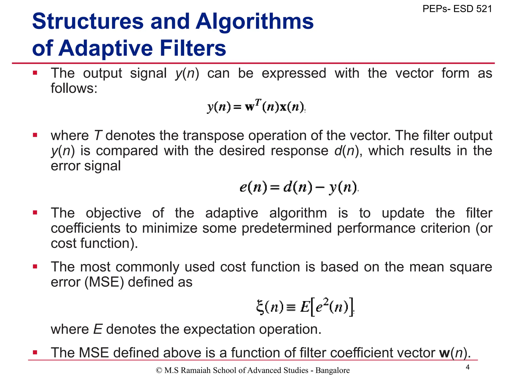
Case Study Example 4.9
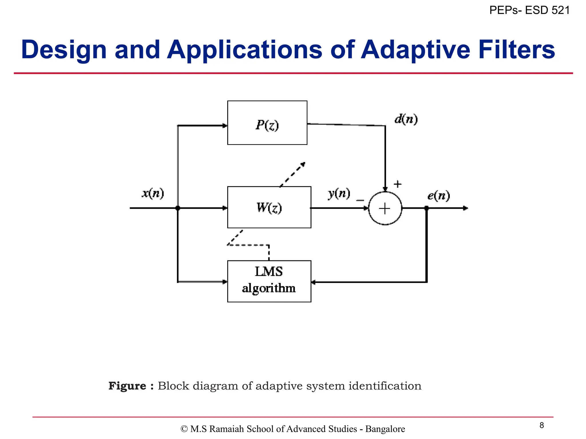
In the figure, an unknown system P(z) is an FIR filter designed by
the following function:
p = fir1(15,0.5);
The excitation signal x(n) used for system identification is generated
as follows:
x = randn(1,400);
Use an adapting filter W(z) with the LMS algorithm to identify P(z).
The length of the adaptive filter is 16, and the step size is 0.01. The
adaptive filtering is conducted as follows:
ha = adaptfilt.lms(16,mu);
[y,e] = filter(ha,x,d);](https://image.slidesharecdn.com/adaptivefilters-231010073507-2e0fafed/75/Adaptive-Filters-ppt-9-2048.jpg)
![© M.S Ramaiah School of Advanced Studies - Bangalore 10
PEPs- ESD 521
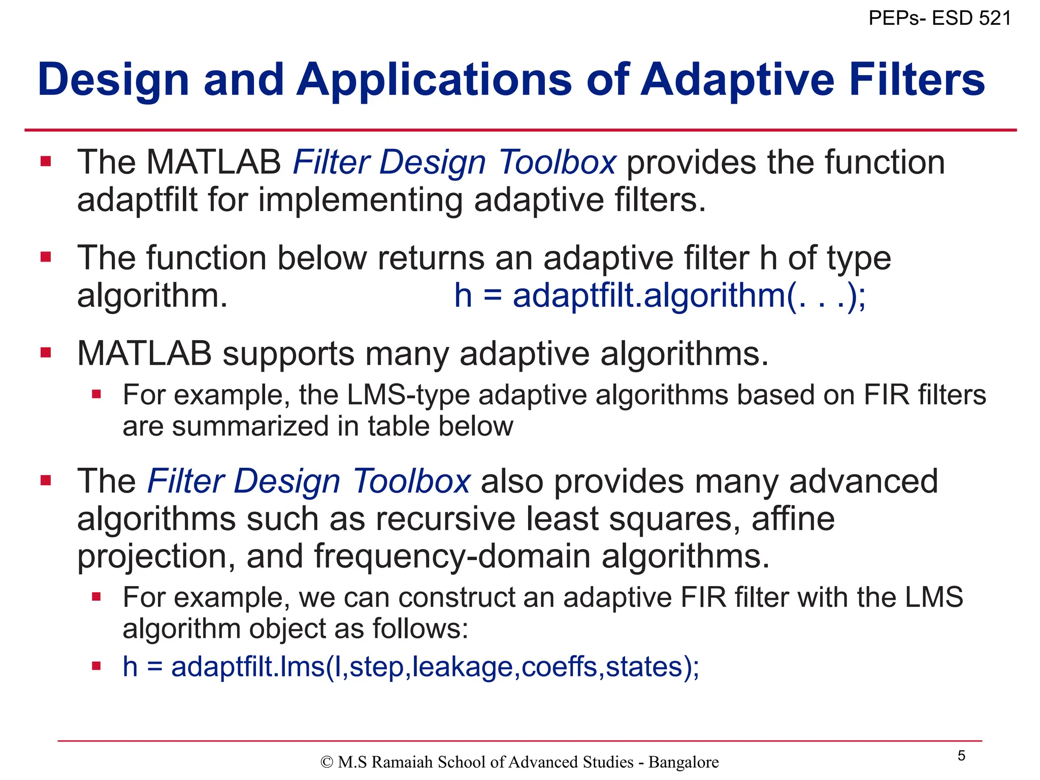
Case Study Example 4.9
% Example 4.9
% Description: Adaptive system identification of unknown system P(z), which is an FIR filter
x = randn(1,400); % excitation signal x(n)
p = fir1(15,0.5); % FIR P(z) to be identified
d = filter(p,1,x); % FIR filtering x(n) by P(z)
% to obtain desired signal d(n)
mu = 0.01; % step size mu
ha = adaptfilt.lms(16,mu); % construct adaptive filter object
[y,e] = filter(ha,x,d); % adaptive filtering to get y(n) and e(n)
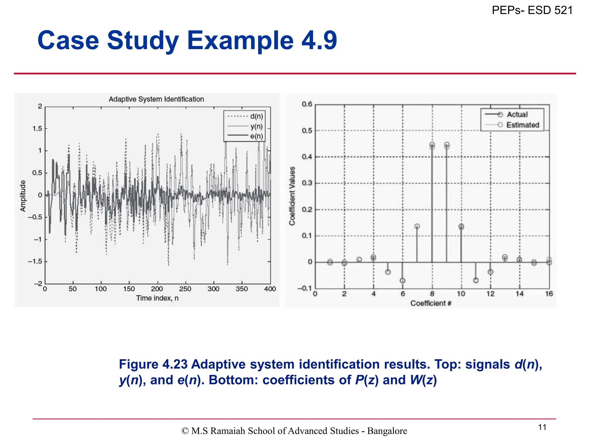
plot(1:400,[d;y;e]);
title('Adaptive System Identification');
legend('d(n)','y(n)','e(n)');
xlabel('Time index, n'); ylabel('Amplitude');
pause;
title('Adaptive System Identification');
stem([p.',ha.coefficients.']);
legend('Actual','Estimated');
xlabel('Coefficient #'); ylabel('Coefficient Values'); grid on;](https://image.slidesharecdn.com/adaptivefilters-231010073507-2e0fafed/75/Adaptive-Filters-ppt-10-2048.jpg)


![© M.S Ramaiah School of Advanced Studies - Bangalore 16
PEPs- ESD 521
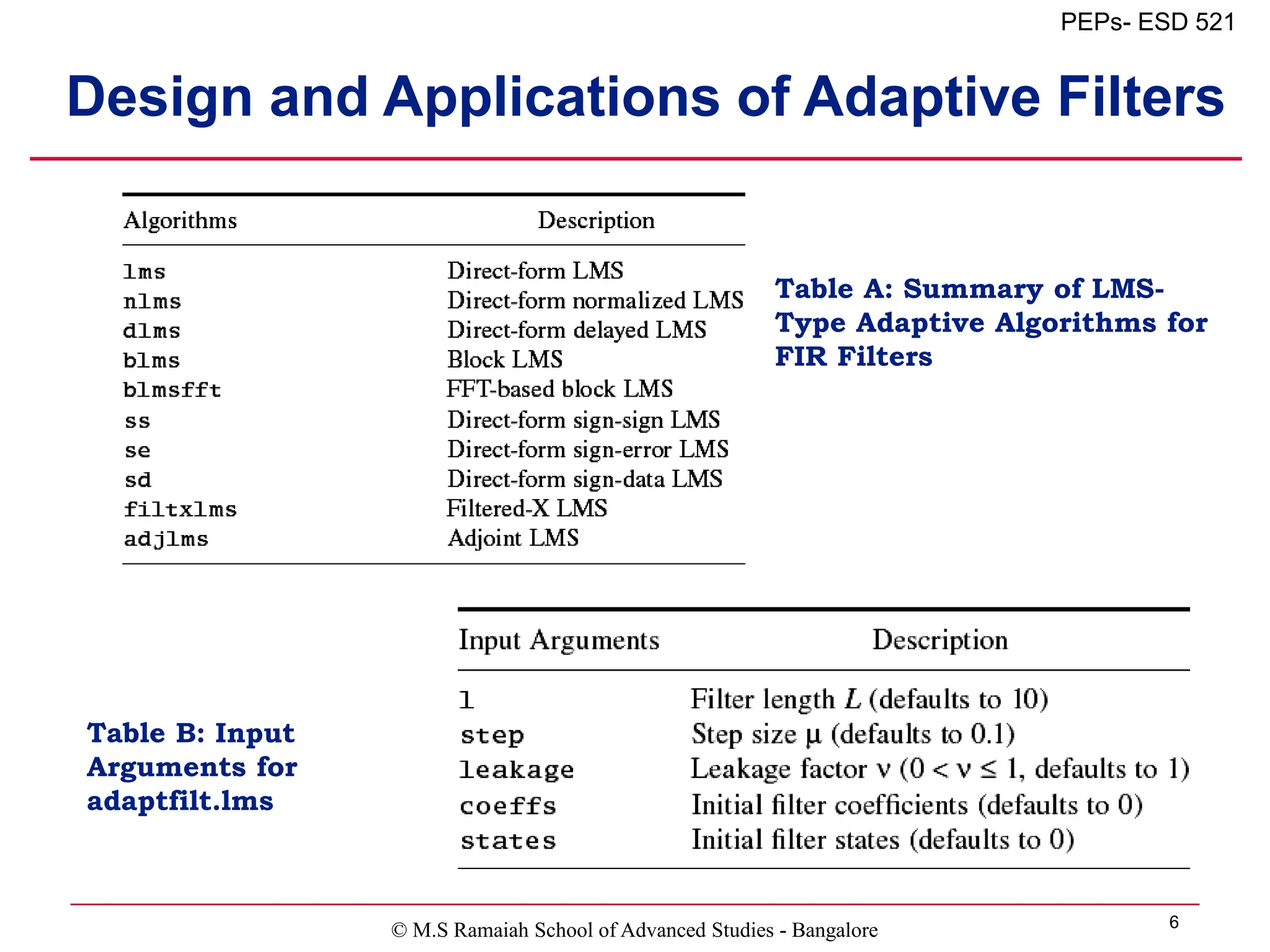
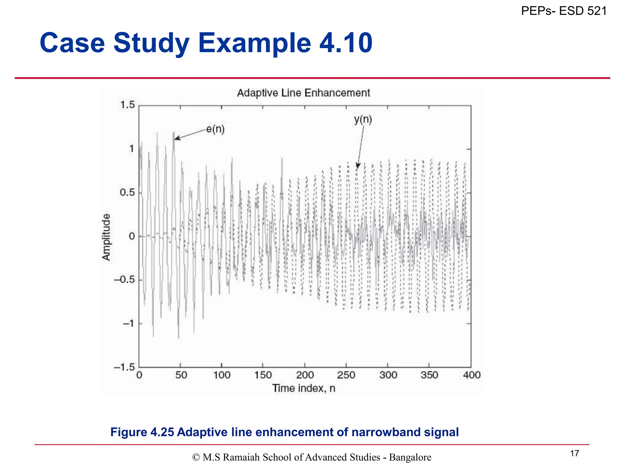
Case Study Example 4.10
Example 4.10
Description: (1) Mixing sinewave with white noise
(2) Use adaptive filter for enhancing sinewave
f = 400; fs = 4000; % signal parameters
N = 400; n = 0:1:N-1; % length and time index
sn = sin(2*pi*f*n/fs); % generate sinewave
noise=randn(size(sn)); % generate random noise
dn = sn+0.2*noise; % mixing sinewave with white noise
xn = dn; xn(1)=0; % generate x(n) using delay = 1
L = 64; % filter length
mu = 0.0005; % step size mu
ha = adaptfilt.lms(L,mu); % construct adaptive filter object
[y,e] = filter(ha,xn,dn); % adaptive filtering to get y(n) and e(n)
plot(n,y,':',n,e,'-');
title('Adaptive Line Enhancement');
xlabel('Time index, n'); ylabel('Amplitude');](https://image.slidesharecdn.com/adaptivefilters-231010073507-2e0fafed/75/Adaptive-Filters-ppt-16-2048.jpg)
![© M.S Ramaiah School of Advanced Studies - Bangalore 24
PEPs- ESD 521
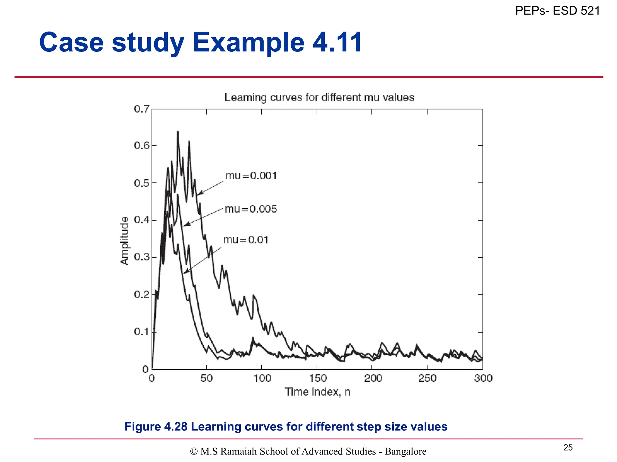
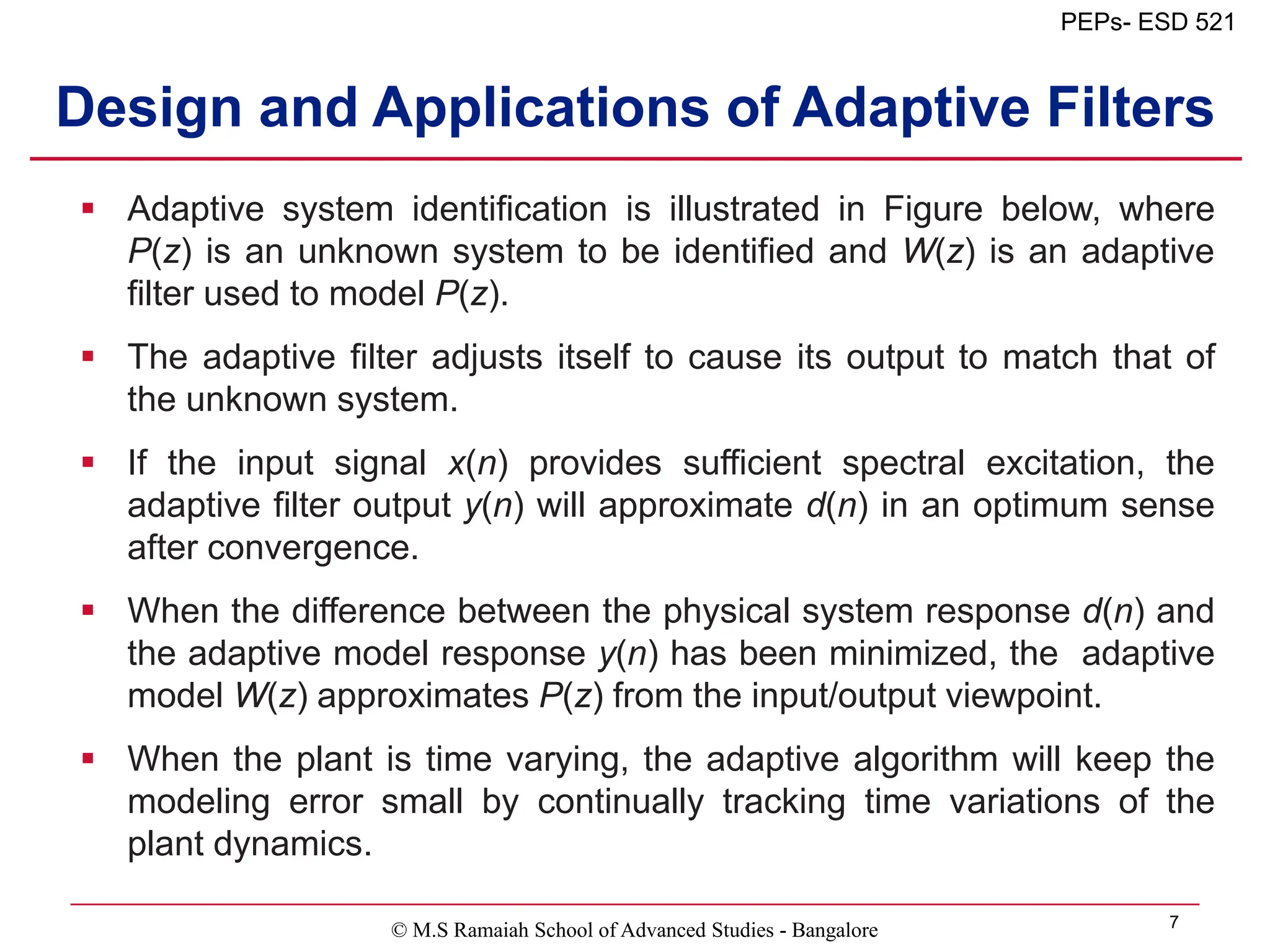
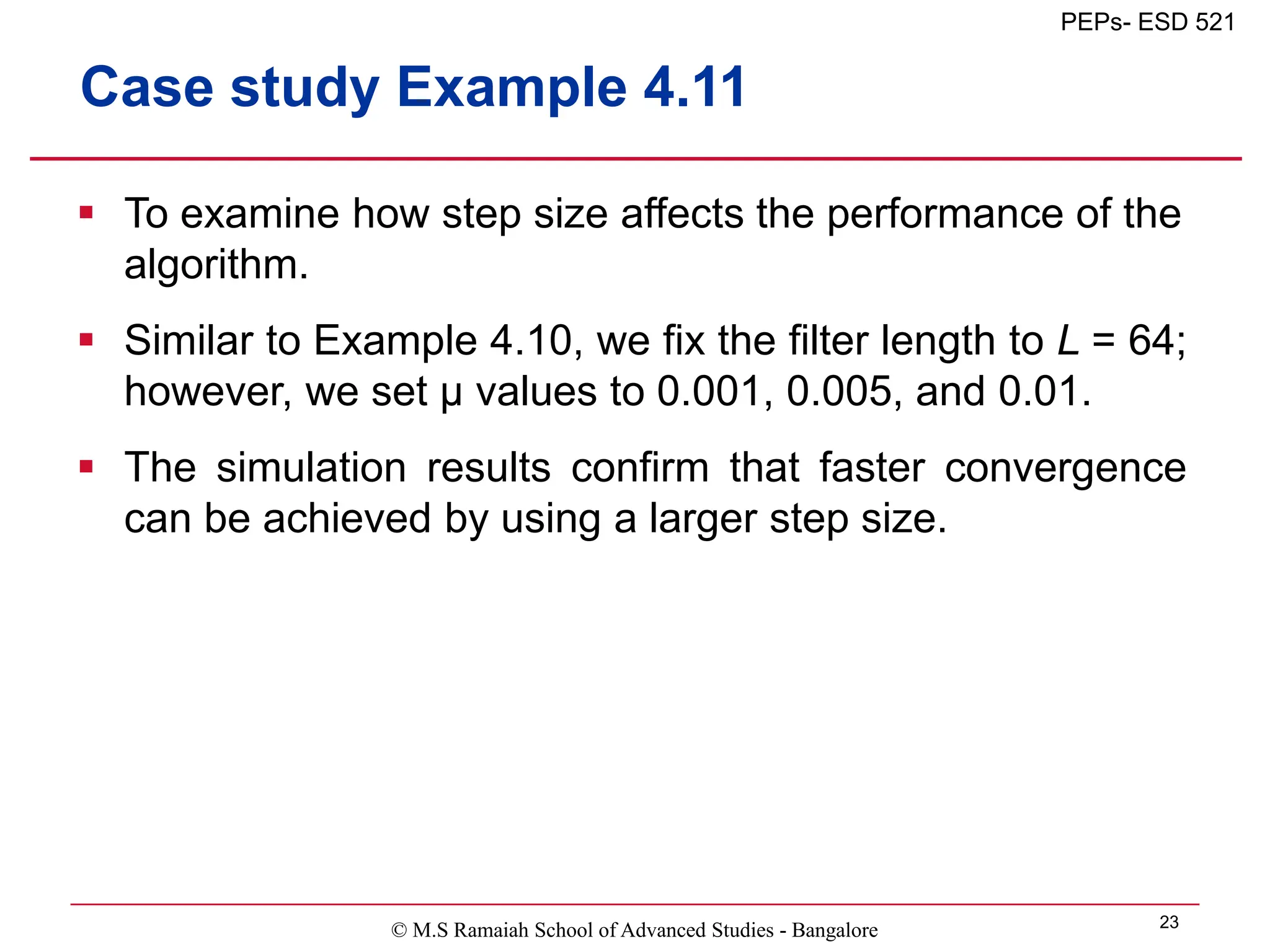
Example 4.11
Description: Examine how step size affects performance of
adaptive FIR filter with LMS algorithm
f = 400; fs = 4000; % signal parameters
N = 300; n = 0:1:N-1; % length and time index
sn = sin(2*pi*f*n/fs); % generate sinewave
noise=randn(size(sn)); % generate random noise
dn = sn+0.2*noise; % mixing sinewave with white noise
xn = dn; xn(1)=0; % generate x(n) using delay = 1
L = 64; % filter length
mu1 = 0.001; % step size mu1
mu2 = 0.005; % step size mu2
mu3 = 0.01; % step size mu3
ha1 = adaptfilt.lms(L,mu1); % construct adaptive filter object
[y1,e1] = filter(ha1,xn,dn);% adaptive filtering to get y(n) and e(n)
ha2 = adaptfilt.lms(L,mu2); % construct adaptive filter object
[y2,e2] = filter(ha2,xn,dn);% adaptive filtering to get y(n) and e(n)
ha3 = adaptfilt.lms(L,mu3); % construct adaptive filter object
[y3,e3] = filter(ha3,xn,dn);% adaptive filtering to get y(n) and e(n)
% learning curves
c1 = e1.*e1;
c2 = e2.*e2;
c3 = e3.*e3;
alpha = 0.1; b=alpha; a=[1 -(1-alpha)];
d1 = filter(b, a, c1);
d2 = filter(b, a, c2);
d3 = filter(b, a, c3);
plot(1:N,[d1;d2;d3]);
title('Learning curves for different mu values');
xlabel('Time index, n'); ylabel('Amplitude');](https://image.slidesharecdn.com/adaptivefilters-231010073507-2e0fafed/75/Adaptive-Filters-ppt-24-2048.jpg)