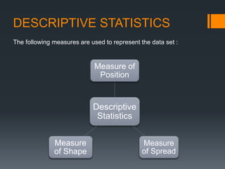
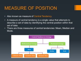
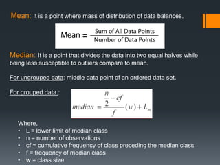
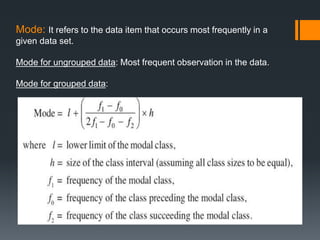
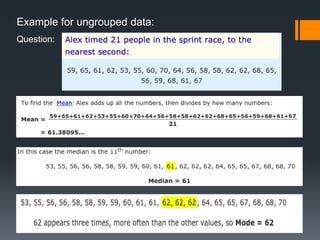
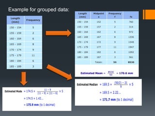
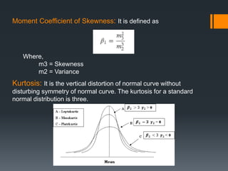
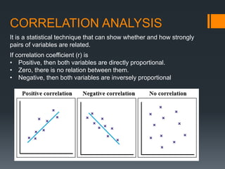
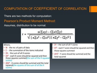
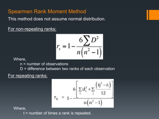
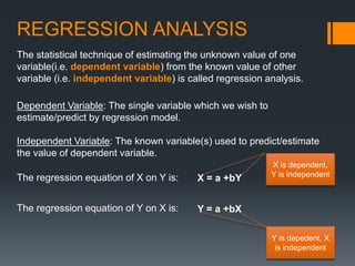
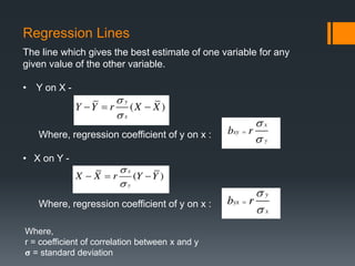
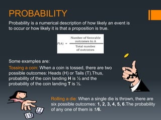
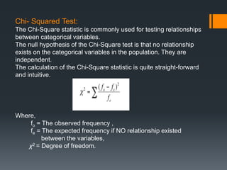
SlideShare a Scribd company logo
Introduction to Statistics and
Probability
STATISTICS
• It is the science of collecting, organizing, analyzing and interpreting
data.
• There are two types of Statistics:
Inferential Statistics : It is about using sample data from a dataset
and making inferences and conclusions using probability theory.
Descriptive Statistics: It is used to summarize and represent the
data in an accurate way using charts, tables and graphs.
For example, you might stand in a mall and ask a sample of 100
people if they like shopping at Sears. You could make a bar chart
of yes or no answers (that would be descriptive statistics) or you
could use your research (and inferential statistics) to reason that
around 75%-80% of population.
DESCRIPTIVE STATISTICS
The following measures are used to represent the data set :
Descriptive
Statistics
Measure of
Position
Measure
of Spread
Measure
of Shape
MEASURE OF POSITION
• Also known as measure of Central Tendency.
• A measure of central tendency is a single value that attempts to
describe a set of data by identifying the central position within that
set of data.
• There are three measures of central tendencies: Mean, Median and
Mode.
Median: It is a point that divides the data into two equal halves while
being less susceptible to outliers compare to mean.
For ungrouped data: middle data point of an ordered data set.
For grouped data :
Where,
• L = lower limit of median class
• n = number of observations
• cf = cumulative frequency of class preceding the median class
• f = frequency of median class
• w = class size
Mean: It is a point where mass of distribution of data balances.
Mode: It refers to the data item that occurs most frequently in a
given data set.
Mode for ungrouped data: Most frequent observation in the data.
Mode for grouped data:
Example for ungrouped data:
Question:
Example for grouped data:
MEASURE OF DISPERSION
• It refers to how the data deviates from the position measure i.e.
gives an indication of the amount of variation in the process.
• Dispersion of the data set can be described by:
Range: It is the difference between highest and the lowest values.
Standard Deviation: It is the measurement of average distance
between each quantity and mean i.e. how data is spread out from
mean. Higher the standard deviation, more is the data spread from
mean.
In normal distribution, when data is unimodal, z-scores is used to
calculate the probability of a score occurring within a standard
normal distribution and helps to compare two scores from different
samples.
Below, calculating the probability of randomly obtaining a score from
the distribution.
68% probability for -1 and +1 standard deviation from mean.
Similarly, 95% for -1.96 and +1.96 standard deviation.
MEASURE OF SHAPE
• It is used to characterize the location and variability of data set.
• Two common statistics that measure the shape of the data are:
Skewness and Kurtosis
Skewness : It is the horizontal displacement of the normal
curve about the mean position. Skewness for a normal distribution
is zero.
The methods to measure Skewness are:
Karl Pearson’s coefficient of Skewness: The value of coefficient
is between -1 and +1.
Bowley’s coefficient of Skewness: It is based on quartile value.
Where,
Q1 = First quartile
Q2 = Second quartile
Q3= Third quartile
Moment Coefficient of Skewness: It is defined as
Where,
m3 = Skewness
m2 = Variance
Kurtosis: It is the vertical distortion of normal curve without
disturbing symmetry of normal curve. The kurtosis for a standard
normal distribution is three.
CORRELATION ANALYSIS
It is a statistical technique that can show whether and how strongly
pairs of variables are related.
If correlation coefficient (r) is
• Positive, then both variables are directly proportional.
• Zero, there is no relation between them.
• Negative, then both variables are inversely proportional
Correlation: On the basis of number of variables
• Simple Correlation: It is when only two variables are analyzed.
For example, correlation between demand and supply.
• Partial Correlation: It is when two or more variables are
considered for analysis but only two influencing variables are
studied, rest are constant. For example, correlation between
demand, supply and income where income is constant.
• Multiple Correlation: It is when three or more variables are
analyzed simultaneously. For example, rainfall, production of rice
and price of rice are studied simultaneously.
COMPUTATION OF COEFFICIENT OF CORRELATION
There are two methods for computation:
Pearson’s Product Moment Method:
Assumes, distribution to be normal.
Spearmen Rank Moment Method
This method does not assume normal distribution.
For non-repeating ranks:
Where,
n = number of observations
D = difference between two ranks of each observation
For repeating ranks:
Where,
t = number of times a rank is repeated.
REGRESSION ANALYSIS
The statistical technique of estimating the unknown value of one
variable(i.e. dependent variable) from the known value of other
variable (i.e. independent variable) is called regression analysis.
The regression equation of X on Y is: X = a +bY
The regression equation of Y on X is: Y = a +bX
Dependent Variable: The single variable which we wish to
estimate/predict by regression model.
Independent Variable: The known variable(s) used to predict/estimate
the value of dependent variable.
X is dependent,
Y is independent
Y is depedent, X
is independent
Where, regression coefficient of y on x :
Where,
r = coefficient of correlation between x and y
𝛔 = standard deviation
Regression Lines
The line which gives the best estimate of one variable for any
given value of the other variable.
• Y on X -
• X on Y -
PROBABILITY
Probability is a numerical description of how likely an event is
to occur or how likely it is that a proposition is true.
Tossing a coin: When a coin is tossed, there are two
possible outcomes: Heads (H) or Tails (T).Thus,
probability of the coin landing H is ½ and the
probability of the coin landing T is ½.
Rolling a die: When a single die is thrown, there are
six possible outcomes: 1, 2, 3, 4, 5, 6.The probability
of any one of them is 1/6.
Some examples are:
TERMINOLOGY
Experiment: A process by which an outcome is obtained.
Sample space: The set S of all possible outcomes of an experiment.
i.e. the sample space for a dice roll is {1, 2, 3, 4, 5, 6}
Event: Any subset E of the sample space i.e.
Let,
E1 = An even number is rolled.
E2 = A number less than three is rolled.
Outcome: Result of a single trial.
Equally likely outcomes: Two outcomes of a random experiment
are said to be equally likely, if upon performing the experiment a (very)
large number of times, the relative occurrences of the two outcomes
turn out to be equal.
Trial: Performing a random experiment.
EVENTS
Simple Events : If the event E has only single element of a
sample space, it is called as a simple event. Eg: if S = {56 , 78 , 96 ,
54 , 89} and E = {78} then E is a simple event.
Compound Events: Any event consists of more than one
element of the sample space. Eg: if S = {56 ,78 ,96 ,54 ,89}, E1 =
{56 ,54 }, E2 = {78 ,56 ,89 } then, E1 and E2 represent two
compound events.
Independent Events and Dependent Events:
If the occurrence of any event is completely unaffected by the
occurrence of any other event, such events are Independent
Events.
Probability of two independent event is given by,
The events which are affected by other events are Dependent
Events.
Probability of dependent event is given by,
Exhaustive Events: A set of events is called exhaustive if all the
events together consume the entire sample space. Eg: A and B are
sets of mutually exclusive events,
Mutually Exclusive Events: If the occurrence of one event
excludes the occurrence of another event i.e. no two events can
occur simultaneously.
Where,
S = sample space
Addition Theorem
Theorem 1: If A and B are two mutually exclusive events, then
P(A ∪ B) = P(A) + P(B)
Where,
n = Total number of exhaustive cases
n1= Number of cases favorable to A.
n2= Number of cases favorable to B.
Theorem2: If A and B are two events that are not mutually exclusive,
then
P(A ∪ B) = P( A ) + P( B ) - P ( A ∩ B )
Where,
P (A ∩ B) = Probability of events favorable to both A and B
Multiplication Theorem
If A and B are two independent events, then the probability that both
will occur is equal to the product of their individual probabilities.
Example:
The probability of appointing a lecturer who is B.Com, MBA, and PhD,
with probabilities 1/20, 1/25 and 1/40 is given by:
Using multiplicative theorem for independent events,
Conditional Probability
The conditional probability of an event B is the probability that the event
will occur given the knowledge that an event A has already occurred. It
is representated as P( B | A).
P(A | B) = P(A ∩ B) ⁄ P(B)
Where A and B are two dependent events.
Total Probability Theorem
Given n mutually exclusive events A1, A2, … Ak such that their
probabilities sum is unity and their union is the event space E, then
Ai ∩ Aj = NULL, for all i not equal to j
A1 U A2 U ... U Ak = E
Then Total Probability Theorem or Law of Total Probability is:
where B is an arbitrary event, and P(B/Ai) is the conditional probability
of B assuming A already occurred.
Proof of Total Probability Theorem :
As intersection and Union are Distributive. Therefore,
B = (B ∩ A1) U (B ∩ A2) U ….... U (B ∩ AK)
Since all these partitions are disjoint. So, we have,
P (B ∩ A1) = P (B ∩ A1) U P(B ∩ A2) U ….... U P (B ∩ AK)
This is, addition theorem of probabilities for union of disjoint events.
Using Conditional Probability:
P (B / A) = P(B ∩ A) / P(A)
We know,
A1 U A2 U A3 U ….. U AK =
E(Total)Then, for any event B, we have,
B = B ∩ E
B = B ∩ (A1 U A2 U A3 U … U AK)
As the events are said to be independent here,
P(A ∩ B) = P(A) * P(B)
where P(B|A) is the conditional probability which gives the probability
of occurrence of event B when event A has already occurred. Hence,
P( B ∩ Ai ) = P( B | Ai ).P( Ai ) ; i = 1,2,3 . . . k
Applying this rule above:
This is Law of Total Probability.
It is used for evaluation of denominator in Bayes’ Theorem.
BAYES’ THEOREM
It is a mathematical formula for determining conditional probability.
In above formula, the posterior probability is equal to the conditional
probability of event B given A multiplied by the prior probability of A, all
divided by the prior probability of B.
Science itself is a special case of Bayes’
theorem because we are revising a prior
probability( hypothesis) in the light of
observation or experience that confirms our
hypothesis( experimental evidence) to develop
a posterior probability( conclusion)
Example Bayes’ Theorem:
Probability Distribution
BINOMIAL DISTRIBUTION
OF PROBABILITY
A binomial distribution is the probability of a SUCCESS or FAILURE
outcome in an experiment or survey that is repeated multiple times.
Criteria for binomial distribution:
• The number of observations or trials is fixed
• Each observation or trial is independent.
• The probability of success (tails, heads, fail or pass) is exactly the
same from one trial to another.
Example:
Q. A coin is tossed 10 times. What is the probability of getting exactly 6
heads?
The number of trials (n) is 10
x = 6
The odds of success (p) (tossing a heads) is 0.5
Odds of failure (q) = 1- p
P(x=6) = 10C6 * 0.5^6 * 0.5^4
= 210 * 0.015625 * 0.0625
= 0.205078125
POISSON DISTRIBUTION
OF PROBABILITY
The Poisson distribution is the discrete probability distribution of the
number of events occurring in a given time period, given the average
number of times the event occurs over that time period.
When the number of trials in a binomial distribution is very large, and
the probability of success is very small, then np ~ npq (as q ~ 1),
therefore it is possible to change the distribution to a Poisson
distribution.
Where,
x = 0,1,2,3….
ƛ = mean number of occurrences in the interval
e = Euler’s constant
Example:
Q. Twenty sheets of aluminum alloy were examined for surface flaws. The
frequency of the number of sheets with a given number of flaws per sheet was
as follows
The total number of flaws = (0x4)+(1x3)+(2x5)+(3x2+(4x4)+(5x1)+(6x1) = 46
So the average for 20 sheets (ℳ ) = 46/20 = 2.3
Probability = P(X>=3)
= 1 – (P(x0) +P(x1)+P(x2))
Using Poisson distribution formula
= 0.40396
What is the probability of finding a sheet chosen at random which contains 3
or more surface flaws?
Continuous Distribution
A probability distribution in which the
random variable X can take on any value
(is continuous) i.e. the probability of X
taking on any one specific value is zero.
Normal Distribution: A continuous random variable x is said to
follow normal distribution, if its probability density function is define
as follow,
Where, (μ)= means and (σ)= standard deviations.
Chi- Squared Test:
The Chi-Square statistic is commonly used for testing relationships
between categorical variables.
The null hypothesis of the Chi-Square test is that no relationship
exists on the categorical variables in the population. They are
independent.
The calculation of the Chi-Square statistic is quite straight-forward
and intuitive.
Where,
fo = The observed frequency ,
fe = The expected frequency if NO relationship existed
between the variables,
χ2 = Degree of freedom.
🤘

More Related Content

What's hot

PROBABILITY AND IT'S TYPES WITH RULES
PROBABILITY AND IT'S TYPES WITH RULESPROBABILITY AND IT'S TYPES WITH RULES
PROBABILITY AND IT'S TYPES WITH RULES
Bhargavi Bhanu
 
Discreet and continuous probability
Discreet and continuous probabilityDiscreet and continuous probability
Discreet and continuous probability
nj1992
 

What's hot (20)

Sample Space And Events
Sample Space And EventsSample Space And Events
Sample Space And Events
 
Basic Probability
Basic Probability Basic Probability
Basic Probability
 
Basic concepts of probability
Basic concepts of probabilityBasic concepts of probability
Basic concepts of probability
 
PROBABILITY AND IT'S TYPES WITH RULES
PROBABILITY AND IT'S TYPES WITH RULESPROBABILITY AND IT'S TYPES WITH RULES
PROBABILITY AND IT'S TYPES WITH RULES
 
Statistics: Probability
Statistics: ProbabilityStatistics: Probability
Statistics: Probability
 
Statistics & probability
Statistics & probabilityStatistics & probability
Statistics & probability
 
Probability
ProbabilityProbability
Probability
 
Probability
ProbabilityProbability
Probability
 
4.1-4.2 Sample Spaces and Probability
4.1-4.2 Sample Spaces and Probability4.1-4.2 Sample Spaces and Probability
4.1-4.2 Sample Spaces and Probability
 
Discrete and Continuous Random Variables
Discrete and Continuous Random VariablesDiscrete and Continuous Random Variables
Discrete and Continuous Random Variables
 
Introduction to Probability and Probability Distributions
Introduction to Probability and Probability DistributionsIntroduction to Probability and Probability Distributions
Introduction to Probability and Probability Distributions
 
Discreet and continuous probability
Discreet and continuous probabilityDiscreet and continuous probability
Discreet and continuous probability
 
Standard normal distribution
Standard normal distributionStandard normal distribution
Standard normal distribution
 
Probability (gr.11)
Probability (gr.11)Probability (gr.11)
Probability (gr.11)
 
Chapter 4 part2- Random Variables
Chapter 4 part2- Random VariablesChapter 4 part2- Random Variables
Chapter 4 part2- Random Variables
 
Basic probability concept
Basic probability conceptBasic probability concept
Basic probability concept
 
The Standard Normal Distribution
The Standard Normal Distribution  The Standard Normal Distribution
The Standard Normal Distribution
 
Point estimate for a population proportion p
Point estimate for a population proportion pPoint estimate for a population proportion p
Point estimate for a population proportion p
 
Random variable,Discrete and Continuous
Random variable,Discrete and ContinuousRandom variable,Discrete and Continuous
Random variable,Discrete and Continuous
 
Sample Space and Event,Probability,The Axioms of Probability,Bayes Theorem
Sample Space and Event,Probability,The Axioms of Probability,Bayes TheoremSample Space and Event,Probability,The Axioms of Probability,Bayes Theorem
Sample Space and Event,Probability,The Axioms of Probability,Bayes Theorem
 

Similar to Introduction to Statistics and Probability

CHAPTER 1 THEORY OF PROBABILITY AND STATISTICS.pptx
CHAPTER 1 THEORY OF PROBABILITY AND STATISTICS.pptxCHAPTER 1 THEORY OF PROBABILITY AND STATISTICS.pptx
CHAPTER 1 THEORY OF PROBABILITY AND STATISTICS.pptx
anshujain54751
 
Biostatistics
BiostatisticsBiostatistics
Biostatistics
priyarokz
 
MSC III_Research Methodology and Statistics_Inferrential ststistics.pdf
MSC III_Research Methodology and Statistics_Inferrential ststistics.pdfMSC III_Research Methodology and Statistics_Inferrential ststistics.pdf
MSC III_Research Methodology and Statistics_Inferrential ststistics.pdf
Suchita Rawat
 

Similar to Introduction to Statistics and Probability (20)

Descriptive Statistics
Descriptive StatisticsDescriptive Statistics
Descriptive Statistics
 
Basic Statistical Descriptions of Data.pptx
Basic Statistical Descriptions of Data.pptxBasic Statistical Descriptions of Data.pptx
Basic Statistical Descriptions of Data.pptx
 
Statistics and probability pp
Statistics and  probability ppStatistics and  probability pp
Statistics and probability pp
 
Inorganic CHEMISTRY
Inorganic CHEMISTRYInorganic CHEMISTRY
Inorganic CHEMISTRY
 
UNIT 4 PTRP final Convergence in probability.pptx
UNIT 4 PTRP final Convergence in probability.pptxUNIT 4 PTRP final Convergence in probability.pptx
UNIT 4 PTRP final Convergence in probability.pptx
 
Data science
Data scienceData science
Data science
 
Module-2_Notes-with-Example for data science
Module-2_Notes-with-Example for data scienceModule-2_Notes-with-Example for data science
Module-2_Notes-with-Example for data science
 
Types of Statistics
Types of Statistics Types of Statistics
Types of Statistics
 
CHAPTER 1 THEORY OF PROBABILITY AND STATISTICS.pptx
CHAPTER 1 THEORY OF PROBABILITY AND STATISTICS.pptxCHAPTER 1 THEORY OF PROBABILITY AND STATISTICS.pptx
CHAPTER 1 THEORY OF PROBABILITY AND STATISTICS.pptx
 
Statistics in research
Statistics in researchStatistics in research
Statistics in research
 
Biostatistics
BiostatisticsBiostatistics
Biostatistics
 
Descriptive Analysis.pptx
Descriptive Analysis.pptxDescriptive Analysis.pptx
Descriptive Analysis.pptx
 
Economic statistics ii -unit 2 & 5-(theory)
Economic statistics ii -unit 2 & 5-(theory)Economic statistics ii -unit 2 & 5-(theory)
Economic statistics ii -unit 2 & 5-(theory)
 
Statistics excellent
Statistics excellentStatistics excellent
Statistics excellent
 
MSC III_Research Methodology and Statistics_Inferrential ststistics.pdf
MSC III_Research Methodology and Statistics_Inferrential ststistics.pdfMSC III_Research Methodology and Statistics_Inferrential ststistics.pdf
MSC III_Research Methodology and Statistics_Inferrential ststistics.pdf
 
Overview of Advance Marketing Research
Overview of Advance Marketing ResearchOverview of Advance Marketing Research
Overview of Advance Marketing Research
 
Unit – III Spatial data Ajustment.pdf
Unit – III Spatial data Ajustment.pdfUnit – III Spatial data Ajustment.pdf
Unit – III Spatial data Ajustment.pdf
 
1.1 course notes inferential statistics
1.1 course notes inferential statistics1.1 course notes inferential statistics
1.1 course notes inferential statistics
 
The binomial distributions
The binomial distributionsThe binomial distributions
The binomial distributions
 
Factor Extraction method in factor analysis with example in R studio.pptx
Factor Extraction method in factor analysis with example in R studio.pptxFactor Extraction method in factor analysis with example in R studio.pptx
Factor Extraction method in factor analysis with example in R studio.pptx
 

Recently uploaded

Opendatabay - Open Data Marketplace.pptx
Opendatabay - Open Data Marketplace.pptxOpendatabay - Open Data Marketplace.pptx
Opendatabay - Open Data Marketplace.pptx
Opendatabay
 
一比一原版(YU毕业证)约克大学毕业证成绩单
一比一原版(YU毕业证)约克大学毕业证成绩单一比一原版(YU毕业证)约克大学毕业证成绩单
一比一原版(YU毕业证)约克大学毕业证成绩单
enxupq
 
Computer Presentation.pptx ecommerce advantage s
Computer Presentation.pptx ecommerce advantage sComputer Presentation.pptx ecommerce advantage s
Computer Presentation.pptx ecommerce advantage s
MAQIB18
 
Investigate & Recover / StarCompliance.io / Crypto_Crimes
Investigate & Recover / StarCompliance.io / Crypto_CrimesInvestigate & Recover / StarCompliance.io / Crypto_Crimes
Investigate & Recover / StarCompliance.io / Crypto_Crimes
StarCompliance.io
 
一比一原版(UPenn毕业证)宾夕法尼亚大学毕业证成绩单
一比一原版(UPenn毕业证)宾夕法尼亚大学毕业证成绩单一比一原版(UPenn毕业证)宾夕法尼亚大学毕业证成绩单
一比一原版(UPenn毕业证)宾夕法尼亚大学毕业证成绩单
ewymefz
 
一比一原版(IIT毕业证)伊利诺伊理工大学毕业证成绩单
一比一原版(IIT毕业证)伊利诺伊理工大学毕业证成绩单一比一原版(IIT毕业证)伊利诺伊理工大学毕业证成绩单
一比一原版(IIT毕业证)伊利诺伊理工大学毕业证成绩单
ewymefz
 
一比一原版(CU毕业证)卡尔顿大学毕业证成绩单
一比一原版(CU毕业证)卡尔顿大学毕业证成绩单一比一原版(CU毕业证)卡尔顿大学毕业证成绩单
一比一原版(CU毕业证)卡尔顿大学毕业证成绩单
yhkoc
 
Exploratory Data Analysis - Dilip S.pptx
Exploratory Data Analysis - Dilip S.pptxExploratory Data Analysis - Dilip S.pptx
Exploratory Data Analysis - Dilip S.pptx
DilipVasan
 

Recently uploaded (20)

Opendatabay - Open Data Marketplace.pptx
Opendatabay - Open Data Marketplace.pptxOpendatabay - Open Data Marketplace.pptx
Opendatabay - Open Data Marketplace.pptx
 
Innovative Methods in Media and Communication Research by Sebastian Kubitschk...
Innovative Methods in Media and Communication Research by Sebastian Kubitschk...Innovative Methods in Media and Communication Research by Sebastian Kubitschk...
Innovative Methods in Media and Communication Research by Sebastian Kubitschk...
 
Webinar One View, Multiple Systems No-Code Integration of Salesforce and ERPs
Webinar One View, Multiple Systems No-Code Integration of Salesforce and ERPsWebinar One View, Multiple Systems No-Code Integration of Salesforce and ERPs
Webinar One View, Multiple Systems No-Code Integration of Salesforce and ERPs
 
Slip-and-fall Injuries: Top Workers' Comp Claims
Slip-and-fall Injuries: Top Workers' Comp ClaimsSlip-and-fall Injuries: Top Workers' Comp Claims
Slip-and-fall Injuries: Top Workers' Comp Claims
 
一比一原版(YU毕业证)约克大学毕业证成绩单
一比一原版(YU毕业证)约克大学毕业证成绩单一比一原版(YU毕业证)约克大学毕业证成绩单
一比一原版(YU毕业证)约克大学毕业证成绩单
 
Supply chain analytics to combat the effects of Ukraine-Russia-conflict
Supply chain analytics to combat the effects of Ukraine-Russia-conflictSupply chain analytics to combat the effects of Ukraine-Russia-conflict
Supply chain analytics to combat the effects of Ukraine-Russia-conflict
 
Computer Presentation.pptx ecommerce advantage s
Computer Presentation.pptx ecommerce advantage sComputer Presentation.pptx ecommerce advantage s
Computer Presentation.pptx ecommerce advantage s
 
Investigate & Recover / StarCompliance.io / Crypto_Crimes
Investigate & Recover / StarCompliance.io / Crypto_CrimesInvestigate & Recover / StarCompliance.io / Crypto_Crimes
Investigate & Recover / StarCompliance.io / Crypto_Crimes
 
一比一原版(UPenn毕业证)宾夕法尼亚大学毕业证成绩单
一比一原版(UPenn毕业证)宾夕法尼亚大学毕业证成绩单一比一原版(UPenn毕业证)宾夕法尼亚大学毕业证成绩单
一比一原版(UPenn毕业证)宾夕法尼亚大学毕业证成绩单
 
Jpolillo Amazon PPC - Bid Optimization Sample
Jpolillo Amazon PPC - Bid Optimization SampleJpolillo Amazon PPC - Bid Optimization Sample
Jpolillo Amazon PPC - Bid Optimization Sample
 
Pre-ProductionImproveddsfjgndflghtgg.pptx
Pre-ProductionImproveddsfjgndflghtgg.pptxPre-ProductionImproveddsfjgndflghtgg.pptx
Pre-ProductionImproveddsfjgndflghtgg.pptx
 
一比一原版(IIT毕业证)伊利诺伊理工大学毕业证成绩单
一比一原版(IIT毕业证)伊利诺伊理工大学毕业证成绩单一比一原版(IIT毕业证)伊利诺伊理工大学毕业证成绩单
一比一原版(IIT毕业证)伊利诺伊理工大学毕业证成绩单
 
一比一原版(CU毕业证)卡尔顿大学毕业证成绩单
一比一原版(CU毕业证)卡尔顿大学毕业证成绩单一比一原版(CU毕业证)卡尔顿大学毕业证成绩单
一比一原版(CU毕业证)卡尔顿大学毕业证成绩单
 
How can I successfully sell my pi coins in Philippines?
How can I successfully sell my pi coins in Philippines?How can I successfully sell my pi coins in Philippines?
How can I successfully sell my pi coins in Philippines?
 
Q1’2024 Update: MYCI’s Leap Year Rebound
Q1’2024 Update: MYCI’s Leap Year ReboundQ1’2024 Update: MYCI’s Leap Year Rebound
Q1’2024 Update: MYCI’s Leap Year Rebound
 
Using PDB Relocation to Move a Single PDB to Another Existing CDB
Using PDB Relocation to Move a Single PDB to Another Existing CDBUsing PDB Relocation to Move a Single PDB to Another Existing CDB
Using PDB Relocation to Move a Single PDB to Another Existing CDB
 
Exploratory Data Analysis - Dilip S.pptx
Exploratory Data Analysis - Dilip S.pptxExploratory Data Analysis - Dilip S.pptx
Exploratory Data Analysis - Dilip S.pptx
 
Business update Q1 2024 Lar España Real Estate SOCIMI
Business update Q1 2024 Lar España Real Estate SOCIMIBusiness update Q1 2024 Lar España Real Estate SOCIMI
Business update Q1 2024 Lar España Real Estate SOCIMI
 
社内勉強会資料_LLM Agents                              .
社内勉強会資料_LLM Agents                              .社内勉強会資料_LLM Agents                              .
社内勉強会資料_LLM Agents                              .
 
Tabula.io Cheatsheet: automate your data workflows
Tabula.io Cheatsheet: automate your data workflowsTabula.io Cheatsheet: automate your data workflows
Tabula.io Cheatsheet: automate your data workflows
 

Introduction to Statistics and Probability

  • 1. Introduction to Statistics and Probability
  • 2. STATISTICS • It is the science of collecting, organizing, analyzing and interpreting data. • There are two types of Statistics: Inferential Statistics : It is about using sample data from a dataset and making inferences and conclusions using probability theory. Descriptive Statistics: It is used to summarize and represent the data in an accurate way using charts, tables and graphs. For example, you might stand in a mall and ask a sample of 100 people if they like shopping at Sears. You could make a bar chart of yes or no answers (that would be descriptive statistics) or you could use your research (and inferential statistics) to reason that around 75%-80% of population.
  • 3. DESCRIPTIVE STATISTICS The following measures are used to represent the data set : Descriptive Statistics Measure of Position Measure of Spread Measure of Shape
  • 4. MEASURE OF POSITION • Also known as measure of Central Tendency. • A measure of central tendency is a single value that attempts to describe a set of data by identifying the central position within that set of data. • There are three measures of central tendencies: Mean, Median and Mode.
  • 5. Median: It is a point that divides the data into two equal halves while being less susceptible to outliers compare to mean. For ungrouped data: middle data point of an ordered data set. For grouped data : Where, • L = lower limit of median class • n = number of observations • cf = cumulative frequency of class preceding the median class • f = frequency of median class • w = class size Mean: It is a point where mass of distribution of data balances.
  • 6. Mode: It refers to the data item that occurs most frequently in a given data set. Mode for ungrouped data: Most frequent observation in the data. Mode for grouped data:
  • 7. Example for ungrouped data: Question:
  • 9. MEASURE OF DISPERSION • It refers to how the data deviates from the position measure i.e. gives an indication of the amount of variation in the process. • Dispersion of the data set can be described by: Range: It is the difference between highest and the lowest values. Standard Deviation: It is the measurement of average distance between each quantity and mean i.e. how data is spread out from mean. Higher the standard deviation, more is the data spread from mean.
  • 10. In normal distribution, when data is unimodal, z-scores is used to calculate the probability of a score occurring within a standard normal distribution and helps to compare two scores from different samples. Below, calculating the probability of randomly obtaining a score from the distribution. 68% probability for -1 and +1 standard deviation from mean. Similarly, 95% for -1.96 and +1.96 standard deviation.
  • 11. MEASURE OF SHAPE • It is used to characterize the location and variability of data set. • Two common statistics that measure the shape of the data are: Skewness and Kurtosis Skewness : It is the horizontal displacement of the normal curve about the mean position. Skewness for a normal distribution is zero.
  • 12. The methods to measure Skewness are: Karl Pearson’s coefficient of Skewness: The value of coefficient is between -1 and +1. Bowley’s coefficient of Skewness: It is based on quartile value. Where, Q1 = First quartile Q2 = Second quartile Q3= Third quartile
  • 13. Moment Coefficient of Skewness: It is defined as Where, m3 = Skewness m2 = Variance Kurtosis: It is the vertical distortion of normal curve without disturbing symmetry of normal curve. The kurtosis for a standard normal distribution is three.
  • 14. CORRELATION ANALYSIS It is a statistical technique that can show whether and how strongly pairs of variables are related. If correlation coefficient (r) is • Positive, then both variables are directly proportional. • Zero, there is no relation between them. • Negative, then both variables are inversely proportional
  • 15. Correlation: On the basis of number of variables • Simple Correlation: It is when only two variables are analyzed. For example, correlation between demand and supply. • Partial Correlation: It is when two or more variables are considered for analysis but only two influencing variables are studied, rest are constant. For example, correlation between demand, supply and income where income is constant. • Multiple Correlation: It is when three or more variables are analyzed simultaneously. For example, rainfall, production of rice and price of rice are studied simultaneously.
  • 16. COMPUTATION OF COEFFICIENT OF CORRELATION There are two methods for computation: Pearson’s Product Moment Method: Assumes, distribution to be normal.
  • 17. Spearmen Rank Moment Method This method does not assume normal distribution. For non-repeating ranks: Where, n = number of observations D = difference between two ranks of each observation For repeating ranks: Where, t = number of times a rank is repeated.
  • 18. REGRESSION ANALYSIS The statistical technique of estimating the unknown value of one variable(i.e. dependent variable) from the known value of other variable (i.e. independent variable) is called regression analysis. The regression equation of X on Y is: X = a +bY The regression equation of Y on X is: Y = a +bX Dependent Variable: The single variable which we wish to estimate/predict by regression model. Independent Variable: The known variable(s) used to predict/estimate the value of dependent variable. X is dependent, Y is independent Y is depedent, X is independent
  • 19. Where, regression coefficient of y on x : Where, regression coefficient of y on x : Where, r = coefficient of correlation between x and y 𝛔 = standard deviation Regression Lines The line which gives the best estimate of one variable for any given value of the other variable. • Y on X - • X on Y -
  • 20. PROBABILITY Probability is a numerical description of how likely an event is to occur or how likely it is that a proposition is true. Tossing a coin: When a coin is tossed, there are two possible outcomes: Heads (H) or Tails (T).Thus, probability of the coin landing H is ½ and the probability of the coin landing T is ½. Rolling a die: When a single die is thrown, there are six possible outcomes: 1, 2, 3, 4, 5, 6.The probability of any one of them is 1/6. Some examples are:
  • 21. TERMINOLOGY Experiment: A process by which an outcome is obtained. Sample space: The set S of all possible outcomes of an experiment. i.e. the sample space for a dice roll is {1, 2, 3, 4, 5, 6} Event: Any subset E of the sample space i.e. Let, E1 = An even number is rolled. E2 = A number less than three is rolled. Outcome: Result of a single trial. Equally likely outcomes: Two outcomes of a random experiment are said to be equally likely, if upon performing the experiment a (very) large number of times, the relative occurrences of the two outcomes turn out to be equal. Trial: Performing a random experiment.
  • 22. EVENTS Simple Events : If the event E has only single element of a sample space, it is called as a simple event. Eg: if S = {56 , 78 , 96 , 54 , 89} and E = {78} then E is a simple event. Compound Events: Any event consists of more than one element of the sample space. Eg: if S = {56 ,78 ,96 ,54 ,89}, E1 = {56 ,54 }, E2 = {78 ,56 ,89 } then, E1 and E2 represent two compound events. Independent Events and Dependent Events: If the occurrence of any event is completely unaffected by the occurrence of any other event, such events are Independent Events. Probability of two independent event is given by,
  • 23. The events which are affected by other events are Dependent Events. Probability of dependent event is given by, Exhaustive Events: A set of events is called exhaustive if all the events together consume the entire sample space. Eg: A and B are sets of mutually exclusive events, Mutually Exclusive Events: If the occurrence of one event excludes the occurrence of another event i.e. no two events can occur simultaneously. Where, S = sample space
  • 24. Addition Theorem Theorem 1: If A and B are two mutually exclusive events, then P(A ∪ B) = P(A) + P(B) Where, n = Total number of exhaustive cases n1= Number of cases favorable to A. n2= Number of cases favorable to B. Theorem2: If A and B are two events that are not mutually exclusive, then P(A ∪ B) = P( A ) + P( B ) - P ( A ∩ B ) Where, P (A ∩ B) = Probability of events favorable to both A and B
  • 25. Multiplication Theorem If A and B are two independent events, then the probability that both will occur is equal to the product of their individual probabilities. Example: The probability of appointing a lecturer who is B.Com, MBA, and PhD, with probabilities 1/20, 1/25 and 1/40 is given by: Using multiplicative theorem for independent events,
  • 26. Conditional Probability The conditional probability of an event B is the probability that the event will occur given the knowledge that an event A has already occurred. It is representated as P( B | A). P(A | B) = P(A ∩ B) ⁄ P(B) Where A and B are two dependent events.
  • 27. Total Probability Theorem Given n mutually exclusive events A1, A2, … Ak such that their probabilities sum is unity and their union is the event space E, then Ai ∩ Aj = NULL, for all i not equal to j A1 U A2 U ... U Ak = E Then Total Probability Theorem or Law of Total Probability is: where B is an arbitrary event, and P(B/Ai) is the conditional probability of B assuming A already occurred.
  • 28. Proof of Total Probability Theorem : As intersection and Union are Distributive. Therefore, B = (B ∩ A1) U (B ∩ A2) U ….... U (B ∩ AK) Since all these partitions are disjoint. So, we have, P (B ∩ A1) = P (B ∩ A1) U P(B ∩ A2) U ….... U P (B ∩ AK) This is, addition theorem of probabilities for union of disjoint events. Using Conditional Probability: P (B / A) = P(B ∩ A) / P(A) We know, A1 U A2 U A3 U ….. U AK = E(Total)Then, for any event B, we have, B = B ∩ E B = B ∩ (A1 U A2 U A3 U … U AK)
  • 29. As the events are said to be independent here, P(A ∩ B) = P(A) * P(B) where P(B|A) is the conditional probability which gives the probability of occurrence of event B when event A has already occurred. Hence, P( B ∩ Ai ) = P( B | Ai ).P( Ai ) ; i = 1,2,3 . . . k Applying this rule above: This is Law of Total Probability. It is used for evaluation of denominator in Bayes’ Theorem.
  • 30. BAYES’ THEOREM It is a mathematical formula for determining conditional probability. In above formula, the posterior probability is equal to the conditional probability of event B given A multiplied by the prior probability of A, all divided by the prior probability of B. Science itself is a special case of Bayes’ theorem because we are revising a prior probability( hypothesis) in the light of observation or experience that confirms our hypothesis( experimental evidence) to develop a posterior probability( conclusion)
  • 33. BINOMIAL DISTRIBUTION OF PROBABILITY A binomial distribution is the probability of a SUCCESS or FAILURE outcome in an experiment or survey that is repeated multiple times. Criteria for binomial distribution: • The number of observations or trials is fixed • Each observation or trial is independent. • The probability of success (tails, heads, fail or pass) is exactly the same from one trial to another.
  • 34. Example: Q. A coin is tossed 10 times. What is the probability of getting exactly 6 heads? The number of trials (n) is 10 x = 6 The odds of success (p) (tossing a heads) is 0.5 Odds of failure (q) = 1- p P(x=6) = 10C6 * 0.5^6 * 0.5^4 = 210 * 0.015625 * 0.0625 = 0.205078125
  • 35. POISSON DISTRIBUTION OF PROBABILITY The Poisson distribution is the discrete probability distribution of the number of events occurring in a given time period, given the average number of times the event occurs over that time period. When the number of trials in a binomial distribution is very large, and the probability of success is very small, then np ~ npq (as q ~ 1), therefore it is possible to change the distribution to a Poisson distribution. Where, x = 0,1,2,3…. ƛ = mean number of occurrences in the interval e = Euler’s constant
  • 36. Example: Q. Twenty sheets of aluminum alloy were examined for surface flaws. The frequency of the number of sheets with a given number of flaws per sheet was as follows The total number of flaws = (0x4)+(1x3)+(2x5)+(3x2+(4x4)+(5x1)+(6x1) = 46 So the average for 20 sheets (ℳ ) = 46/20 = 2.3 Probability = P(X>=3) = 1 – (P(x0) +P(x1)+P(x2)) Using Poisson distribution formula = 0.40396 What is the probability of finding a sheet chosen at random which contains 3 or more surface flaws?
  • 37. Continuous Distribution A probability distribution in which the random variable X can take on any value (is continuous) i.e. the probability of X taking on any one specific value is zero. Normal Distribution: A continuous random variable x is said to follow normal distribution, if its probability density function is define as follow, Where, (μ)= means and (σ)= standard deviations.
  • 38. Chi- Squared Test: The Chi-Square statistic is commonly used for testing relationships between categorical variables. The null hypothesis of the Chi-Square test is that no relationship exists on the categorical variables in the population. They are independent. The calculation of the Chi-Square statistic is quite straight-forward and intuitive. Where, fo = The observed frequency , fe = The expected frequency if NO relationship existed between the variables, χ2 = Degree of freedom.
  • 39. 🤘