PPT, PDF224 views

Digital Elevation Model - DEM, DSM, DTM

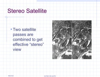
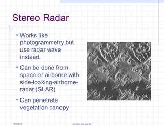
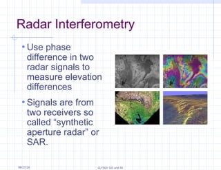
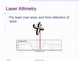
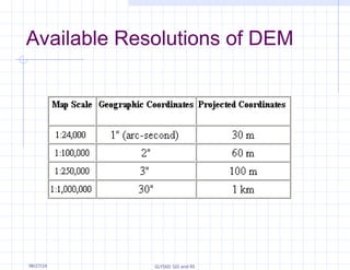
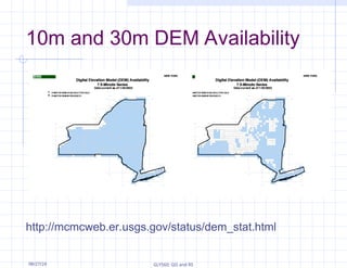
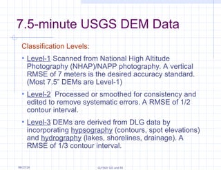
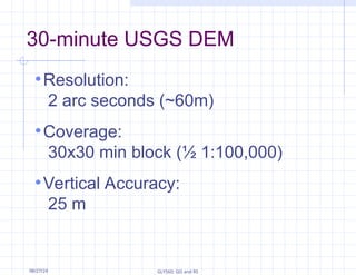
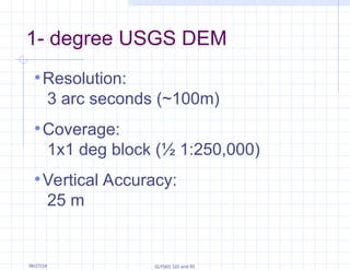
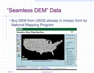
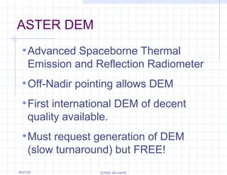
The document outlines various methods for creating digital elevation models (DEMs) used in GIS and remote sensing, including photogrammetry, satellite stereo, radar stereo, radar interferometry, and laser altimetry. It details the resolution, coverage, and vertical accuracy of different USGS DEM classifications and global DEMs like GTOPO30 and ASTER. Additionally, it provides information on data availability and processing standards for DEMs.

Education◦

1 / 19

2 / 19

3 / 19

Digital Elevation Model - DEM, DSM, DTM

1.
Digital Elevation Models GLY560: GIS and Remote Sensing for Earth Scientists Class Home Page: http://www.geology.buffalo.edu/courses/gly560/
2.
08/27/24 GLY560: GISand RS Creation of DEM’s •Conversion of contour lines •Photogrammetry •Satellite Stereo •Radar Stereo •Radar Inferometry •Laser Altimetry
3.
08/27/24 GLY560: GISand RS Conversion of printed contour lines • Existing map plates are scanned • Resulting raster is vectorized and edited contours are "tagged" with elevations • Additional elevation data are created from the hydrography layer (e.g. shorelines provide additional contours) • Algorithm is used to interpolate elevations at every grid point from the contour data
4.
08/27/24 GLY560: GISand RS Photogrammetry • Manually: an operator looks at a pair of stereophotos through a stereoplotter and must move two dots together until they appear to be one lying just at the surface of the ground • Automatically: an instrument calculates the parallax displacement of a large number of points (e.g. for USGS 7.5 minute quadrangles, the Gestalt Photo Mapper II correlates 500,000 points) • Correction of elevation from photographs: water bodies are assumed to be flat.
5.
08/27/24 GLY560: GISand RS Stereo Satellite • Two satellite passes are combined to get effective “stereo” view
6.
08/27/24 GLY560: GISand RS Stereo Radar • Works like photogrammetry but use radar wave instead. • Can be done from space or airborne with side-looking-airborne- radar (SLAR) • Can penetrate vegetation canopy
7.
08/27/24 GLY560: GISand RS Radar Interferometry • Use phase difference in two radar signals to measure elevation differences • Signals are from two receivers so called “synthetic aperture radar” or SAR.
8.
08/27/24 GLY560: GISand RS Laser Altimetry • Fly laser over area, and time reflection of laser.
9.
08/27/24 GLY560: GISand RS Available Resolutions of DEM
10.
08/27/24 GLY560: GISand RS 7.5-minute USGS DEM •Resolution: 10 m or 30 m •Coverage: 7.5 x 7.5 min Quad (1:24,000) •Vertical Accuracy: 7 m
11.
08/27/24 GLY560: GISand RS 10m and 30m DEM Availability http://mcmcweb.er.usgs.gov/status/dem_stat.html
12.
08/27/24 GLY560: GISand RS 7.5-minute USGS DEM Data Classification Levels: • Level-1 Scanned from National High Altitude Photography (NHAP)/NAPP photography. A vertical RMSE of 7 meters is the desired accuracy standard. (Most 7.5” DEMs are Level-1) • Level-2 Processed or smoothed for consistency and edited to remove systematic errors. A RMSE of 1/2 contour interval. • Level-3 DEMs are derived from DLG data by incorporating hypsography (contours, spot elevations) and hydrography (lakes, shorelines, drainage). A RMSE of 1/3 contour interval.
13.
08/27/24 GLY560: GISand RS 30-minute USGS DEM •Resolution: 2 arc seconds (~60m) •Coverage: 30x30 min block (½ 1:100,000) •Vertical Accuracy: 25 m
14.
08/27/24 GLY560: GISand RS 1- degree USGS DEM •Resolution: 3 arc seconds (~100m) •Coverage: 1x1 deg block (½ 1:250,000) •Vertical Accuracy: 25 m
15.
08/27/24 GLY560: GISand RS “Seamless DEM” Data • Buy DEM from USGS already in mosaic form by National Mapping Program
16.
08/27/24 GLY560: GISand RS Global DEMs •GTOPO30 •Aster •Shuttle Mapping Program •IKONOS
17.
08/27/24 GLY560: GISand RS GTOPO30 •Resolution: 30-second (~1 km) •Coverage: 50 deg lat x 40 deg long •Vertical Accuracy: 30 m
18.
08/27/24 GLY560: GISand RS ASTER DEM •Advanced Spaceborne Thermal Emission and Reflection Radiometer •Off-Nadir pointing allows DEM •First international DEM of decent quality available. •Must request generation of DEM (slow turnaround) but FREE!
19.
08/27/24 GLY560: GISand RS Aster DEM • GTOPO30 (1 km2 /pixel) • ASTER (30 m2 /pixel)

Editor's Notes

#7 Synthetic Aperture Radar images, generated simultaneously from two antennas on the same platform, have such a small base that they do not, in themselves, function as a stereo pair. But being composed of coherent radiation, signals from each, matched to equivalent pixels in the other, show varying degrees of phase differences, indicative of partial interference. Variations in the signal travel times between two adjacent points induce the interference, and thus, show slightly different heights. When we remove Earth curvature effects and make other adjustments, residual differences become a measure of terrain elevations.
#18 Digital Terrain Modeling and Mapping Terrain Modeling and Mapping using DEM, SDTS, DRG, DLG DTED and ASTER Data jchilds@terrainmap.com ASTER DEM! Until just recently, I knew of only two sources of free international DEM data. The first is the 1 km DTED0 data available from NIMA (and the equivalent GTOPO30 data set available from USGS/EOS). The second was the reverse engineering approach of extracting DEMs from topo maps as described in my earlier article. Of course IKONOS and QuickBird commercial satellite imagery are (or will soon be, in the case of QuickBird) available, but although of excellent quality, this data is quite expensive. (The Digital Globe website quotes prices of $25/square kilometer. This equates to about $3,500 for a 1:24000 USGS quad.) However, there is another source of international DEM data that has been known to the scientific community and few others until recently: ASTER (Advanced Spaceborne Thermal Emission and Reflection Radiometer). The quality of this data is excellent, equivalent in resolution to USGS 30m SDTS DEM data. ASTER is an imaging instrument that is flying on the TERRA satellite launched in December 1999 as part of NASA's Earth Observing System (EOS). ASTER represents a revolution in the remote sensing community because of the availability of its imagery and its superior resolution. ASTER resolution ranges from 15m to 90m, depending on the wavelength. The instrument records in three bands: the Visible and Near Infrared (VNIR ), the Shortwave Infrared (SWIR ), and the Thermal Infrared (TIR ), oriented on the nadir and backward looking. There are 14 spectral bands all together spanning the visible and infrared spectra, so the sensor is susceptible to cloud cover and cannot record images at night. Because of its off-nadir sensor pointing capability, ASTER can collect the stereo pairs necessary to generate high resolution DEMS (using bands 3N and 3B). Instead of the woeful 1km resolution DTED0 data, ASTER DEMs offer a very respectable 30m resolution. The EOS ground stations archive imagery corresponding to the spectral bands of the ASTER sensors, including the Level 1A data sets. The DEMs are assembled from this data. Once produced, EOS archives the DEMs in its database so that they will be available essentially immediately upon subsequent request. If the DEM you are interested in is not in the archive, all is not lost. You can enter your request for DEM production into a queue. Your DEM will be constructed by EOS from the L1A data. This can take anywhere from two to ten weeks. Another option is to construct the DEMs yourself using the appropriate software. (It is also reportedly possible to order a fly-by acquisition, but this method is not publicized by NASA and is probably by special arrangement for government and academic researchers.) Why does ASTER represent a revolution in the world of terrain modeling? Because its 30m resolution is the same as the classified NIMA DTED1 data set. NIMA has never released its DTED1 series of DEM data and in fact is doing its best to block NASA from releasing 30m SRTM data from the Space Shuttle. (Quote from the NASA SRTM website:"Following the events of Sept. 11, 2001 our project partners in the National Imagery and Mapping Agency have requested that NASA and JPL not distribute any SRTM data to the scientific community or the public, including shaded relief maps or other visualizations. We look forward to this restriction being lifted soon so data may be made publicly available." NIMA does not feel it is necessary to explain what the events of September 11 have to do with DEMs of someplace like Mt. Aconcagua in Argentina, for example, or how long "soon" might be.) However, NASA somehow overcame whatever reservations NIMA might have had concerning ASTER. This is (pleasantly) surprising considering NIMA's position on the SRTM situation. It is hard to believe that NIMA does not know about the EOS Data Gateway, despite its obscurity. On the other hand, how does NIMA rationalize its position on the SRTM data in light of the unrestricted availability of ASTER data of similar quality? I believe it is time for the ASTER client base to expand from its current concentration in the academic and governmental community to the broader public GIS sector. In this way the continued availability of this valuable data source may be assured by the strength of our larger numbers. What does ASTER resolution mean to the terrain modeler? Consider the first image at top right. It is an ASTER DEM of the Jordan river valley in the occupied West Bank of Israel. The image is approximately 2500 by 2500 postings large, covering an area of about 75 square kilometers. The image immediately below is a section of NIMA DTED0 quad N32E035, covering approximately the same area. Because of the inferior resolution of the DTED0 image, it is hard to believe that the coverages coincide very closely. Before ASTER, this was effectively the highest resolution DEM available to the civilian public. This DEM contains 232 by 246 individual elevation postings. The point should be obvious. The ASTER image contains more than 100 times as much data as the DTED0 image. Despite only being in orbit since February, 2000, ASTER has already accumulated a relatively large archive of imagery. This data is offered for essentially free download from the EOS Data Gateway. However, the procedure for downloading the data is not particularly easy. You have to navigate a somewhat awkward and slow user interface. After placing your order using a four-step process, you must wait anywhere from one hour to two days for your image to become available for archived images, and as long as ten weeks if you request production of a DEM not in the archive. You download the data from a designated anonymous ftp site using an ftp utility like WS_FTP or the DOS command line. Another obstacle is the file format. ASTER imagery is offered in something called HDF-EOS. HDF is yet another cumbersome, complicated self-describing scientific file format that few applications recognize. Those that do are all generalized HDF readers that are necessarily complex because they must accommodate all types of scientific data sets that may be packaged in HDF format. (In general, HDF data may not even be image data.) The DEM files are also offered in a 16-bit GeoTiff format. This does not represent much of an advantage, because most graphics applications only read the more common 24-bit tiff format. Even if they could read it, very few applications know what to do with a GeoTiff DEM once they get it, since the format was really designed to accommodate 2D spatial data. (One that does due to recent upgrades is GlobalMapper). ASTER DEMs are also quite large. Each file is about 12 MB in either of the two formats. This makes converting and transporting the files from one application to another a challenge. Of course I wrote yet another converter, this one called GEOTIFF to help with this problem. This program takes ASTER Geotiff DEMs and converts them to USGS native DEM format. (SDTS would have been a better choice for output because of its binary format, but the SDTS format is very complicated to write, and I already had a USGS DEM writer. So this was the expedient choice.) Because USGS native DEM format is ASCII, the file size will increase by a factor of three upon conversion. The program must make an O(N^2)) file write operation (where n is the row size), which means it will take some time to execute. This makes subsetting of the ASTER data into blocks of something like 500 by 500 elevation values very advisable. GEOTIFF will ask you if you want to subset the data. You would be wise to accept its offer. Although the metadata is contained within the file, GEOTIFF requires manual georeferencing. I actually deciphered the GeoTiff system of proprietary tags and GeoKeys so parsing the metadata is not a problem, theoretically. There are numerous technical issues, however. USGS ASCII DEM format requires a coordinate transformation from the latitude and longitude contained in the ASTER file to UTM meters in WGS 84 projection. The UTM zone needs to be obtained from a lookup table. The coordinates are in 64-bit IEEE 754 floating point format, which means more programming to decode. Due to lack of time I was forced to take the easy (for me) way out and require the user to read the metadata from the .hdf.met file and input the appropriate information when prompted. The program will prompt you for the grid spacing, a corner tie point, and the UTM zone. (Since ASTER images all seem to be oriented north and south, GEOTIFF only requires one tie point.) You will need to convert latitude and longitude projected to the WGS 84 ellipsoid in UTM prior to running GEOTIFF. Don't forget to record the UTM zone because you will need that too. After you have done the conversion, you can import the ASCII DEM file into virtually any GIS application. I used 3DEM to produce the images shown at center right. The first image is a subset of the Jordan river valley DEM. The subset area is marked with a white rectangle on the DEM shown above. I extracted this DEM using the subsetting capabilities of GEOTIFF. The corresponding subset DEM and DTM are shown in the two images below. Note the extremely flat terrain of the Jordan river drainage. It looks like the valley lies on an ancient lake bed (like the Salt Lake valley in the United States) and that at one time the water level was much higher in this region. The two images at bottom right show a view of a mountainous region in the vicinity of the Khyber Pass on the Pakistan/Afghanistan border, extracted from the third DEM above. The view covers an area of approximately 75 square kilometers. (Note the moth-eaten appearance of this particular DEM. The holes represent areas of missing data, often as a result of cloud cover. ASTER imagery, unlike the carefully processed USGS data is very much raw and unprocessed. This characteristic adds to the appeal of ASTER, as you know you are exploring the frontier of this exciting technology. Unless of course the hole is directly over your area of interest, in which case some of the romance is lost.) This DEM is subsetted from the area corresponding to the white rectangle on the image labeled 'ASTER_DEM20020104110754.TIF' above. The resulting subset DEM and terrain model are shown in the final two images. The impressive resolution of the ASTER DEMs should be apparent from the high quality of the DTM extracted from this small region of the overall DEM. Compare the terrain map of Afghanistan shown in the section on my website entitled ' Afghanistan Maps' (prepared from DTED0 data and covering thousands of square kilometers) to the ASTER subset data which covers a mere 15 by 15 kilometer square. This article has given just a brief introduction to the exciting world of ASTER imagery. I have left out many details of how to create a DTM from ASTER DEM data. ASTER data sets represent a rich but decidedly complex source of DEM and overlay imagery for the digital cartographer. I will explore the technical challenges of using this complex data set more fully further in subsequent articles. I am not sure how NASA will respond to the increasing interest in this product. Hopefully, its response will be to recognize the considerable demand and accelerate the introduction of more such data to the mapping community. Thanks to my good friend and ASTER expert Paul Burkhardt for introducing me to ASTER data and for his patience over many weeks of guiding me through this exciting data source. I could not have done it without his help.
#19 Digital Terrain Modeling and Mapping Terrain Modeling and Mapping using DEM, SDTS, DRG, DLG DTED and ASTER Data jchilds@terrainmap.com ASTER DEM! Until just recently, I knew of only two sources of free international DEM data. The first is the 1 km DTED0 data available from NIMA (and the equivalent GTOPO30 data set available from USGS/EOS). The second was the reverse engineering approach of extracting DEMs from topo maps as described in my earlier article. Of course IKONOS and QuickBird commercial satellite imagery are (or will soon be, in the case of QuickBird) available, but although of excellent quality, this data is quite expensive. (The Digital Globe website quotes prices of $25/square kilometer. This equates to about $3,500 for a 1:24000 USGS quad.) However, there is another source of international DEM data that has been known to the scientific community and few others until recently: ASTER (Advanced Spaceborne Thermal Emission and Reflection Radiometer). The quality of this data is excellent, equivalent in resolution to USGS 30m SDTS DEM data. ASTER is an imaging instrument that is flying on the TERRA satellite launched in December 1999 as part of NASA's Earth Observing System (EOS). ASTER represents a revolution in the remote sensing community because of the availability of its imagery and its superior resolution. ASTER resolution ranges from 15m to 90m, depending on the wavelength. The instrument records in three bands: the Visible and Near Infrared (VNIR ), the Shortwave Infrared (SWIR ), and the Thermal Infrared (TIR ), oriented on the nadir and backward looking. There are 14 spectral bands all together spanning the visible and infrared spectra, so the sensor is susceptible to cloud cover and cannot record images at night. Because of its off-nadir sensor pointing capability, ASTER can collect the stereo pairs necessary to generate high resolution DEMS (using bands 3N and 3B). Instead of the woeful 1km resolution DTED0 data, ASTER DEMs offer a very respectable 30m resolution. The EOS ground stations archive imagery corresponding to the spectral bands of the ASTER sensors, including the Level 1A data sets. The DEMs are assembled from this data. Once produced, EOS archives the DEMs in its database so that they will be available essentially immediately upon subsequent request. If the DEM you are interested in is not in the archive, all is not lost. You can enter your request for DEM production into a queue. Your DEM will be constructed by EOS from the L1A data. This can take anywhere from two to ten weeks. Another option is to construct the DEMs yourself using the appropriate software. (It is also reportedly possible to order a fly-by acquisition, but this method is not publicized by NASA and is probably by special arrangement for government and academic researchers.) Why does ASTER represent a revolution in the world of terrain modeling? Because its 30m resolution is the same as the classified NIMA DTED1 data set. NIMA has never released its DTED1 series of DEM data and in fact is doing its best to block NASA from releasing 30m SRTM data from the Space Shuttle. (Quote from the NASA SRTM website:"Following the events of Sept. 11, 2001 our project partners in the National Imagery and Mapping Agency have requested that NASA and JPL not distribute any SRTM data to the scientific community or the public, including shaded relief maps or other visualizations. We look forward to this restriction being lifted soon so data may be made publicly available." NIMA does not feel it is necessary to explain what the events of September 11 have to do with DEMs of someplace like Mt. Aconcagua in Argentina, for example, or how long "soon" might be.) However, NASA somehow overcame whatever reservations NIMA might have had concerning ASTER. This is (pleasantly) surprising considering NIMA's position on the SRTM situation. It is hard to believe that NIMA does not know about the EOS Data Gateway, despite its obscurity. On the other hand, how does NIMA rationalize its position on the SRTM data in light of the unrestricted availability of ASTER data of similar quality? I believe it is time for the ASTER client base to expand from its current concentration in the academic and governmental community to the broader public GIS sector. In this way the continued availability of this valuable data source may be assured by the strength of our larger numbers. What does ASTER resolution mean to the terrain modeler? Consider the first image at top right. It is an ASTER DEM of the Jordan river valley in the occupied West Bank of Israel. The image is approximately 2500 by 2500 postings large, covering an area of about 75 square kilometers. The image immediately below is a section of NIMA DTED0 quad N32E035, covering approximately the same area. Because of the inferior resolution of the DTED0 image, it is hard to believe that the coverages coincide very closely. Before ASTER, this was effectively the highest resolution DEM available to the civilian public. This DEM contains 232 by 246 individual elevation postings. The point should be obvious. The ASTER image contains more than 100 times as much data as the DTED0 image. Despite only being in orbit since February, 2000, ASTER has already accumulated a relatively large archive of imagery. This data is offered for essentially free download from the EOS Data Gateway. However, the procedure for downloading the data is not particularly easy. You have to navigate a somewhat awkward and slow user interface. After placing your order using a four-step process, you must wait anywhere from one hour to two days for your image to become available for archived images, and as long as ten weeks if you request production of a DEM not in the archive. You download the data from a designated anonymous ftp site using an ftp utility like WS_FTP or the DOS command line. Another obstacle is the file format. ASTER imagery is offered in something called HDF-EOS. HDF is yet another cumbersome, complicated self-describing scientific file format that few applications recognize. Those that do are all generalized HDF readers that are necessarily complex because they must accommodate all types of scientific data sets that may be packaged in HDF format. (In general, HDF data may not even be image data.) The DEM files are also offered in a 16-bit GeoTiff format. This does not represent much of an advantage, because most graphics applications only read the more common 24-bit tiff format. Even if they could read it, very few applications know what to do with a GeoTiff DEM once they get it, since the format was really designed to accommodate 2D spatial data. (One that does due to recent upgrades is GlobalMapper). ASTER DEMs are also quite large. Each file is about 12 MB in either of the two formats. This makes converting and transporting the files from one application to another a challenge. Of course I wrote yet another converter, this one called GEOTIFF to help with this problem. This program takes ASTER Geotiff DEMs and converts them to USGS native DEM format. (SDTS would have been a better choice for output because of its binary format, but the SDTS format is very complicated to write, and I already had a USGS DEM writer. So this was the expedient choice.) Because USGS native DEM format is ASCII, the file size will increase by a factor of three upon conversion. The program must make an O(N^2)) file write operation (where n is the row size), which means it will take some time to execute. This makes subsetting of the ASTER data into blocks of something like 500 by 500 elevation values very advisable. GEOTIFF will ask you if you want to subset the data. You would be wise to accept its offer. Although the metadata is contained within the file, GEOTIFF requires manual georeferencing. I actually deciphered the GeoTiff system of proprietary tags and GeoKeys so parsing the metadata is not a problem, theoretically. There are numerous technical issues, however. USGS ASCII DEM format requires a coordinate transformation from the latitude and longitude contained in the ASTER file to UTM meters in WGS 84 projection. The UTM zone needs to be obtained from a lookup table. The coordinates are in 64-bit IEEE 754 floating point format, which means more programming to decode. Due to lack of time I was forced to take the easy (for me) way out and require the user to read the metadata from the .hdf.met file and input the appropriate information when prompted. The program will prompt you for the grid spacing, a corner tie point, and the UTM zone. (Since ASTER images all seem to be oriented north and south, GEOTIFF only requires one tie point.) You will need to convert latitude and longitude projected to the WGS 84 ellipsoid in UTM prior to running GEOTIFF. Don't forget to record the UTM zone because you will need that too. After you have done the conversion, you can import the ASCII DEM file into virtually any GIS application. I used 3DEM to produce the images shown at center right. The first image is a subset of the Jordan river valley DEM. The subset area is marked with a white rectangle on the DEM shown above. I extracted this DEM using the subsetting capabilities of GEOTIFF. The corresponding subset DEM and DTM are shown in the two images below. Note the extremely flat terrain of the Jordan river drainage. It looks like the valley lies on an ancient lake bed (like the Salt Lake valley in the United States) and that at one time the water level was much higher in this region. The two images at bottom right show a view of a mountainous region in the vicinity of the Khyber Pass on the Pakistan/Afghanistan border, extracted from the third DEM above. The view covers an area of approximately 75 square kilometers. (Note the moth-eaten appearance of this particular DEM. The holes represent areas of missing data, often as a result of cloud cover. ASTER imagery, unlike the carefully processed USGS data is very much raw and unprocessed. This characteristic adds to the appeal of ASTER, as you know you are exploring the frontier of this exciting technology. Unless of course the hole is directly over your area of interest, in which case some of the romance is lost.) This DEM is subsetted from the area corresponding to the white rectangle on the image labeled 'ASTER_DEM20020104110754.TIF' above. The resulting subset DEM and terrain model are shown in the final two images. The impressive resolution of the ASTER DEMs should be apparent from the high quality of the DTM extracted from this small region of the overall DEM. Compare the terrain map of Afghanistan shown in the section on my website entitled ' Afghanistan Maps' (prepared from DTED0 data and covering thousands of square kilometers) to the ASTER subset data which covers a mere 15 by 15 kilometer square. This article has given just a brief introduction to the exciting world of ASTER imagery. I have left out many details of how to create a DTM from ASTER DEM data. ASTER data sets represent a rich but decidedly complex source of DEM and overlay imagery for the digital cartographer. I will explore the technical challenges of using this complex data set more fully further in subsequent articles. I am not sure how NASA will respond to the increasing interest in this product. Hopefully, its response will be to recognize the considerable demand and accelerate the introduction of more such data to the mapping community. Thanks to my good friend and ASTER expert Paul Burkhardt for introducing me to ASTER data and for his patience over many weeks of guiding me through this exciting data source. I could not have done it without his help.

Digital Elevation Model - DEM, DSM, DTM

More Related Content

What's hot

Similar to Digital Elevation Model - DEM, DSM, DTM

More from BANKURA UNIVERSITY

Recently uploaded

Digital Elevation Model - DEM, DSM, DTM

Editor's Notes