The document defines and provides examples of different types of matrices, including: - Row, column, square, diagonal, scalar, unit, triangular, and transpose matrices. It also discusses properties of transpose matrices. - Conjugate, tranjugate, symmetric, skew-symmetric, Hermitian, and skew-Hermitian matrices. - Idempotent, nilpotent, and involutory matrices. The document provides definitions, examples, and key properties for understanding different types of matrices used in linear algebra.

1. Top Careers & You
®
_________________________________________________________________________________
MATRICES
MATRICES
A system of mn numbers arranged in a rectangular array of m rows and n columns is called an m by n matrix,
which is written as m × n matrix.
⎡a 11 a 12 ...a 1j ...a 1n ⎤
⎢ ⎥
⎢a 21 a 22 ...a 2 j ...a 2n ⎥
⎢.... .... .... . ... ⎥
Thus A = ⎢ ⎥ is a matrix of order m x n. It has m rows and n columns.
⎢a i1 a i2 ...a ij ...a in ⎥
⎢ ⎥
⎢.... .... .... . ... ⎥
⎢a a m2 a mj ...a mn ⎥
⎣ m1 ⎦
Note: The element aij is the element in the ith row and jth column of A
TYPES OF MATRICES
Row Matrix: A matrix having a single row is called a row matrix e.g., [1 3 5 7].
⎡ 2⎤
⎢ ⎥
Column Matrix: A matrix having a singe column is called a column matrix, e.g. ⎢3⎥
⎢5⎥
⎣ ⎦
Square matrix: A matrix having n rows and n columns is called a square matrix of order n.
Diagonal matrix: A square matrix all of whose elements except those in the leading diagonal are zero is
called a diagonal matrix.
⎡3 0 0⎤
⎢ ⎥
Ex: ⎢0 − 2 0⎥
⎢0 0
⎣ 6⎥
⎦
Scalar matrix: A diagonal matrix whose all the leading diagonal elements are equal is called a scalar matrix.
⎡3 0 0⎤
⎢ ⎥
Ex: ⎢0 3 0⎥
⎢0 0 3⎥
⎣ ⎦
Unit matrix: A diagonal matrix of order n which has unity for all its diagonal elements, is called a unit matrix or
an identity matrix of order n and is denoted by In.
⎡1 0 0⎤
⎢ ⎥
For example, unit matrix of order 3 is ⎢0 1 0⎥ .
⎢0 0 1⎥
⎣ ⎦
Triangular matrix: A square matrix all of whose elements below the leading diagonal are zero is called an
upper triangular matrix.
_________________________________________________________________________________________________
www.TCYonline.com Page : 1

2. Top Careers & You
®
_________________________________________________________________________________
A square matrix all of whose elements above the leading diagonal are zero is called a lower triangular
matrix.
⎡a h g⎤ ⎡1 0 0⎤
⎢ ⎥ ⎢ ⎥
Thus ⎢0 b f ⎥ and ⎢2 3 0 ⎥ are upper and lower triangular matrices respectively
⎢0 0 c ⎥
⎣ ⎦ ⎢1 − 5
⎣ 4⎥⎦
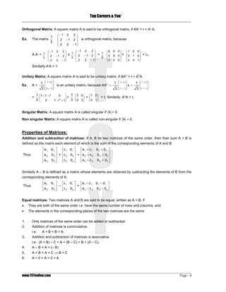
Transpose of a matrix: The transpose of a given matrix A is obtained by interchanging the rows and columns
of the matrix A. Transpose of A is denoted by A' or A'.
Thus, if A = [aij]mxn Then A' = [bij]nxm Where bij = aji
⎛1 2⎞
If A = ⎛
1 3 5⎞
Ex. ⎜
⎜ ⎟
⎟
Then A' = ⎜ 3 7 ⎟
⎜ ⎟
⎝2 7 0⎠ ⎜5
⎝ 0⎟
⎠
Properties of Transpose: Let A and B be two matrices. Then
(i) (AT)T = A
(ii) (A + B)T = AT + BT, A and B being of the same order.
(iii) (kA)T = kAT, k be any scalar (real or complex).
(iv) (AB)T = BTAT, A and B being conformable for the product AB.
Conjugate of a Matrix: The conjugate of a given matrix A is obtained by replacing the elements of A by their
corresponding complex conjugates. The conjugate of A is denoted by A .
Thus, if A = [aij]mxn then A = [ a ij]mxn
1 1 +i⎞ ⎛1 1 − i ⎞
Ex: If A = ⎛
⎜
⎜ ⎟ then A = ⎜
⎟ ⎜ ⎟
⎟
⎝3 1 −1⎠ ⎝3 1 + 1⎠
Tranjugate or Transposed Conjugate of a Matrix: The transpose conjugate of a given matrix is obtained by
interchanging the rows and columns of the matrix obtained by replacing the element of A by their
corresponding complex conjugate. The transpose conjugate of A is denoted by A* or by A θ . Thus,
A* = ( A ' ) = ( A )’
⎛ 2 3⎞
2 1+ i 0⎞ ⎜ ⎟
Ex. If A = ⎛
⎜
⎜ ⎟ then A* = ⎜1− i 2 ⎟
⎟
⎝3 2 i⎠ ⎜ 0
⎝ − i⎟
⎠
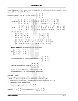
Symmetric and skew-symmetric matrices: A square matrix A = [aij] is said to be symmetric when aij = aji for
all i and j.
If aij = – aji for all i and j so that all the leading diagonal elements are zero, then the matrix is called a skew-
symmetric matrix.
Examples of symmetric and skew-symmetric matrices are respectively.
⎡a h g⎤ ⎡ 0 h − g⎤
⎢ ⎥ ⎢ ⎥
⎢h b f ⎥ and ⎢− h 0 f ⎥
⎢
⎣g f c ⎥
⎦ ⎢ g −f 0 ⎥
⎣ ⎦
Note: Every square matrix can be uniquely expressed as a sum of a symmetric and a skew-symmetric matrix
as:
A = ½ (A + A’) + ½ (A – A’).
_________________________________________________________________________________________________
www.TCYonline.com Page : 2

3. Top Careers & You
®
_________________________________________________________________________________
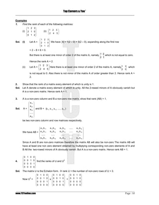
Hermitian Matrix: A square matrix A is said to be a Hermitian matrix if the transpose of the conjugate matrix
is equal to the matrix itself i.e., A* = A ⇒ a ij = aji, where A = [aij]nxn; aij ∈ C.
⎛ 3 2 + i 5i ⎞
⎛ 2 3 + 2i ⎞ ⎜ ⎟
Ex : ⎜
⎜ 3 − 2i ⎟ ⎜2 − i 0 2⎟
⎝ 7 ⎟ ⎠ ⎜− 5i
⎝ 2 7⎟ ⎠
Skew Hermitian Matrix: A square matrix A is said to be skew-Hermitian, if
A* = – A ⇒ a ij = – aji
⎛ 4i 2−i 3 ⎞
⎛ 2i 5 + 4i ⎞ ⎜ ⎟
Ex. ⎜
⎜ − 5 − 4i ⎟ ⎜− 2 + i 0 4 ⎟ are skew –Hermitian matrices.
⎝ 0 ⎟ ⎠ ⎜ −3
⎝ − 4 − 3i ⎟
⎠
Idempotent Matrix: A square matrix A, such that A2 = A is called idempotent matrix
⎛ 2 − 2 − 4⎞
⎜ ⎟
Ex. ⎜ − 1 3 4 ⎟ is idempotent because
⎜ 1 − 2 − 3⎟
⎝ ⎠
⎛ 2 − 2 − 4 ⎞ ⎛ 2 − 2 − 4 ⎞ ⎛ 4 + 2 − 4 − 4 − 6 + 4 − 8 − 8 + 12 ⎞
2 ⎜ ⎟ ⎜ ⎟ ⎜ ⎟
A = A. A = ⎜ − 1 3 4 ⎟ ⎜−1 3 4 ⎟ = ⎜− 2 − 3 + 4 2 + 9 − 8 4 + 12 − 12 ⎟
⎜ 1 − 2 − 3⎟ ⎜ 1 − 2 − 3⎟ ⎜ 2 + 2 − 3 − 2 − 6 + 6 − 4 − 8 + 9 ⎟
⎝ ⎠ ⎝ ⎠ ⎝ ⎠
⎛ 2 − 2 − 4⎞ ⎛ 2 − 2 − 4⎞ ⎛ 4 + 2 − 4 − 4 − 6 + 4 − 8 − 8 + 12 ⎞
2 ⎜ ⎟ ⎜ ⎟ ⎜ ⎟
A = A. A = ⎜ − 1 3 4 ⎟ ⎜− 1 3 4 ⎟ = ⎜− 2 − 3 + 4 2 + 9 − 8 4 + 12 − 12 ⎟
⎜ 1 − 2 − 3⎟ ⎜ 1 − 2 − 3⎟ ⎜ 2+2−3 −2−6+6 −4−8+9 ⎟
⎝ ⎠ ⎝ ⎠ ⎝ ⎠
⎛ 2 − 2 − 4⎞
⎜ ⎟
⎜− 1 3 4 ⎟= A
⎜ 1 − 2 − 3⎟
⎝ ⎠
Nilpotent Matrix: If A is a square matrix such that Am = 0, where m is a positive integer, than A is called a
nilpotent matrix. If m is the least positive integer for which Am = 0, then A is called to be nilpotent matrix of
index m.
⎛ 1 2 3 ⎞
⎜ ⎟ 2
Ex. The matrix A = ⎜ 1 2 3 ⎟ is a nilpotent matrix of index 2, because A = A . A
⎜− 1 − 2 − 3⎟
⎝ ⎠
⎛ 1 2 3 ⎞ ⎛ 1 2 3 ⎞ ⎛ 1+ 2 − 3 2+4−6 3 + 6 − 9 ⎞ ⎛0 0 0⎞
⎜ ⎟ ⎜ ⎟ ⎜ ⎟ ⎜ ⎟
⎜ 1 2 3 ⎟ × ⎜ 1 2 3 ⎟ = ⎜ 1+ 2 − 3 2+4−6 3 + 6 − 9 ⎟ = ⎜0 0 0⎟ = 0
⎜− 1 − 2 − 3⎟ ⎜− 1 − 2 − 3⎟ ⎜− 1− 2 + 3 − 2 − 2 + 6 − 3 − 6 + 9⎟ ⎜0 0 0⎟
⎝ ⎠ ⎝ ⎠ ⎝ ⎠ ⎝ ⎠
Involutory Matrix: A square matrix A such that A2 = I is called involutory matrix.
The matrix A = ⎛
1 0⎞ 2
Ex. ⎜
⎜ ⎟ is involutory because A = A . A
⎝ 0 − 1⎟
⎠
⎛ 1.1 + 0.0 1.0 + 0(−1) ⎞
= ⎛
0⎞ ⎛1 0 ⎞
= ⎛
1 1 0⎞
⎜
⎜ ⎟ × ⎜
⎟ ⎜ 0 − 1⎟
⎟
= ⎜
⎜ 0.1 + (−1).0 0.0 + (−1).(−1) ⎟
⎟ ⎜
⎜ ⎟
⎟
⎝ 0 − 1⎠ ⎝ ⎠ ⎝ ⎠ ⎝ 0 1⎠
_________________________________________________________________________________________________
www.TCYonline.com Page : 3

4. Top Careers & You
®
_________________________________________________________________________________
Orthogonal Matrix: A square matrix A is said to be orthogonal matrix, if AA' = I = A' A.
⎛−1 2 2⎞
1 ⎜ ⎟
Ex. The matrix ⎜ 2 −1 2 ⎟ is orthogonal matrix, because
3 ⎜ 2
⎝ 2 − 1⎟
⎠
⎛− 1 2 2⎞ ⎛− 1 2 2 ⎞ ⎛9 0 0⎞ ⎛1 0 0⎞
A A’ = 1 ⎜ 2 ⎟ 1 ⎜ ⎟ 1 ⎜ ⎟ ⎜ ⎟
−1 2 ⎟ x ⎜ 2 −1 2 ⎟ = ⎜0 9 0⎟ = ⎜0 1 0 ⎟ = I3.
3 ⎜ 3 ⎜ 9
⎜ 2
⎝ 2 − 1⎟
⎠ ⎝ 2 2 − 1⎟
⎠
⎜0
⎝ 0 9⎟
⎠
⎜0
⎝ 0 1⎟⎠
Similarly A'A = 1
Unitary Matrix: A square matrix A is said to be unitary matrix, if AA* = I = A*A.
1 ⎡ 1 1+i⎤ 1 ⎡ 1 1+i⎤ 1 ⎡ 1 1+i⎤
Ex. A= ⎢ ⎥ is an unitary matrix, because AA* = ⎢1−i −1⎥ x = ⎢ ⎥
3 ⎣1−i −1⎦ 3⎣ ⎦ 3 ⎣1−i −1⎦
1 ⎛1 + 1 − i 2 0 ⎞ 1 ⎛3 0⎞ ⎛ 1 0⎞
= ⎜ ⎟= ⎜ ⎟ = ⎜
⎜ 0 1⎟
= I. Similarly, A*A = I.
3 ⎜ 0
⎝ 1 − i 2 + 1⎟ 3 ⎜ 0 3 ⎟
⎠ ⎝ ⎠ ⎝
⎟
⎠
Singular Matrix: A square matrix A is called singular if A = 0.
Non singular Matrix: A square matrix A is called non-singular if A ≠ 0.
Properties of Matrices:
Addition and subtraction of matrices: If A, B be two matrices of the same order, then their sum A + B is
defined as the matrix each element of which is the sum of the corresponding elements of A and B
⎡a 1 b1 ⎤ ⎡c 1 d1 ⎤ ⎡a 1 + c 1 b 1 + d1 ⎤
⎢ ⎥ ⎢ ⎥ ⎢ ⎥
Thus ⎢a 2 b 2 ⎥ + ⎢c 2 d 2 ⎥ = ⎢a 2 + c 2 b 2 + d 2 ⎥
⎢a 3
⎣ b3 ⎥⎦ ⎢c 3 d 3 ⎥
⎣ ⎦ ⎢a 3 + c 3 b 3 + d 3 ⎥
⎣ ⎦
Similarly A – B is defined as a matrix whose elements are obtained by subtracting the elements of B from the
corresponding elements of A.
⎡a 1 b1 ⎤ ⎡c 1 d1 ⎤ ⎡a 1 − c 1 b 1 − d1 ⎤
Thus ⎢ ⎥ – ⎢ ⎥ = ⎢ ⎥
⎣a 2 b2 ⎦ ⎣c 2 d 2 ⎦ ⎣a 2 − c 2 b 2 − d 2 ⎦
Equal matrices: Two matrices A and B are said to be equal, written as A = B, if
• They are both of the same order i.e. have the same number of rows and columns, and
• The elements in the corresponding places of the two matrices are the same
1. Only matrices of the same order can be added or subtracted.
2. Addition of matrices is commutative,
i.e. A + B = B + A.
3. Addition and subtraction of matrices is associative.
i.e. (A + B) – C = A + (B – C) = B + (A – C).
4. A – B = A + (– B)
5. A+B=A+C⇒B=C
6. A+0=A=0+A
_________________________________________________________________________________________________
www.TCYonline.com Page : 4

5. Top Careers & You
®
_________________________________________________________________________________
Multiplication of matrix by a scalar: The product of a matrix A by a scalar k is a matrix whose each element
is k times the corresponding elements of A.
⎡a b c ⎤ ⎡ka kb 1 kc 1 ⎤
Thus k ⎢ 1 1 1 ⎥ = ⎢ 1 ⎥
⎣a2 b2 c 2 ⎦ ⎣ka 2 kb 2 kc 2 ⎦
The distributive law holds for such products, i.e. k (A + B) = kA + kB.
All the laws of ordinary algebra hold for the addition or subtraction of matrices and their multiplication by
scalars. Therefore
• (k + l ) A = kA + l A
• (k l ) A = k ( l A) = l (kA)
• l A = A l , l ∈ R (or C)
• k (A + B) = kA + kB
Ex: Evaluate 3A – 4B, where
⎡3 −4 6⎤ ⎡1 0 1 ⎤
A= ⎢ ⎥ and B = ⎢ ⎥
⎣5 1 7⎦ ⎣2 0 3 ⎦
⎡9 − 12 18⎤ ⎡4 0 4⎤
We have 3A = ⎢ ⎥ and 4B = ⎢ ⎥
⎣15 3 21 ⎦ ⎣8 0 12 ⎦
⎡9 − 4 − 12 − 0 18 − 4 ⎤ ⎡5 − 12 14⎤
∴ 3A – 4B = ⎢ ⎥ = ⎢ ⎥
⎣15 − 8 3−0 21 − 12⎦ ⎣7 3 9⎦
Multiplication of matrices: Two matrices can be multiplied only when the number of columns in the first is
equal to the number of rows in the second. Such matrices are said to be conformable.
⎛ 2 1 3⎞ ⎛1 − 2⎞
⎜ ⎟ ⎜ ⎟
For example, If A = ⎜ 3 −2 1 ⎟ and B = ⎜ 2 1 ⎟ , then A and B are conformable for the product AB such
⎜− 1 0 1⎟ ⎜4 − 3⎟
⎝ ⎠ ⎝ ⎠
⎛ 1⎞
that (AB)11 = (First row of A) (First column of B) = [2 1 3] ⎜ 2 ⎟ = 2*1 + 1*2 + 3*4 = 16 (AB) 12 = (First row of A)
⎜ ⎟
⎜ 4⎟
⎝ ⎠
⎛ − 2⎞ ⎛16 − 12⎞
(Second column of B) = [2 1 3] ⎜ ⎟ = 2* – 2 + 1*1 + 3 * – 3 = – 12 etc. Thus AB = ⎜ 3
⎜
⎟
− 11⎟ .
⎜ 1⎟
⎜ − 3⎟ ⎜3 −1 ⎟
⎝ ⎠ ⎝ ⎠
Properties of Matrix Multiplication:
• Matrix multiplication is associative i.e. if A, B, C are m x n, n x p and q x q matrices respectively, then (AB)
C = A (BC)
• Matrix multiplication is not always commutative AB ≠ BA
• Matrix multiplication is distributive over matrix addition i.e. A (B + C) = AB + AC where A, B, C are m x n, n
x p, n x p matrices respectively
• The product of two matrices can be the null matrix while neither of them is the null matrix.
For example, if A = ⎛
0 2⎞ ⎛ 1 0⎞ ⎛0 0⎞
⎜
⎜ ⎟ and B = ⎜
⎟ ⎜ ⎟ then AB = ⎜
⎟ ⎜ ⎟ while neither A nor B is a null matrix.
⎟
⎝0 0⎠ ⎝0 0⎠ ⎝0 0⎠
• Two matrix are said to be commute if AB = BA.
If AB = – BA, they are called Anti-commute.
_________________________________________________________________________________________________
www.TCYonline.com Page : 5

6. Top Careers & You
®
_________________________________________________________________________________
Power of a matrix: If A be a square matrix, then the product AA is defined as A2. Similarly, we define higher
powers of A. i.e. A.A2 = A3, A2. A2 = A4 etc.
⎡1 3 2⎤
⎢ ⎥
Exam. Prove that A3 – 4A2 – 3A + 11 I = 0, where A = ⎢2 0 − 1⎥ .
⎢1
⎣ 2 3⎥
⎦
⎡1 3 2⎤ ⎡1 3 2⎤ ⎡1 + 6 + 2 3 + 0 + 4 2 − 3 + 6⎤ ⎡9 7 5 ⎤
⎢ ⎥ ⎢ ⎥ ⎢ ⎥ ⎢ ⎥
A = A × A = ⎢2
2
0 − 1⎥ × ⎢2 0 − 1⎥ = ⎢2 + 0 − 1 6 + 0 − 2 4 + 0 − 3 ⎥ = ⎢1 4 1 ⎥
⎢1
⎣ 2 3⎥
⎦ ⎢1
⎣ 2 3⎥
⎦ ⎢1 + 4 + 3 3 + 0 + 6 2 − 2 + 9 ⎥
⎣ ⎦ ⎢8 9 9⎥
⎣ ⎦
⎡9 7 5 ⎤ ⎡1 3 2⎤ ⎡9 + 14 + 5 27 + 0 + 10 18 − 7 + 15 ⎤ ⎡28 37 26⎤
⎢ ⎥ ⎢ ⎥ ⎢ ⎥ ⎢ ⎥
A = A × A = ⎢1 4 1 ⎥ × ⎢2
3 2
0 − 1⎥ = ⎢1 + 8 + 1 3+0+2 2 − 4 + 3 ⎥ = ⎢10 5 1⎥
⎢8 9 9⎥
⎣ ⎦ ⎢1
⎣ 2 3⎥
⎦ ⎢8 + 18 + 9 24 + 0 + 18 16 − 9 + 27⎥
⎣ ⎦ ⎢35
⎣ 42 34 ⎥
⎦
A3 – 4A2 – 3A + 11 I
⎡28 37 26⎤ ⎡9 7 5 ⎤ ⎡1 3 2⎤ ⎡1 0 0⎤
⎢ ⎥ ⎢ ⎥ ⎢ ⎥ ⎢ ⎥
⎢10 5 1⎥ – 4 ⎢1 4 1 ⎥ – 3 ⎢2 0 − 1⎥ + 11 ⎢0 1 0⎥
⎢35
⎣ 42 34 ⎥
⎦ ⎢8 9 9⎥
⎣ ⎦ ⎢1
⎣ 2 3⎥
⎦ ⎢0 0 1⎥
⎣ ⎦
⎡28 − 36 − 3 + 11, 37 − 28 − 9 + 0, 26 − 20 − 6 + 0 ⎤ ⎡0 0 0⎤
⎢ ⎥ ⎢ ⎥
= ⎢10 − 4 − 6 − 0, 5 − 16 + 0 + 11, 1 − 4 + 3 + 0 ⎥ = ⎢0 0 0⎥ = 0
⎢35 − 32 − 3 + 0, 42 − 36 − 6 + 0,
⎣ 34 − 36 − 9 + 11⎥
⎦ ⎢0 0 0⎥
⎣ ⎦
Adjoint of A Matrix: The determinant of the square matrix
a1 b1 c 1 a1 b1 c 1
A = a2 b2 c 2 is ∆ a 2 b 2 c2
a3 b3 c3 a3 b3 c3
A 1 B 1 C1
The matrix formed by the cofactors of the elements in ∆ is A 2 B 2 C2 .
A 3 B3 C3
A1 A 2 A3
Then, the transpose of this matrix, i.e. B 1 B 2 B3
C1 C 2 C3
is called the adjoint of the matrix A and is written as Adj. A.
Thus the Adjoint of A is the transposed matrix of cofactors of A.
Inverse of a matrix:
Let A be a square matrix of order n. If there exists a matrix B, such that
A. B = B. A = I, then B is called the inverse of the matrix and denoted by A–1.
The Inverse of a Square Matrix A exists if and only if A is non-singular (i.e., det A ≠ 0).
The Inverse a Square Matrix is unique.
−1 adj A
If A is a non-singular matrix then A =
det A
⎡a b⎤ −1 1 ⎡a b⎤
Example: If A = ⎢ ⎥ is non-singular then A = ⎢ ⎥
⎣c d⎦ ad − bc ⎣c d⎦
_________________________________________________________________________________________________
www.TCYonline.com Page : 6

7. Top Careers & You
®
_________________________________________________________________________________
⎡ 2 0 ⎤ ⎡ 1 − 2⎤
Example: If A = ⎢ ⎥+⎢ ⎥ , then A + B = _______ and A – B = _____
⎣− 3 4⎦ ⎣0 4 ⎦
⎡ 2 0 ⎤ ⎡ 1 − 2⎤
Solution: A +B = ⎢ ⎥+⎢ ⎥
⎣− 3 4⎦ ⎣0 4 ⎦
⎡ 2 + 1 0 + ( −2)⎤ ⎡ 3 − 2⎤
=⎢ ⎥= ⎢ ⎥
⎣− 3 + 0 4+4 ⎦ ⎣− 3 8 ⎦
⎡ 2 0 ⎤ ⎡ 1 − 2⎤ ⎡ 2 − 1 0 − ( −2)⎤ ⎡ 3 2⎤
A −B = ⎢ ⎥+⎢ ⎥ =⎢ ⎥= ⎢ ⎥
⎣− 3 4⎦ ⎣0 4 ⎦ ⎣− 3 + 0 4−4 ⎦ ⎣− 3 0⎦
⎡1 ω ω2 ⎤
⎢ ⎥
Example: Evaluate ∆ = ⎢ ω ω2 1⎥
⎢ω2 1 ω⎥
⎣ ⎦
Operating r1 → r1 + r2 + r3 we get,
⎡1 + ω + ω2 ω + ω2 + 1 ω 2 + 1 + ω⎤
⎢ ⎥
∆=⎢ ω ω2 1 ⎥
⎢ ω2 1 ω ⎥
⎣ ⎦
⎡0 0 0⎤
⎢ ⎥
= ⎢ω ω2 1⎥ = 0 [Q (1 + ω + ω2 ) = 0]
⎢ 2
⎣ω 1 ω⎥
⎦
Example: Find the inverse of the matrix
⎡1 4⎤ ⎡3 4⎤ ⎡3 1⎤
Solution: det A = 1⎢ ⎥ − 2⎢ ⎥ + 5⎢ ⎥
⎣1 2⎦ ⎣ 1 2⎦ ⎣ 1 1⎦
= – 2 – 4 + 10 = 14
⇒ det A ≠ 0
∴ A is non – singular
Let Aij denote the co-factor of aij of the matrix A.
⎡1 4⎤
∴ A11 = ( −1)1+1 ⎢ ⎥ = −2,
⎣1 2⎦
⎡3 4⎤
A12 = ( −1)1+ 2 ⎢ ⎥ = −2,
⎣ 1 2⎦
⎡3 1⎤
A13 = ( −1)1+ 3 ⎢ ⎥ = 2,
⎣1 1⎦
⎡2 5⎤
A 21 = ( −1)2 +1 ⎢ ⎥ =1,
⎣ 1 2⎦
⎡1 2⎤
A 22 = ( −1)2 + 2 ⎢ ⎥ = 1,
⎣1 1⎦
⎡2 5 ⎤
A 31 = ( −1)3 +1 ⎢ ⎥ = 3,
⎣ 1 4⎦
⎡1 5⎤
A 32 = ( −1) 3 + 2 ⎢ ⎥ = 11,
⎣3 4⎦
_________________________________________________________________________________________________
www.TCYonline.com Page : 7

8. Top Careers & You
®
_________________________________________________________________________________
⎡ 1 2⎤
A 33 = ( −1)3 + 3 ⎢ ⎥ = −5,
⎣3 1⎦
⎡− 2 − 2 2 ⎤
⎢ ⎥
∴ Matrix of co − factors = ⎢ 1 − 3 1 ⎥
⎢ 3 11 − 5⎥
⎣ ⎦
⎡− 2 1 3 ⎤
⎢ ⎥
Adj A = ⎢− 2 − 3 11 ⎥
⎢2
⎣ 1 − 5⎥⎦
⎡− 2 1 3 ⎤
Adj A 1 ⎢ ⎥
A −1 = = ⎢− 2 − 3 11 ⎥
det A 4
⎢2
⎣ 1 − 5⎥⎦
Coshα Sinhα
Example: If A = , find A −1
Sinhα Coshα
Coshα Sinhα
Solution: det A =
Sinhα Coshα
= cos h2α – sinh2α = 1 ≠ 0. ∴ A–1 can be computed
RANK OF A MATRIX:
If we select any r rows and r columns from any matrix A, deleting all the other rows and columns, then the
determinant formed by these r × r elements is called the minor of A of order r. Clearly there will be a number of
different minors of the same order, got by deleting different rows and columns form the same matrix.
Def. A matrix is said to be of rank r when
(i) it has at least one non-zero minor of order r,
and (ii) every minor of order higher than r vanishes.
Briefly, the rank of a matrix is the largest order of any non-vanishing minor of the matrix.
If a matrix has a non-zero minor of order r, its rank is ≥ r.
If all minors of a matrix of order r + 1 are zero, its rank is ≤ r.
Note:
1. Since the rank of every non-zero matrix is ≥ 1, we agree to assign the rank, zero to every null matrix.
2. Every (r + 1) rowed minor of a matrix can be expressed as the sum of its r-rowed minors Therefore if all
the r-rowed minors of a matrix are equal to zero, then obviously all its (r + 1) rowed minors will also be
equal to zero.
Important: The following two simple results will help us very much in finding the rank of a matrix.
(i) The rank of a matrix is ≤ r , if all (r + 1)-rowed minors of the matrix vanish
(ii) The rank of a matrix is ≥ r, if there is at least one r-rowed minor of the matrix which is not equal to zero.
Examples:
⎛ 1 0 0⎞
⎜ ⎟
1. Let A = I3 = ⎜ 0 1 0 ⎟ be a unit matrix of order 3.
⎜ 0 0 1⎟
⎝ ⎠
We have A = 1 Therefore A is a non-singular matrix Hence rank A = 3.In particular, the rank of a unit
matrix of order n is n
_________________________________________________________________________________________________
www.TCYonline.com Page : 8

9. Top Careers & You
®
_________________________________________________________________________________
⎛0 0 0⎞
⎜ ⎟
2. Let A = ⎜ 0 0 0 ⎟ Since A is a null matrix, therefore rank A = 0
⎜0 0 0⎟
⎝ ⎠
⎛1 2 3⎞
⎜ ⎟
3. Let A = ⎜ 2 3 4 ⎟ We have A = 1 (6 – 8) – 2(4 – 4) + 3(4 – 3) = 2 + 1 = 3. Thus A is a non-singular
⎜ 1 2 2⎟
⎝ ⎠
Therefore rank A = 3.
⎛ 1 2 3⎞
⎜ ⎟
4. Let A = ⎜ 3 4 5 ⎟ . We have A = 1 (24 – 25) – 2 (18 – 20) + 3 (15 – 16) = 0.
⎜ 4 5 6⎟
⎝ ⎠
1 2
Therefore the rank of A is less than a 3. Now there is at least one minor of A or order 2, namely
3 4
which is not equal to zero Hence rank A = 2.
⎛3 1 2⎞
⎜ ⎟
5. Let A = ⎜ 6 2 4 ⎟ we have A = 0, since the first two columns are identical Also each 2 – rowed
⎜3 1 2⎟
⎝ ⎠
minor of A is equal to zero. But A is not a null matrix. Hence rank A = 1
⎛ 2 4 3 2⎞ 2 4
6. Let A = ⎜
⎜3 5 1 4 ⎟
⎟ Here we see that there is at least one minor of A of order 2 i.e., which is
⎝ ⎠ 3 5
not equal to zero Also there is no minor of A of order greater that 2 Hence rank of A = 2
Echelon form of matrix: A matrix A is said to be Echelon from if
(i) Every row of A which has all its entries 0 occurs below every row, which has a non-zero entry.
(ii) The first non-zero entry in each non-zero row is equal to 1.
(iii) The number of zeros before the first non-zero element in a row is less than the number of such zeros in
the next row.
Important result:
The rank of a matrix in Echelon from is equal to the number of non-zero rows of the matrix.
⎛0 1 2 3 ⎞
⎜ ⎟
Ex Find the rank of the matrix ⎜ 0 0 1 − 1⎟
⎜0 0 0 0 ⎟
⎝ ⎠
Sol. The matrix A has zero row. We see that it occurs below every non-zero row. Further the number of zero
before the first non-zero element in the first row is one. The number of zeros before the first non-zero
element in the second row it two. Thus the number of zeros before the first non-zero element in any row
is less than the number of such zeros in the next row. Thus the matrix A is in Echelon from rank A =
the number of non-zero rows of A = 2.
_________________________________________________________________________________________________
www.TCYonline.com Page : 9

10. Top Careers & You
®
_________________________________________________________________________________
Examples
1. Find the rank of each of the following matrices:
⎛ 1 2 3⎞
⎜ ⎟
(ii) ⎛
1 2 3 ⎞
(i) ⎜ 2 1 0 ⎟ ⎜
⎜ ⎟
⎟
⎜ 0 1 2⎟ ⎝2 4 5⎠
⎝ ⎠
⎛ 1 2 3⎞
Sol. (i) Let A = ⎜ 2 1 0 ⎟ We have A = 1(2 – 0) + 3(2 – 0), expanding along the first row
⎜ ⎟
⎜0 1 2⎟
⎝ ⎠
= 2 – 8 + 6 = 0.
1 2
But there is at least one minor of order 2 of the matrix A, namely which is not equal to zero.
2 1
Hence the rank A = 2.
⎛1 2 3 ⎞ 1 3
(ii) ⎜ 2 4 5 ⎟ Here there is at least one minor of order 2 of the matrix A, namely 2 5 which
Let A = ⎜ ⎟
⎝ ⎠
is not equal to 0. Also there is not minor of the matrix A of order greater than 2. Hence rank A =
2.
2. Show that the rank of a matrix every element of which is unity is 1.
Sol. Let A denote a matrix every element of which is unity. All the 2-rewed minors of A obviously vanish but
A is a non-zero matrix. Hence rank A = 1.
3. A is a non-zero column and B a non-zero row matrix, show that rank (AB) = 1.
⎛ a 11 ⎞
⎜ ⎟
⎜ a 21 ⎟
Sol. A = ⎜ a ⎟ and B = (b 11 b 12 b 13 ....... b in )
⎜ 31 ⎟
⎜ ...... ⎟
⎜ ⎟
⎝ a ml ⎠
be two non-zero column and row matrices respectively.
⎛ a 11b 11 a 11b 12 a 11b 13 ...... a 11b 1n ⎞
⎜ ⎟
We have AB = ⎜ a 21b 11 a 21b 12 a 21b 13 ...... a 21b 1n ⎟
⎜ ...... ...... ...... ...... ...... ⎟
⎜ ⎟
⎜a b a ml b 12 a ml b 13 ...... a ml b 1n ⎟
⎝ ml 11 ⎠
Since A and B are non-zero matrices therefore the matrix AB will also be non-zero The matrix AB will
have at least one non zero element obtained by multiplying corresponding non-zero elements of A and
B All the two-rowed minors of A obviously vanish. But A is a non-zero matrix. Hence rank AB = 1.
⎛0 1 0 0⎞
⎜ ⎟
4. ⎜0 0 1 0 ⎟ find the ranks of U and U2
⎜0 0 0 1⎟
⎜ ⎟
⎜0 0 0 0⎟
⎝ ⎠
Sol. The matrix U is the Echelon form. rank U = the number of non-zero rows of U = 3.
⎛0 1 0 0⎞ ⎛0 1 0 0⎞ ⎛0 0 1 0⎞
⎜ ⎟ ⎜ ⎟ ⎜ ⎟
Now U =
2 ⎜0 0 1 0⎟ x ⎜0 0 1 0⎟ = ⎜0 0 1 0⎟
⎜0 0 0 1⎟ ⎜0 0 0 1⎟ ⎜0 0 0 0⎟
⎜ ⎟ ⎜ ⎟ ⎜ ⎟
⎜0 ⎟
0 0 0⎠ ⎜0 0 0 0⎟ ⎜0 0 0 0⎟
⎝ ⎝ ⎠ ⎝ ⎠
_________________________________________________________________________________________________
www.TCYonline.com Page : 10

11. Top Careers & You
®
_________________________________________________________________________________
Elementary Operations: An elementary operation is said to be row (or column) operation if it is applied to
rows (or columns). There are three types of elementary operations:
Type 1: The interchanging of ith row (or columns) of the matrix, this operation is denoted by
Ri <--> Rj or (Ci <--> Cj) or by Rij (Cij)
Type 2: If ith row (or column) of the matrix is multiplied by scalar K(K ≠ 0), then this row (or column)
operation is denoted by Ri <--> kRj (Ci <--> Cj)
Type 3: If k times of the elements of the ith row (or column) are added to the corresponding elements of jth
row (or column), then this row (column) operation is denoted by RJ RJ or kRi (or Cj Cj + kCj
Examples:
⎛ 1 0⎞
1. If I = ⎜
⎜ ⎟ then E12 – E21 is equal to:
⎟
⎝0 1⎠
⎛01 0⎞ ⎛ − 1 − 1⎞
(a) ⎛ 0 − 1⎞
⎜ ⎟ (b) ⎜
⎜ ⎟
⎟ (c) ⎜
⎜ ⎟
⎟ (d) None of these
⎜ ⎟
⎝− 1 0 ⎠ ⎝ 0 0⎠ ⎝ − 1 − 1⎠
⎛ 1 0⎞ ⎛0 1⎞ ⎛0 1⎞
Sol. Given that = ⎜
⎜ ⎟ ⎜ 1 0⎟ R1 < ⇒ R12 E21 =
⎟ Therefore E12 = ⎜ ⎟ ⎜ 1 0⎟ , R1 <⇒ R2
⎜ ⎟
⎝0 1⎠ ⎝ ⎠ ⎝ ⎠
⎛0 1⎞ ⎛ 0 1⎞ ⎛0 0⎞
E12 – E21 = ⎜
⎜ ⎟ ⎜
⎟ ⎜ ⎟= ⎜
⎟ ⎜ ⎟ Therefore the correct answer is (b).
⎟
⎝ 1 0⎠ ⎝ − 1 0⎠ ⎝ 0 0⎠
2. If I = ⎛ 1 0 ⎞ , then 2E12 (2) + 3 E21 is equal to:
⎜ ⎟
⎜ ⎟
⎝0 1⎠
(a) ⎛ 2 7 ⎞
⎜ ⎟ (b) ⎛ 7
⎜
2⎞
⎟ (c) ⎛ 2 7 ⎞
⎜ ⎟ (d) ⎛ 4
⎜
4⎞
⎟
⎜ ⎟ ⎜2 3⎟ ⎜ ⎟ ⎜3 1⎟
⎝2 3⎠ ⎝ ⎠ ⎝3 2⎠ ⎝ ⎠
Sol. E12 = ⎛ 1 2 ⎞ R1 → R1 + 2R2 E21 = ⎛ 0
⎜ ⎟ ⎜
1⎞
⎟ , R1 ⇔ R2
⎜ ⎟ ⎜ 0⎟
⎝0 1⎠ ⎝1 ⎠
Therefore 2E12 (3) + 3E21 = 2 ⎛ 1 2 ⎞ + 3 ⎛ 0
⎜ ⎟ ⎜
1⎞
⎟ = ⎛2 7⎞ .
⎜ ⎟
⎜ ⎟ ⎜ 0⎟ ⎜ ⎟
⎝0 1⎠ ⎝1 ⎠ ⎝3 2⎠
Therefore the correct answer is (c).
Elementary matrices: An elementary matrix is that, which is obtained from a unit matrix, by subjecting it to
any of the elementary transformations.
Examples of elementary matrices obtained from
⎡1 0 0⎤ ⎡1 0 0⎤ ⎡1 0 0⎤ ⎡1 p 0 ⎤
⎢ ⎥ ⎢ ⎥ ⎢ ⎥ ⎢ ⎥
I3 = ⎢0 1 0⎥ are R23 ⎢0 0 1 ⎥ = C23; kR2 = ⎢0 k 0 ⎥ ; R1 + pR2 = ⎢0 1 0⎥
⎢0 0 1 ⎥
⎣ ⎦ ⎢0 1 0 ⎥
⎣ ⎦ ⎢0 0 1 ⎥
⎣ ⎦ ⎢0 0 1⎥
⎣ ⎦
Equivalent matrix: Two matrices A and b are said to be equivalent if one can be obtained from the other by a
sequence of elementary transformations. Two equivalent matrices have the same order and the same rank.
The symbol ~ is used for equivalence.
_________________________________________________________________________________________________
www.TCYonline.com Page : 11

12. Top Careers & You
®
_________________________________________________________________________________
IMPORTANT FACTS
1. The matrix obtained by applying a row operation on a given matrix is same as the matrix obtained by
pre-multiplication of the given matrix by the corresponding elementary matrix.
For Example: Let A = ⎛ 3
⎜
4⎞
⎟ Let us operate R12, then A ~ ⎛ 8
⎜
9⎞
⎟ ….. (1)
⎜8 9⎟ ⎜3 4⎟
⎝ ⎠ ⎝ ⎠
Now let 1 = ⎛ 1 0 ⎞ then by R12 we get elementary matrix E12 = ⎛ 0
⎜ ⎟ ⎜
1⎞
⎟ .
⎜ ⎟ ⎜ 0⎟
⎝0 1⎠ ⎝1 ⎠
Now E12. A = ⎛ 0
⎜
1⎞
⎟
⎛3
⎜
4⎞=
⎟
⎛8
⎜
9⎞
⎟
⎜1 0⎟ ⎜8 9⎟ ⎜3 4⎟
⎝ ⎠ ⎝ ⎠ ⎝ ⎠
Which is same as seen in (1).
2. The matrix obtained by applying a column operation on a given matrix is same as the matrix obtained
by post-multiplication of the given matrix by the corresponding elementary matrix.
3. The effect of a row operation on a product of two matrices is equivalent to the effect of the same row
operation applied only to pre-factor.
4. The effect of a column operation on a product of two matrices is equivalent to the effect of the same
column operation applied only to the post-factor.
SYSTEM OF LINEAR EQUATIONS
Consider the following system of m linear equations in n unknown x1, x2,….xn.
a11x 1 + a12 x 2 + ..... − a1n x n = b1 ⎫
⎪
a 21x 1 + a 22 x 2 + ..... − a 2n x n = b 2 ⎪
⎪
.......... .......... .......... .......... ............... ⎬
.......... .......... .......... .......... .................⎪
⎪
a m1x 1 + a m2 x 2 + ..... − a mn x n = b m ⎪ ⎭
The above system, of equations can be written as AX = B.
⎛ a11 a12 ....... a1n ⎞ ⎛ x1 ⎞ ⎛ b1 ⎞
⎜ ⎟ ⎜ ⎟ ⎜ ⎟
⎜ a 21 a12 ....... a1n ⎟ ⎜ x2 ⎟ ⎜ b2 ⎟
⎜ .... ...... ....... ...... ⎟ ⎜ ..... ⎟ = ⎜ ..... ⎟
⎜ ⎟ ⎜ ⎟ ⎜ ⎟
⎜a a m2 ....... a mn ⎟ ⎜x ⎟ ⎜b ⎟
⎝ m1 ⎠ ⎝ n⎠ ⎝ n⎠
If B = 0 i.e., b1 = b2 = b3….bn = 0, then the system of equations is called homogeneous
If B ≠ 0, then the system of equations is non-homogeneous.
_________________________________________________________________________________________________
www.TCYonline.com Page : 12

13. Top Careers & You
®
_________________________________________________________________________________
SOLUTION OF A NON-HOMOGENEOUS SYSTEM OF LINEAR EQUATIONS
There are three methods of solving a system of linear equations:
(i) Matrix method
(ii) Rank method
(iii) Determinant method (Cramer's Rule)
Matrix method: For the system of m-linear equations in n unknowns (variables) represented by AX = B.
(i) If |A| ≠ 0, then the system is consistent and has a unique solution given by X = A–1B.
(ii) If |A| = 0 and (adj A) B = 0, then the system is consistent and has infinitely many solutions.
(iii) If |A| = 0 and (adj A) B ≠ 0, then the system is inconsistent (no solution).
Rank method: For the system of m-linear equations in n unknowns (variables) represented by AX = B.
If m > n, then
(i) If r (A) = r (A : B) = n, then system of linear equations has a unique solution.
(ii) If r (A) = r (A : B) = r < n, then system of linear equations is consistent and has infinite number of
solutions. In fact, in this case (n – r) variables can be assigned arbitrary values.
(iii) If r (A) ≠ r (A : B), then the system of linear equations is inconsistent i.e. it has no solution.
If m < n and r (A) = r (A : B) = r, then there are infinite number of solutions.
Determinant method: For a system of 3 simultaneous linear equations in three unknowns.
(i) If D ≠ 0, then the given system of equations is consistent and has a unique solution given by
D1 D D
x= , y = 2 and z = 3
D' D D
(ii) If D = 0 and D1 = D2 = D3 = 0, then the given system of equations is consistent with infinitely
many solutions.
(iii) If D = 0 and at least one of the determinants D1, D2, D3 is non-zero, then the given system of
equations is inconsistent.
SOLUTION OF A HOMOGENEOUS SYSTEM OF LINEAR EQUATIONS
A homogeneous system of linear equations, AX = O is never inconsistent, as it always have a trivial solution
i.e. X = 0.
Matrix method:
Step I: If |A| ≠ 0, then “the system is consistent with unique solution x = y = z = 0.” (trivial solution)
Step II: If |A| = 0, then system of equations has infinitely many solutions.
To find these solutions proceed as follows:
Put z = k (any real number) and solve any two equations for x and y in terms of k. The values of
x and y so obtained with z = k give a solution of the given system of equations.
Rank method:
If r (A) = n = number of variables, then AX = O has a unique solution X = 0 i.e. x1 = x2 = … = 0. (trivial solution)
If r (A) = r < n (= number of variables), then the system of equations has an infinite number of solutions.
_________________________________________________________________________________________________
www.TCYonline.com Page : 13

14. Top Careers & You
®
_________________________________________________________________________________
EXAMPLE
⎛1 2 3 ⎞
⎜ ⎟
1. The rank of the matrix A = ⎜ 2 3 4 ⎟ is :
⎜ 4 10 18 ⎟
⎝ ⎠
(a) 0 (b) 1 (c) 2 (d) 3
⎛1 2 3 ⎞
⎜ ⎟
Sol. Let A = ⎜ 2 3 4 ⎟ Therefore
⎜ 4 10 18 ⎟
⎝ ⎠
⎛1 2 3 ⎞
⎜ ⎟
A = ⎜ 2 3 4 ⎟ = 1 (54 – 40) – 2(36 – 16) + 3 (20 – 12) = – 2 ≠ 0.
⎜ 4 10 18 ⎟
⎝ ⎠
Therefore p (A) ≥ 3…..(i). The matrix A does not posses any minor of order 4.
Therefore p(A) ≥ 3 …..(ii) From (i) and (ii) p (A) = 3. Therefore the correct answer is (d)
_________________________________________________________________________________________________
www.TCYonline.com Page : 14