The document discusses matrices and their properties. It begins by defining a matrix as an ordered rectangular array of numbers or functions. It then discusses the order of a matrix, types of matrices including column, row, square, diagonal and identity matrices. It also defines equality of matrices. The key points are that a matrix represents tabular data, its order is given by the number of rows and columns, and there are different types of matrices based on their properties.

1. 56 MATHEMATICS
The essence of Mathematics lies in its freedom. — CANTOR
3.1 Introduction
The knowledge of matrices is necessary in various branches of mathematics. Matrices
are one of the most powerful tools in mathematics. This mathematical tool simplifies
our work to a great extent when compared with other straight forward methods. The
evolution of concept of matrices is the result of an attempt to obtain compact and
simple methods of solving system of linear equations. Matrices are not only used as a
representation of the coefficients in system of linear equations, but utility of matrices
far exceeds that use. Matrix notation and operations are used in electronic spreadsheet
programs for personal computer, which in turn is used in different areas of business
and science like budgeting, sales projection, cost estimation, analysing the results of an
experiment etc. Also, many physical operations such as magnification, rotation and
reflection through a plane can be represented mathematically by matrices. Matrices
are also used in cryptography.This mathematical tool is not only used in certain branches
of sciences, but also in genetics, economics, sociology, modern psychology and industrial
management.
In this chapter, we shall find it interesting to become acquainted with the
fundamentals of matrix and matrix algebra.
3.2 Matrix
Suppose we wish to express the information that Radha has 15 notebooks. We may
express it as [15] with the understanding that the number inside [ ] is the number of
notebooks that Radha has. Now, if we have to express that Radha has 15 notebooks
and 6 pens. We may express it as [15 6] with the understanding that first number
inside [ ] is the number of notebooks while the other one is the number of pens possessed
by Radha. Let us now suppose that we wish to express the information of possession
Chapter 3
MATRICES
©
N
C
ER
T
notto
be
republishe

2. MATRICES 57
of notebooks and pens by Radha and her two friends Fauzia and Simran which
is as follows:
Radha has 15 notebooks and 6 pens,
Fauzia has 10 notebooks and 2 pens,
Simran has 13 notebooks and 5 pens.
Now this could be arranged in the tabular form as follows:
Notebooks Pens
Radha 15 6
Fauzia 10 2
Simran 13 5
and this can be expressed as
or
Radha Fauzia Simran
Notebooks 15 10 13
Pens 6 2 5
which can be expressed as:
In the first arrangement the entries in the first column represent the number of
note books possessed by Radha, Fauzia and Simran, respectively and the entries in the
second column represent the number of pens possessed by Radha, Fauzia and Simran,
©
N
C
ER
T
notto
be
republishe

3. 58 MATHEMATICS
respectively. Similarly, in the second arrangement, the entries in the first row represent
the number of notebooks possessed by Radha, Fauzia and Simran, respectively. The
entries in the second row represent the number of pens possessed by Radha, Fauzia
and Simran, respectively. An arrangement or display of the above kind is called a
matrix. Formally, we define matrix as:
Definition 1 A matrix is an ordered rectangular array of numbers or functions. The
numbers or functions are called the elements or the entries of the matrix.
We denote matrices by capital letters.The following are some examples of matrices:
5– 2
A 0 5
3 6
⎡ ⎤
⎢ ⎥
= ⎢ ⎥
⎢ ⎥
⎣ ⎦
,
1
2 3
2
B 3.5 –1 2
5
3 5
7
i
⎡ ⎤
+ −⎢ ⎥
⎢ ⎥
= ⎢ ⎥
⎢ ⎥
⎢ ⎥
⎣ ⎦
,
3
1 3
C
cos tansin 2
x x
x xx
⎡ ⎤+
= ⎢ ⎥
+⎣ ⎦
In the above examples, the horizontal lines of elements are said to constitute, rows
of the matrix and the vertical lines of elements are said to constitute, columns of the
matrix. Thus A has 3 rows and 2 columns, B has 3 rows and 3 columns while C has 2
rows and 3 columns.
3.2.1 Order of a matrix
Amatrix having m rows and n columns is called a matrix of order m × n or simply m × n
matrix (read as an m by n matrix). So referring to the above examples of matrices, we
have A as 3 × 2 matrix, B as 3 × 3 matrix and C as 2 × 3 matrix. We observe that A has
3 × 2 = 6 elements, B and C have 9 and 6 elements, respectively.
In general, an m × n matrix has the following rectangular array:
or A = [aij
]m × n
, 1≤ i ≤ m, 1≤ j ≤ n i, j ∈ N
Thus the ith
row consists of the elements ai1
, ai2
, ai3
,..., ain
, while the jth
column
consists of the elements a1j
, a2j
, a3j
,..., amj
,
In general aij
, is an element lying in the ith
row and jth
column. We can also call
it as the (i, j)th
element of A. The number of elements in an m × n matrix will be
equal to mn.
©
N
C
ER
T
notto
be
republishe

4. MATRICES 59
Note In this chapter
1. We shall follow the notation, namelyA= [aij
]m × n
to indicate thatAis a matrix
of order m × n.
2. We shall consider only those matrices whose elements are real numbers or
functions taking real values.
We can also represent any point (x, y) in a plane by a matrix (column or row) as
x
y
⎡ ⎤
⎢ ⎥
⎣ ⎦
(or [x, y]). For example point P(0, 1) as a matrix representation may be given as
0
P
1
⎡ ⎤
= ⎢ ⎥
⎣ ⎦
or [0 1].
Observe that in this way we can also express the vertices of a closed rectilinear
figure in the form of a matrix. For example, consider a quadrilateral ABCD with vertices
A (1, 0), B (3, 2), C (1, 3), D (–1, 2).
Now, quadrilateral ABCD in the matrix form, can be represented as
2 4
A B C D
1 3 1 1
X
0 2 3 2 ×
−⎡ ⎤
= ⎢ ⎥
⎣ ⎦
or
4 2
A 1 0
B 3 2
Y
C 1 3
D 1 2 ×
⎡ ⎤
⎢ ⎥
⎢ ⎥=
⎢ ⎥
⎢ ⎥
−⎣ ⎦
Thus, matrices can be used as representation of vertices of geometrical figures in
a plane.
Now, let us consider some examples.
Example 1 Consider the following information regarding the number of men and women
workers in three factories I, II and III
Men workers Women workers
I 30 25
II 25 31
III 27 26
Represent the above information in the form of a 3 × 2 matrix. What does the entry
in the third row and second column represent?
©
N
C
ER
T
notto
be
republishe

5. 60 MATHEMATICS
Solution The information is represented in the form of a 3 × 2 matrix as follows:
30 25
A 25 31
27 26
⎡ ⎤
⎢ ⎥= ⎢ ⎥
⎢ ⎥⎣ ⎦
The entry in the third row and second column represents the number of women
workers in factory III.
Example 2 If a matrix has 8 elements, what are the possible orders it can have?
Solution We know that if a matrix is of order m × n, it has mn elements. Thus, to find
all possible orders of a matrix with 8 elements, we will find all ordered pairs of natural
numbers, whose product is 8.
Thus, all possible ordered pairs are (1, 8), (8, 1), (4, 2), (2, 4)
Hence, possible orders are 1 × 8, 8 ×1, 4 × 2, 2 × 4
Example 3 Construct a 3 × 2 matrix whose elements are given by
1
| 3 |
2
ija i j= − .
Solution In general a 3 × 2 matrix is given by
11 12
21 22
31 32
A
a a
a a
a a
⎡ ⎤
⎢ ⎥= ⎢ ⎥
⎢ ⎥⎣ ⎦
.
Now
1
| 3 |
2
ija i j= − , i = 1, 2, 3 and j = 1, 2.
Therefore 11
1
|1 3 1| 1
2
a = − × = 12
1 5
|1 3 2|
2 2
a = − × =
21
1 1
| 2 3 1|
2 2
a = − × = 22
1
| 2 3 2| 2
2
a = − × =
31
1
|3 3 1| 0
2
a = − × = 32
1 3
|3 3 2|
2 2
a = − × =
Hence the required matrix is given by
5
1
2
1
A 2
2
3
0
2
⎡ ⎤
⎢ ⎥
⎢ ⎥
= ⎢ ⎥
⎢ ⎥
⎢ ⎥
⎣ ⎦
.
©
N
C
ER
T
notto
be
republishe

6. MATRICES 61
3.3 Types of Matrices
In this section, we shall discuss different types of matrices.
(i) Column matrix
A matrix is said to be a column matrix if it has only one column.
For example,
0
3
A 1
1/ 2
⎡ ⎤
⎢ ⎥
⎢ ⎥
⎢ ⎥= −
⎢ ⎥
⎢ ⎥⎣ ⎦
is a column matrix of order 4 × 1.
In general, A = [aij
] m × 1
is a column matrix of order m × 1.
(ii) Row matrix
A matrix is said to be a row matrix if it has only one row.
For example,
1 4
1
B 5 2 3
2 ×
⎡ ⎤
= −⎢ ⎥⎣ ⎦
is a row matrix.
In general, B = [bij
] 1 × n
is a row matrix of order 1 × n.
(iii) Square matrix
A matrix in which the number of rows are equal to the number of columns, is
said to be a square matrix. Thus an m × n matrix is said to be a square matrix if
m = n and is known as a square matrix of order ‘n’.
For example
3 1 0
3
A 3 2 1
2
4 3 1
−⎡ ⎤
⎢ ⎥
⎢ ⎥=
⎢ ⎥
⎢ ⎥−⎣ ⎦
is a square matrix of order 3.
In general, A = [aij
] m × m
is a square matrix of order m.
Note If A = [aij
] is a square matrix of order n, then elements (entries) a11
, a22
, ..., ann
are said to constitute the diagonal, of the matrix A. Thus, if
1 3 1
A 2 4 1
3 5 6
−⎡ ⎤
⎢ ⎥= −⎢ ⎥
⎢ ⎥⎣ ⎦
.
Then the elements of the diagonal of A are 1, 4, 6.
©
N
C
ER
T
notto
be
republishe

7. 62 MATHEMATICS
(iv) Diagonal matrix
A square matrix B = [bij
] m × m
is said to be a diagonal matrix if all its non
diagonal elements are zero, that is a matrix B = [bij
] m × m
is said to be a diagonal
matrix if bij
= 0, when i ≠ j.
For example, A = [4],
1 0
B
0 2
−⎡ ⎤
= ⎢ ⎥
⎣ ⎦
,
1.1 0 0
C 0 2 0
0 0 3
−⎡ ⎤
⎢ ⎥= ⎢ ⎥
⎢ ⎥⎣ ⎦
, are diagonal matrices
of order 1, 2, 3, respectively.
(v) Scalar matrix
A diagonal matrix is said to be a scalar matrix if its diagonal elements are equal,
that is, a square matrix B = [bij
] n × n
is said to be a scalar matrix if
bij
= 0, when i ≠ j
bij
= k, when i = j, for some constant k.
For example
A = [3],
1 0
B
0 1
−⎡ ⎤
= ⎢ ⎥−⎣ ⎦
,
3 0 0
C 0 3 0
0 0 3
⎡ ⎤
⎢ ⎥
= ⎢ ⎥
⎢ ⎥
⎣ ⎦
are scalar matrices of order 1, 2 and 3, respectively.
(vi) Identity matrix
A square matrix in which elements in the diagonal are all 1 and rest are all zero
is called an identity matrix. In other words, the square matrix A = [aij
] n × n
is an
identity matrix, if
1 if
0 if
ij
i j
a
i j
=⎧
= ⎨
≠⎩
.
We denote the identity matrix of order n by In
. When order is clear from the
context, we simply write it as I.
For example [1],
1 0
0 1
⎡ ⎤
⎢ ⎥
⎣ ⎦
,
1 0 0
0 1 0
0 0 1
⎡ ⎤
⎢ ⎥
⎢ ⎥
⎢ ⎥⎣ ⎦
are identity matrices of order 1, 2 and 3,
respectively.
Observe that a scalar matrix is an identity matrix when k = 1. But every identity
matrix is clearly a scalar matrix.
©
N
C
ER
T
notto
be
republishe

8. MATRICES 63
(vii) Zero matrix
A matrix is said to be zero matrix or null matrix if all its elements are zero.
For example, [0],
0 0
0 0
⎡ ⎤
⎢ ⎥
⎣ ⎦
,
0 0 0
0 0 0
⎡ ⎤
⎢ ⎥
⎣ ⎦
, [0, 0] are all zero matrices. We denote
zero matrix by O. Its order will be clear from the context.
3.3.1 Equality of matrices
Definition 2 Two matrices A = [aij
] and B = [bij
] are said to be equal if
(i) they are of the same order
(ii) each element of A is equal to the corresponding element of B, that is aij
= bij
for
all i and j.
For example,
2 3 2 3
and
0 1 0 1
⎡ ⎤ ⎡ ⎤
⎢ ⎥ ⎢ ⎥
⎣ ⎦ ⎣ ⎦
are equal matrices but
3 2 2 3
and
0 1 0 1
⎡ ⎤ ⎡ ⎤
⎢ ⎥ ⎢ ⎥
⎣ ⎦ ⎣ ⎦
are
not equal matrices. Symbolically, if two matrices A and B are equal, we write A = B.
If
1.5 0
2 6
3 2
x y
z a
b c
−⎡ ⎤⎡ ⎤
⎢ ⎥⎢ ⎥ = ⎢ ⎥⎢ ⎥
⎢ ⎥⎢ ⎥⎣ ⎦ ⎣ ⎦
, then x = – 1.5, y = 0, z = 2, a = 6 , b = 3, c = 2
Example 4 If
3 4 2 7 0 6 3 2
6 1 0 6 3 2 2
3 21 0 2 4 21 0
x z y y
a c
b b
+ + − −⎡ ⎤ ⎡ ⎤
⎢ ⎥ ⎢ ⎥− − = − − +⎢ ⎥ ⎢ ⎥
⎢ ⎥ ⎢ ⎥− − + −⎣ ⎦ ⎣ ⎦
Find the values of a, b, c, x, y and z.
Solution As the given matrices are equal, therefore, their corresponding elements
must be equal. Comparing the corresponding elements, we get
x + 3 = 0, z + 4 = 6, 2y – 7 = 3y – 2
a – 1 = – 3, 0 = 2c + 2 b – 3 = 2b + 4,
Simplifying, we get
a = – 2, b = – 7, c = – 1, x = – 3, y = –5, z = 2
Example 5 Find the values of a, b, c, and d from the following equation:
2 2 4 3
5 4 3 11 24
a b a b
c d c d
+ − −⎡ ⎤ ⎡ ⎤
=⎢ ⎥ ⎢ ⎥− +⎣ ⎦ ⎣ ⎦
©
N
C
ER
T
notto
be
republishe

9. 64 MATHEMATICS
Solution By equality of two matrices, equating the corresponding elements, we get
2a + b = 4 5c – d = 11
a – 2b = – 3 4c + 3d = 24
Solving these equations, we get
a = 1, b = 2, c = 3 and d = 4
EXERCISE 3.1
1. In the matrix
2 5 19 7
5
A 35 2 12
2
173 1 5
⎡ ⎤−
⎢ ⎥
⎢ ⎥= −
⎢ ⎥
⎢ ⎥
−⎣ ⎦
, write:
(i) The order of the matrix, (ii) The number of elements,
(iii) Write the elements a13
, a21
, a33
, a24
, a23
.
2. If a matrix has 24 elements, what are the possible orders it can have? What, if it
has 13 elements?
3. If a matrix has 18 elements, what are the possible orders it can have? What, if it
has 5 elements?
4. Construct a 2 × 2 matrix, A = [aij
], whose elements are given by:
(i)
2
( )
2
ij
i j
a
+
= (ii) ij
i
a
j
= (iii)
2
( 2 )
2
ij
i j
a
+
=
5. Construct a 3 × 4 matrix, whose elements are given by:
(i)
1
| 3 |
2
ija i j= − + (ii) 2ija i j= −
6. Find the values of x, y and z from the following equations:
(i)
4 3
5 1 5
y z
x
⎡ ⎤ ⎡ ⎤
=⎢ ⎥ ⎢ ⎥
⎣ ⎦ ⎣ ⎦
(ii)
2 6 2
5 5 8
x y
z xy
+⎡ ⎤ ⎡ ⎤
=⎢ ⎥ ⎢ ⎥+⎣ ⎦ ⎣ ⎦
(iii)
9
5
7
x y z
x z
y z
+ +⎡ ⎤ ⎡ ⎤
⎢ ⎥ ⎢ ⎥+ =⎢ ⎥ ⎢ ⎥
⎢ ⎥ ⎢ ⎥+⎣ ⎦ ⎣ ⎦
7. Find the value of a, b, c and d from the equation:
2 1 5
2 3 0 13
a b a c
a b c d
− + −⎡ ⎤ ⎡ ⎤
=⎢ ⎥ ⎢ ⎥− +⎣ ⎦ ⎣ ⎦
©
N
C
ER
T
notto
be
republishe

10. MATRICES 65
8. A = [aij
]m × n
is a square matrix, if
(A) m < n (B) m > n (C) m = n (D) None of these
9. Which of the given values of x and y make the following pair of matrices equal
3 7 5
1 2 3
x
y x
+⎡ ⎤
⎢ ⎥+ −⎣ ⎦
,
0 2
8 4
y −⎡ ⎤
⎢ ⎥
⎣ ⎦
(A)
1
, 7
3
x y
−
= = (B) Not possible to find
(C) y = 7,
2
3
x
−
= (D)
1 2
,
3 3
x y
10. The number of all possible matrices of order 3 × 3 with each entry 0 or 1 is:
(A) 27 (B) 18 (C) 81 (D) 512
3.4 Operations on Matrices
In this section, we shall introduce certain operations on matrices, namely, addition of
matrices, multiplication of a matrix by a scalar, difference and multiplication of matrices.
3.4.1 Addition of matrices
Suppose Fatima has two factories at places A and B. Each factory produces sport
shoes for boys and girls in three different price categories labelled 1, 2 and 3. The
quantities produced by each factory are represented as matrices given below:
Suppose Fatima wants to know the total production of sport shoes in each price
category. Then the total production
In category 1 : for boys (80 + 90), for girls (60 + 50)
In category 2 : for boys (75 + 70), for girls (65 + 55)
In category 3 : for boys (90 + 75), for girls (85 + 75)
This can be represented in the matrix form as
80 90 60 50
75 70 65 55
90 75 85 75
+ +⎡ ⎤
⎢ ⎥+ +⎢ ⎥
⎢ ⎥+ +⎣ ⎦
.
©
N
C
ER
T
notto
be
republishe

11. 66 MATHEMATICS
This new matrix is the sum of the above two matrices. We observe that the sum of
two matrices is a matrix obtained by adding the corresponding elements of the given
matrices. Furthermore, the two matrices have to be of the same order.
Thus, if
11 12 13
21 22 23
A
a a a
a a a
⎡ ⎤
= ⎢ ⎥
⎣ ⎦
is a 2 × 3 matrix and
11 12 13
21 22 23
B
b b b
b b b
⎡ ⎤
= ⎢ ⎥
⎣ ⎦
is another
2×3 matrix. Then, we define
11 11 12 12 13 13
21 21 22 22 23 23
A + B
a b a b a b
a b a b a b
+ + +⎡ ⎤
= ⎢ ⎥
+ + +⎣ ⎦
.
In general, if A = [aij
] and B = [bij
] are two matrices of the same order, say m × n.
Then, the sum of the two matrices A and B is defined as a matrix C = [cij
]m × n
, where
cij
= aij
+ bij
, for all possible values of i and j.
Example 6 Given
3 1 1
A
2 3 0
⎡ ⎤−
= ⎢ ⎥
⎣ ⎦
and
2 5 1
B 1
2 3
2
⎡ ⎤
⎢ ⎥=
⎢ ⎥−
⎢ ⎥⎣ ⎦
, find A + B
Since A, B are of the same order 2 × 3. Therefore, addition of A and B is defined
and is given by
2 3 1 5 1 1 2 3 1 5 0
A+B 1 1
2 2 3 3 0 0 6
2 2
⎡ ⎤ ⎡ ⎤+ + − + +
⎢ ⎥ ⎢ ⎥= =
⎢ ⎥ ⎢ ⎥− + +
⎢ ⎥ ⎢ ⎥⎣ ⎦ ⎣ ⎦
Note
1. We emphasise that if A and B are not of the same order, then A + B is not
defined. For example if
2 3
A
1 0
⎡ ⎤
= ⎢ ⎥
⎣ ⎦
,
1 2 3
B ,
1 0 1
⎡ ⎤
= ⎢ ⎥
⎣ ⎦
then A + B is not defined.
2. We may observe that addition of matrices is an example of binary operation
on the set of matrices of the same order.
3.4.2 Multiplication of a matrix by a scalar
Now suppose that Fatima has doubled the production at a factory A in all categories
(refer to 3.4.1).
©
N
C
ER
T
notto
be
republishe

12. MATRICES 67
Previously quantities (in standard units) produced by factory A were
Revised quantities produced by factory A are as given below:
Boys Girls
2 80 2 601
2 2 75 2 65
3 2 90 2 85
× ×⎡ ⎤
⎢ ⎥× ×⎢ ⎥
⎢ ⎥× ×⎣ ⎦
This can be represented in the matrix form as
160 120
150 130
180 170
⎡ ⎤
⎢ ⎥
⎢ ⎥
⎢ ⎥⎣ ⎦
. We observe that
the new matrix is obtained by multiplying each element of the previous matrix by 2.
In general, we may define multiplication of a matrix by a scalar as follows: if
A = [aij
] m × n
is a matrix and k is a scalar, then kA is another matrix which is obtained
by multiplying each element of A by the scalar k.
In other words, kA = k[aij
]m × n
= [k (aij
)] m × n
, that is, (i, j)th
element of kA is kaij
for all possible values of i and j.
For example, if A =
3 1 1.5
5 7 3
2 0 5
⎡ ⎤
⎢ ⎥
−⎢ ⎥
⎢ ⎥
⎣ ⎦
, then
3A =
3 1 1.5 9 3 4.5
3 5 7 3 3 5 21 9
2 0 5 6 0 15
⎡ ⎤ ⎡ ⎤
⎢ ⎥ ⎢ ⎥
− = −⎢ ⎥ ⎢ ⎥
⎢ ⎥ ⎢ ⎥
⎣ ⎦ ⎣ ⎦
Negative of a matrix The negative of a matrix is denoted by – A. We define
–A = (– 1) A.
©
N
C
ER
T
notto
be
republishe

13. 68 MATHEMATICS
For example, let A =
3 1
5 x
⎡ ⎤
⎢ ⎥−⎣ ⎦
, then – A is given by
– A = (– 1)
3 1 3 1
A ( 1)
5 5x x
− −⎡ ⎤ ⎡ ⎤
= − =⎢ ⎥ ⎢ ⎥− −⎣ ⎦ ⎣ ⎦
Difference of matrices If A = [aij
], B = [bij
] are two matrices of the same order,
say m × n, then difference A – B is defined as a matrix D = [dij
], where dij
= aij
– bij
,
for all value of i and j. In other words, D =A– B =A+ (–1) B, that is sum of the matrix
A and the matrix – B.
Example 7 If
1 2 3 3 1 3
A and B
2 3 1 1 0 2
−⎡ ⎤ ⎡ ⎤
= =⎢ ⎥ ⎢ ⎥−⎣ ⎦ ⎣ ⎦
, then find 2A – B.
Solution We have
2A – B =
1 2 3 3 1 3
2
2 3 1 1 0 2
=
2 4 6 3 1 3
4 6 2 1 0 2
− −⎡ ⎤ ⎡ ⎤
+⎢ ⎥ ⎢ ⎥−⎣ ⎦ ⎣ ⎦
=
2 3 4 1 6 3 1 5 3
4 1 6 0 2 2 5 6 0
− + − −⎡ ⎤ ⎡ ⎤
=⎢ ⎥ ⎢ ⎥+ + −⎣ ⎦ ⎣ ⎦
3.4.3 Properties of matrix addition
The addition of matrices satisfy the following properties:
(i) Commutative Law If A = [aij
], B = [bij
] are matrices of the same order, say
m × n, then A + B = B + A.
Now A + B = [aij
] + [bij
] = [aij
+ bij
]
= [bij
+ aij
] (addition of numbers is commutative)
= ([bij
] + [aij
]) = B + A
(ii) Associative Law For any three matrices A = [aij
], B = [bij
], C = [cij
] of the
same order, say m × n, (A + B) + C = A + (B + C).
Now (A + B) + C = ([aij
] + [bij
]) + [cij
]
= [aij
+ bij
] + [cij
] = [(aij
+ bij
) + cij
]
= [aij
+ (bij
+ cij
)] (Why?)
= [aij
] + [(bij
+ cij
)] = [aij
] + ([bij
] + [cij
]) = A + (B + C)
©
N
C
ER
T
notto
be
republishe

14. MATRICES 69
(iii) Existence of additive identity Let A = [aij
] be an m × n matrix and
O be an m × n zero matrix, then A + O = O + A = A. In other words, O is the
additive identity for matrix addition.
(iv) The existence of additive inverse Let A = [aij
]m × n
be any matrix, then we
have another matrix as – A = [– aij
]m × n
such that A + (– A) = (– A) + A= O. So
– A is the additive inverse of A or negative of A.
3.4.4 Properties of scalar multiplication of a matrix
If A = [aij
] and B = [bij
] be two matrices of the same order, say m × n, and k and l are
scalars, then
(i) k(A +B) = k A + kB, (ii) (k + l)A = k A + l A
(ii) k (A + B) = k ([aij
] + [bij
])
= k [aij
+ bij
] = [k (aij
+ bij
)] = [(k aij
) + (k bij
)]
= [k aij
] + [k bij
] = k [aij
] + k [bij
] = kA + kB
(iii) ( k + l) A = (k + l) [aij
]
= [(k + l) aij
] + [k aij
] + [l aij
] = k [aij
] + l [aij
] = k A + l A
Example 8 If
8 0 2 2
A 4 2 and B 4 2
3 6 5 1
−⎡ ⎤ ⎡ ⎤
⎢ ⎥ ⎢ ⎥= − =⎢ ⎥ ⎢ ⎥
⎢ ⎥ ⎢ ⎥−⎣ ⎦ ⎣ ⎦
, then find the matrix X, such that
2A + 3X = 5B.
Solution We have 2A + 3X = 5B
or 2A + 3X – 2A = 5B – 2A
or 2A – 2A + 3X = 5B – 2A (Matrix addition is commutative)
or O + 3X = 5B – 2A (– 2A is the additive inverse of 2A)
or 3X = 5B – 2A (O is the additive identity)
or X =
1
3
(5B – 2A)
or
2 2 8 0
1
X 5 4 2 2 4 2
3
5 1 3 6
⎛ ⎞−⎡ ⎤ ⎡ ⎤
⎜ ⎟⎢ ⎥ ⎢ ⎥= − −⎜ ⎟⎢ ⎥ ⎢ ⎥
⎜ ⎟⎢ ⎥ ⎢ ⎥−⎣ ⎦ ⎣ ⎦⎝ ⎠
=
10 10 16 0
1
20 10 8 4
3
25 5 6 12
⎛ ⎞− −⎡ ⎤ ⎡ ⎤
⎜ ⎟⎢ ⎥ ⎢ ⎥+ −⎜ ⎟⎢ ⎥ ⎢ ⎥
⎜ ⎟⎢ ⎥ ⎢ ⎥− − −⎣ ⎦ ⎣ ⎦⎝ ⎠
©
N
C
ER
T
notto
be
republishe

15. 70 MATHEMATICS
=
10 16 10 0
1
20 8 10 4
3
25 6 5 12
− − +⎡ ⎤
⎢ ⎥− +⎢ ⎥
⎢ ⎥− − −⎣ ⎦
=
6 10
1
12 14
3
31 7
− −⎡ ⎤
⎢ ⎥
⎢ ⎥
⎢ ⎥− −⎣ ⎦
=
10
2
3
14
4
3
31 7
3 3
−⎡ ⎤
−⎢ ⎥
⎢ ⎥
⎢ ⎥
⎢ ⎥
⎢ ⎥
− −⎢ ⎥
⎢ ⎥⎣ ⎦
Example 9 Find X and Y, if
5 2
X Y
0 9
⎡ ⎤
+ = ⎢ ⎥
⎣ ⎦
and
3 6
X Y
0 1
⎡ ⎤
− = ⎢ ⎥−⎣ ⎦
.
Solution We have ( ) ( )
5 2 3 6
X Y X Y
0 9 0 1
⎡ ⎤ ⎡ ⎤
+ + − = +⎢ ⎥ ⎢ ⎥−⎣ ⎦ ⎣ ⎦
.
or (X + X) + (Y – Y) =
8 8
0 8
⎡ ⎤
⎢ ⎥
⎣ ⎦
⇒
8 8
2X
0 8
⎡ ⎤
= ⎢ ⎥
⎣ ⎦
or X =
8 8 4 41
0 8 0 42
⎡ ⎤ ⎡ ⎤
=⎢ ⎥ ⎢ ⎥
⎣ ⎦ ⎣ ⎦
Also (X + Y) – (X – Y) =
5 2 3 6
0 9 0 1
⎡ ⎤ ⎡ ⎤
−⎢ ⎥ ⎢ ⎥−⎣ ⎦ ⎣ ⎦
or (X – X) + (Y + Y) =
5 3 2 6
0 9 1
− −⎡ ⎤
⎢ ⎥+⎣ ⎦
⇒
2 4
2Y
0 10
−⎡ ⎤
= ⎢ ⎥
⎣ ⎦
or Y =
2 4 1 21
0 10 0 52
− −⎡ ⎤ ⎡ ⎤
=⎢ ⎥ ⎢ ⎥
⎣ ⎦ ⎣ ⎦
Example 10 Find the values of x and y from the following equation:
5 3 4
2
7 3 1 2
x
y
−⎡ ⎤ ⎡ ⎤
+⎢ ⎥ ⎢ ⎥−⎣ ⎦ ⎣ ⎦
=
7 6
15 14
⎡ ⎤
⎢ ⎥
⎣ ⎦
Solution We have
5 3 4
2
7 3 1 2
x
y
−⎡ ⎤ ⎡ ⎤
+⎢ ⎥ ⎢ ⎥−⎣ ⎦ ⎣ ⎦
=
7 6
15 14
⎡ ⎤
⎢ ⎥
⎣ ⎦
⇒
2 10 3 4 7 6
14 2 6 1 2 15 14
x
y
−⎡ ⎤ ⎡ ⎤ ⎡ ⎤
+ =⎢ ⎥ ⎢ ⎥ ⎢ ⎥−⎣ ⎦ ⎣ ⎦ ⎣ ⎦
©
N
C
ER
T
notto
be
republishe

16. MATRICES 71
or
2 3 10 4
14 1 2 6 2
x
y
+ −⎡ ⎤
⎢ ⎥+ − +⎣ ⎦
=
7 6
15 14
⎡ ⎤
⎢ ⎥
⎣ ⎦
⇒
2 3 6 7 6
15 2 4 15 14
x
y
+⎡ ⎤ ⎡ ⎤
=⎢ ⎥ ⎢ ⎥−⎣ ⎦ ⎣ ⎦
or 2x + 3 = 7 and 2y – 4 = 14 (Why?)
or 2x = 7 – 3 and 2y = 18
or x =
4
2
and y =
18
2
i.e. x = 2 and y = 9.
Example 11 Two farmers Ramkishan and Gurcharan Singh cultivates only three
varieties of rice namely Basmati, Permal and Naura. The sale (in Rupees) of these
varieties of rice by both the farmers in the month of September and October are given
by the following matrices A and B.
(i) Find the combined sales in September and October for each farmer in each
variety.
(ii) Find the decrease in sales from September to October.
(iii) If both farmers receive 2% profit on gross sales, compute the profit for each
farmer and for each variety sold in October.
Solution
(i) Combined sales in September and October for each farmer in each variety is
given by
©
N
C
ER
T
notto
be
republishe

17. 72 MATHEMATICS
(ii) Change in sales from September to October is given by
(iii) 2% of B =
2
B
100
× = 0.02 × B
= 0.02
=
Thus, in October Ramkishan receives Rs 100, Rs 200 and Rs 120 as profit in the
sale of each variety of rice, respectively, and Grucharan Singh receives profit of Rs
400, Rs 200 and Rs 200 in the sale of each variety of rice, respectively.
3.4.5 Multiplication of matrices
Suppose Meera and Nadeem are two friends. Meera wants to buy 2 pens and 5 story
books, while Nadeem needs 8 pens and 10 story books. They both go to a shop to
enquire about the rates which are quoted as follows:
Pen – Rs 5 each, story book – Rs 50 each.
How much money does each need to spend? Clearly, Meera needs Rs (5 × 2 + 50 × 5)
that is Rs 260, while Nadeem needs (8 × 5 + 50 × 10) Rs, that is Rs 540. In terms of
matrix representation, we can write the above information as follows:
Requirements Prices per piece (in Rupees) Money needed (in Rupees)
2 5
8 10
⎡ ⎤
⎢ ⎥
⎣ ⎦
5
50
⎡ ⎤
⎢ ⎥
⎣ ⎦
5 2 5 50 260
8 5 10 50 540
× + ×⎡ ⎤ ⎡ ⎤
=⎢ ⎥ ⎢ ⎥× + ×⎣ ⎦ ⎣ ⎦
Suppose that they enquire about the rates from another shop, quoted as follows:
pen – Rs 4 each, story book – Rs 40 each.
Now, the money required by Meera and Nadeem to make purchases will be
respectively Rs (4 × 2 + 40 × 5) = Rs 208 and Rs (8 × 4 + 10 × 40) = Rs 432
©
N
C
ER
T
notto
be
republishe

18. MATRICES 73
Again, the above information can be represented as follows:
Requirements Prices per piece (in Rupees) Money needed (in Rupees)
2 5
8 10
⎡ ⎤
⎢ ⎥
⎣ ⎦
4
40
⎡ ⎤
⎢ ⎥
⎣ ⎦
4 2 40 5 208
8 4 10 4 0 432
× + ×⎡ ⎤ ⎡ ⎤
=⎢ ⎥ ⎢ ⎥× + ×⎣ ⎦ ⎣ ⎦
Now, the information in both the cases can be combined and expressed in terms of
matrices as follows:
Requirements Prices per piece (in Rupees) Money needed (in Rupees)
2 5
8 10
⎡ ⎤
⎢ ⎥
⎣ ⎦
5 4
50 40
⎡ ⎤
⎢ ⎥
⎣ ⎦
5 2 5 50 4 2 40 5
8 5 10 5 0 8 4 10 4 0
× + × × + ×⎡ ⎤
⎢ ⎥× + × × + ×⎣ ⎦
=
260 208
540 432
⎡ ⎤
⎢ ⎥
⎣ ⎦
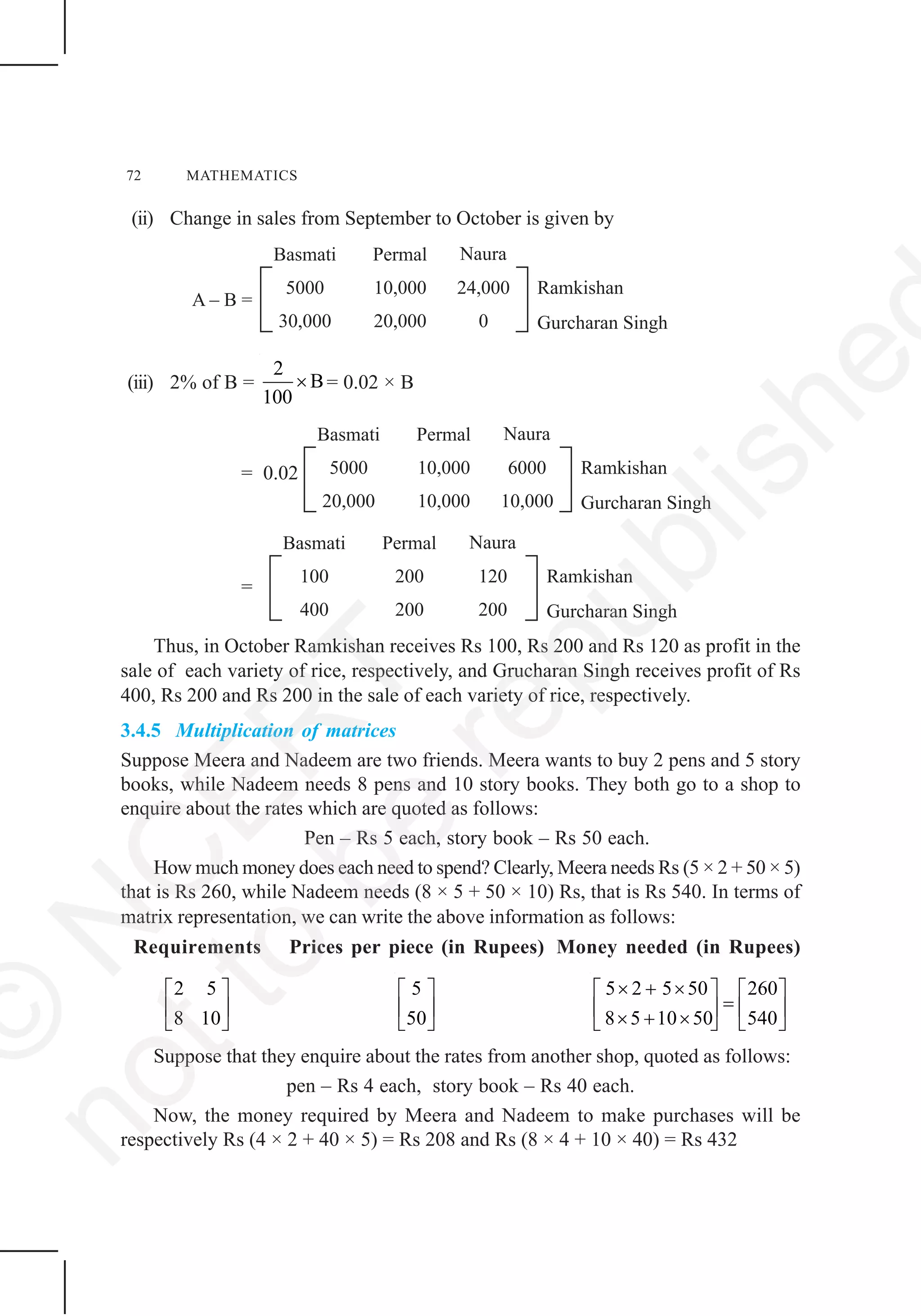
The above is an example of multiplication of matrices. We observe that, for
multiplication of two matricesAand B, the number of columns inAshould be equal to
the number of rows in B. Furthermore for getting the elements of the product matrix,
we take rows of A and columns of B, multiply them element-wise and take the sum.
Formally, we define multiplication of matrices as follows:
The product of two matrices A and B is defined if the number of columns of A is
equal to the number of rows of B. Let A = [aij
] be an m × n matrix and B = [bjk
] be an
n × p matrix. Then the product of the matrices A and B is the matrix C of order m × p.
To get the (i, k)th
element cik
of the matrix C, we take the ith
row of A and kth
column
of B, multiply them elementwise and take the sum of all these products. In other words,
if A = [aij
]m × n
, B = [bjk
]n × p
, then the ith
row of A is [ai1
ai2
... ain
] and the kth
column of
B is
1
2
.
.
.
k
k
nk
b
b
b
⎡ ⎤
⎢ ⎥
⎢ ⎥
⎢ ⎥
⎢ ⎥
⎢ ⎥
⎣ ⎦
, then cik
= ai1
b1k
+ ai2
b2k
+ ai3
b3k
+ ... + ain
bnk
=
1
n
ij jk
j
a b
=
∑ .
The matrix C = [cik
]m × p
is the product of A and B.
For example, if
1 1 2
C
0 3 4
−⎡ ⎤
= ⎢ ⎥
⎣ ⎦
and
2 7
1D 1
5 4
⎡ ⎤
⎢ ⎥= −⎢ ⎥
⎢ ⎥−⎣ ⎦
, then the product CD is defined
©
N
C
ER
T
notto
be
republishe

19. 74 MATHEMATICS
and is given by
2 7
1 1 2
CD 1 1
0 3 4
5 4
⎡ ⎤
−⎡ ⎤ ⎢ ⎥= −⎢ ⎥ ⎢ ⎥
⎣ ⎦ ⎢ ⎥−⎣ ⎦
. This is a 2 × 2 matrix in which each
entry is the sum of the products across some row of C with the corresponding entries
down some column of D. These four computations are
Thus
13 2
CD
17 13
−⎡ ⎤
= ⎢ ⎥−⎣ ⎦
Example 12 Find AB, if
6 9 2 6 0
A and B
2 3 7 9 8
⎡ ⎤ ⎡ ⎤
= =⎢ ⎥ ⎢ ⎥
⎣ ⎦ ⎣ ⎦
.
Solution The matrix A has 2 columns which is equal to the number of rows of B.
Hence AB is defined. Now
6(2) 9(7) 6(6) 9(9) 6(0) 9(8)
AB
2(2) 3(7) 2(6) 3(9) 2(0) 3(8)
+ + +⎡ ⎤
= ⎢ ⎥+ + +⎣ ⎦
=
12 63 36 81 0 72
4 21 12 27 0 24
+ + +⎡ ⎤
⎢ ⎥+ + +⎣ ⎦
=
75 117 72
25 39 24
⎡ ⎤
⎢ ⎥
⎣ ⎦
©
N
C
ER
T
notto
be
republishe

20. MATRICES 75
Remark If AB is defined, then BA need not be defined. In the above example, AB is
defined but BA is not defined because B has 3 column while A has only 2 (and not 3)
rows. If A, B are, respectively m × n, k × l matrices, then both AB and BA are defined
if and only if n = k and l = m. In particular, if both A and B are square matrices of the
same order, then both AB and BA are defined.
Non-commutativity of multiplication of matrices
Now, we shall see by an example that even if AB and BA are both defined, it is not
necessary that AB = BA.
Example 13 If
2 3
1 2 3
A and B 4 5
4 2 5
2 1
⎡ ⎤
−⎡ ⎤ ⎢ ⎥= =⎢ ⎥ ⎢ ⎥−⎣ ⎦ ⎢ ⎥⎣ ⎦
, then find AB, BA. Show that
AB ≠ BA.
Solution Since A is a 2 × 3 matrix and B is 3 × 2 matrix. Hence AB and BA are both
defined and are matrices of order 2 × 2 and 3 × 3, respectively. Note that
2 3
1 2 3
AB 4 5
4 2 5
2 1
⎡ ⎤
−⎡ ⎤ ⎢ ⎥= ⎢ ⎥ ⎢ ⎥−⎣ ⎦ ⎢ ⎥⎣ ⎦
=
2 8 6 3 10 3 0 4
8 8 10 12 10 5 10 3
− + − + −⎡ ⎤ ⎡ ⎤
=⎢ ⎥ ⎢ ⎥− + + − + +⎣ ⎦ ⎣ ⎦
and
2 3 2 12 4 6 6 15
1 2 3
BA 4 5 4 20 8 10 12 25
4 2 5
2 1 2 4 4 2 6 5
− − + +⎡ ⎤ ⎡ ⎤
−⎡ ⎤⎢ ⎥ ⎢ ⎥= = − − + +⎢ ⎥⎢ ⎥ ⎢ ⎥−⎣ ⎦⎢ ⎥ ⎢ ⎥− − + +⎣ ⎦ ⎣ ⎦
10 2 21
16 2 37
2 2 11
−⎡ ⎤
⎢ ⎥= −⎢ ⎥
⎢ ⎥− −⎣ ⎦
Clearly AB ≠ BA
In the above example both AB and BA are of different order and so AB ≠ BA. But
one may think that perhaps AB and BA could be the same if they were of the same
order. But it is not so, here we give an example to show that even if AB and BA are of
same order they may not be same.
Example 14 If
1 0
A
0 1
⎡ ⎤
= ⎢ ⎥−⎣ ⎦
and
0 1
B
1 0
⎡ ⎤
= ⎢ ⎥
⎣ ⎦
, then
0 1
AB
1 0
⎡ ⎤
= ⎢ ⎥−⎣ ⎦
.
and
0 1
BA
1 0
−⎡ ⎤
= ⎢ ⎥
⎣ ⎦
. Clearly AB ≠ BA.
Thus matrix multiplication is not commutative.
©
N
C
ER
T
notto
be
republishe

21. 76 MATHEMATICS
Note This does not mean that AB ≠ BA for every pair of matrices A, B for
which AB and BA, are defined. For instance,
If
1 0 3 0
A , B
0 2 0 4
⎡ ⎤ ⎡ ⎤
= =⎢ ⎥ ⎢ ⎥
⎣ ⎦ ⎣ ⎦
, then AB = BA =
3 0
0 8
⎡ ⎤
⎢ ⎥
⎣ ⎦
Observe that multiplication of diagonal matrices of same order will be commutative.
Zero matrix as the product of two non zero matrices
We know that, for real numbers a, b if ab = 0, then either a = 0 or b = 0. This need
not be true for matrices, we will observe this through an example.
Example 15 Find AB, if
0 1
A
0 2
−⎡ ⎤
= ⎢ ⎥
⎣ ⎦
and
3 5
B
0 0
⎡ ⎤
= ⎢ ⎥
⎣ ⎦
.
Solution We have
0 1 3 5 0 0
AB
0 2 0 0 0 0
−⎡ ⎤ ⎡ ⎤ ⎡ ⎤
= =⎢ ⎥ ⎢ ⎥ ⎢ ⎥
⎣ ⎦ ⎣ ⎦ ⎣ ⎦
.
Thus, if the product of two matrices is a zero matrix, it is not necessary that one of
the matrices is a zero matrix.
3.4.6 Properties of multiplication of matrices
The multiplication of matrices possesses the following properties, which we state without
proof.
1. The associative law For any three matrices A, B and C. We have
(AB) C = A (BC), whenever both sides of the equality are defined.
2. The distributive law For three matrices A, B and C.
(i) A (B+C) = AB + AC
(ii) (A+B) C = AC + BC, whenever both sides of equality are defined.
3. The existence of multiplicative identity For every square matrix A, there
exist an identity matrix of same order such that IA = AI = A.
Now, we shall verify these properties by examples.
Example 16 If
1 1 1 1 3
1 2 3 4
A 2 0 3 , B 0 2 and C
2 0 2 1
3 1 2 1 4
−⎡ ⎤ ⎡ ⎤
−⎡ ⎤⎢ ⎥ ⎢ ⎥= = = ⎢ ⎥⎢ ⎥ ⎢ ⎥ −⎣ ⎦⎢ ⎥ ⎢ ⎥− −⎣ ⎦ ⎣ ⎦
, find
A(BC), (AB)C and show that (AB)C = A(BC).
©
N
C
ER
T
notto
be
republishe

22. MATRICES 77
Solution We have
1 1 1 1 3 1 0 1 3 2 4 2 1
AB 2 0 3 0 2 2 0 3 6 0 12 1 18
3 1 2 1 4 3 0 2 9 2 8 1 15
− + + + −⎡ ⎤ ⎡ ⎤ ⎡ ⎤ ⎡ ⎤
⎢ ⎥ ⎢ ⎥ ⎢ ⎥ ⎢ ⎥= = + − + + = −⎢ ⎥ ⎢ ⎥ ⎢ ⎥ ⎢ ⎥
⎢ ⎥ ⎢ ⎥ ⎢ ⎥ ⎢ ⎥− − + − − +⎣ ⎦ ⎣ ⎦ ⎣ ⎦ ⎣ ⎦
(AB) (C)
2 2 4 0 6 2 8 12 1
1 2 3 4
1 18 1 36 2 0 3 36 4 18
2 0 2 1
1 15 1 30 2 0 3 30 4 15
+ + − − +⎡ ⎤⎡ ⎤
−⎡ ⎤ ⎢ ⎥⎢ ⎥= − = − + − + − − +⎢ ⎥ ⎢ ⎥⎢ ⎥ −⎣ ⎦ ⎢ ⎥⎢ ⎥ + + − − +⎣ ⎦ ⎣ ⎦
=
4 4 4 7
35 2 39 22
31 2 27 11
−⎡ ⎤
⎢ ⎥− −⎢ ⎥
⎢ ⎥−⎣ ⎦
Now BC =
1 6 2 0 3 6 4 31 3
1 2 3 4
0 2 0 4 0 0 0 4 0 2
2 0 2 1
1 4 1 8 2 0 3 8 4 4
+ + − − +⎡ ⎤⎡ ⎤
−⎡ ⎤ ⎢ ⎥⎢ ⎥ = + + − +⎢ ⎥ ⎢ ⎥⎢ ⎥ −⎣ ⎦ ⎢ ⎥⎢ ⎥− − + − + − − +⎣ ⎦ ⎣ ⎦
=
7 2 3 1
4 0 4 2
7 2 11 8
− −⎡ ⎤
⎢ ⎥−⎢ ⎥
⎢ ⎥− −⎣ ⎦
Therefore A(BC) =
7 2 3 11 1 1
2 0 3 4 0 4 2
3 1 2 7 2 11 8
− −− ⎡ ⎤⎡ ⎤
⎢ ⎥⎢ ⎥ −⎢ ⎥⎢ ⎥
⎢ ⎥⎢ ⎥− − −⎣ ⎦ ⎣ ⎦
=
7 4 7 2 0 2 3 4 11 1 2 8
14 0 21 4 0 6 6 0 33 2 0 24
21 4 14 6 0 4 9 4 22 3 2 16
+ − + + − − + − + −⎡ ⎤
⎢ ⎥+ + + − − + − − + +⎢ ⎥
⎢ ⎥− + + − − + − − − +⎣ ⎦
=
4 4 4 7
35 2 39 22
31 2 27 11
−⎡ ⎤
⎢ ⎥− −⎢ ⎥
⎢ ⎥−⎣ ⎦
. Clearly, (AB) C = A (BC)
©
N
C
ER
T
notto
be
republishe

23. 78 MATHEMATICS
Example 17 If
0 6 7 0 1 1 2
A 6 0 8 , B 1 0 2 , C 2
7 8 0 1 2 0 3
⎡ ⎤ ⎡ ⎤ ⎡ ⎤
⎢ ⎥ ⎢ ⎥ ⎢ ⎥= − = = −⎢ ⎥ ⎢ ⎥ ⎢ ⎥
⎢ ⎥ ⎢ ⎥ ⎢ ⎥−⎣ ⎦ ⎣ ⎦ ⎣ ⎦
Calculate AC, BC and (A + B)C. Also, verify that (A + B)C = AC + BC
Solution Now,
0 7 8
A+B 5 0 10
8 6 0
⎡ ⎤
⎢ ⎥= −⎢ ⎥
⎢ ⎥−⎣ ⎦
So (A + B) C =
0 7 8 2 0 14 24 10
5 0 10 2 10 0 30 20
8 6 0 3 16 12 0 28
− +⎡ ⎤ ⎡ ⎤ ⎡ ⎤ ⎡ ⎤
⎢ ⎥ ⎢ ⎥ ⎢ ⎥ ⎢ ⎥− − = − + + =⎢ ⎥ ⎢ ⎥ ⎢ ⎥ ⎢ ⎥
⎢ ⎥ ⎢ ⎥ ⎢ ⎥ ⎢ ⎥− + +⎣ ⎦ ⎣ ⎦ ⎣ ⎦ ⎣ ⎦
Further AC =
0 6 7 2 0 12 21 9
6 0 8 2 12 0 24 12
7 8 0 3 14 16 0 30
− +⎡ ⎤ ⎡ ⎤ ⎡ ⎤ ⎡ ⎤
⎢ ⎥ ⎢ ⎥ ⎢ ⎥ ⎢ ⎥− − = − + + =⎢ ⎥ ⎢ ⎥ ⎢ ⎥ ⎢ ⎥
⎢ ⎥ ⎢ ⎥ ⎢ ⎥ ⎢ ⎥− + +⎣ ⎦ ⎣ ⎦ ⎣ ⎦ ⎣ ⎦
and BC =
0 1 1 2 0 2 3 1
1 0 2 2 2 0 6 8
1 2 0 3 2 4 0 2
− +⎡ ⎤ ⎡ ⎤ ⎡ ⎤ ⎡ ⎤
⎢ ⎥ ⎢ ⎥ ⎢ ⎥ ⎢ ⎥− = + + =⎢ ⎥ ⎢ ⎥ ⎢ ⎥ ⎢ ⎥
⎢ ⎥ ⎢ ⎥ ⎢ ⎥ ⎢ ⎥− + −⎣ ⎦ ⎣ ⎦ ⎣ ⎦ ⎣ ⎦
So AC + BC =
9 1 10
12 8 20
30 2 28
⎡ ⎤ ⎡ ⎤ ⎡ ⎤
⎢ ⎥ ⎢ ⎥ ⎢ ⎥+ =⎢ ⎥ ⎢ ⎥ ⎢ ⎥
⎢ ⎥ ⎢ ⎥ ⎢ ⎥−⎣ ⎦ ⎣ ⎦ ⎣ ⎦
Clearly, (A + B) C = AC + BC
Example 18 If
1 2 3
A 3 2 1
4 2 1
⎡ ⎤
⎢ ⎥= −⎢ ⎥
⎢ ⎥⎣ ⎦
, then show that A3
– 23A – 40 I = O
Solution We have 2
1 2 3 1 2 3 19 4 8
A A.A 3 2 1 3 2 1 1 12 8
4 2 1 4 2 1 14 6 15
⎡ ⎤ ⎡ ⎤ ⎡ ⎤
⎢ ⎥ ⎢ ⎥ ⎢ ⎥= = − − =⎢ ⎥ ⎢ ⎥ ⎢ ⎥
⎢ ⎥ ⎢ ⎥ ⎢ ⎥⎣ ⎦ ⎣ ⎦ ⎣ ⎦
©
N
C
ER
T
notto
be
republishe

24. MATRICES 79
So A3
= A A2
=
1 2 3 19 4 8 63 46 69
3 2 1 1 12 8 69 6 23
4 2 1 14 6 15 92 46 63
⎡ ⎤ ⎡ ⎤ ⎡ ⎤
⎢ ⎥ ⎢ ⎥ ⎢ ⎥− = −⎢ ⎥ ⎢ ⎥ ⎢ ⎥
⎢ ⎥ ⎢ ⎥ ⎢ ⎥⎣ ⎦ ⎣ ⎦ ⎣ ⎦
Now
A3
– 23A – 40I =
63 46 69 1 2 3 1 0 0
69 6 23 – 23 3 2 1 – 40 0 1 0
92 46 63 4 2 1 0 0 1
⎡ ⎤ ⎡ ⎤ ⎡ ⎤
⎢ ⎥ ⎢ ⎥ ⎢ ⎥− −⎢ ⎥ ⎢ ⎥ ⎢ ⎥
⎢ ⎥ ⎢ ⎥ ⎢ ⎥⎣ ⎦ ⎣ ⎦ ⎣ ⎦
=
63 46 69 23 46 69 40 0 0
69 6 23 69 46 23 0 40 0
92 46 63 92 46 23 0 0 40
− − − −⎡ ⎤ ⎡ ⎤ ⎡ ⎤
⎢ ⎥ ⎢ ⎥ ⎢ ⎥− + − − + −⎢ ⎥ ⎢ ⎥ ⎢ ⎥
⎢ ⎥ ⎢ ⎥ ⎢ ⎥− − − −⎣ ⎦ ⎣ ⎦ ⎣ ⎦
=
63 23 40 46 46 0 69 69 0
69 69 0 6 46 40 23 23 0
92 92 0 46 46 0 63 23 40
− − − + − +⎡ ⎤
⎢ ⎥− + − + − − +⎢ ⎥
⎢ ⎥− + − + − −⎣ ⎦
=
0 0 0
0 0 0 O
0 0 0
⎡ ⎤
⎢ ⎥ =⎢ ⎥
⎢ ⎥⎣ ⎦
Example 19 In a legislative assembly election, a political group hired a public relations
firm to promote its candidate in three ways: telephone, house calls, and letters. The
cost per contact (in paise) is given in matrix A as
A =
40 Telephone
100 Housecall
50 Letter
Cost per contact
⎡ ⎤
⎢ ⎥
⎢ ⎥
⎢ ⎥⎣ ⎦
The number of contacts of each type made in two cities X and Y is given by
Telephone Housecall Letter
1000 500 5000 X
B
Y3000 1000 10,000
→⎡ ⎤
= ⎢ ⎥→⎣ ⎦
. Find the total amount spent by the group in the two
cities X and Y.
©
N
C
ER
T
notto
be
republishe

25. 80 MATHEMATICS
Solution We have
BA =
40,000 50,000 250,000 X
Y120,000 +100,000 +500,000
+ + →⎡ ⎤
⎢ ⎥ →⎣ ⎦
=
340,000 X
Y720,000
→⎡ ⎤
⎢ ⎥ →⎣ ⎦
So the total amount spent by the group in the two cities is 340,000 paise and
720,000 paise, i.e., Rs 3400 and Rs 7200, respectively.
EXERCISE 3.2
1. Let
2 4 1 3 2 5
A , B , C
3 2 2 5 3 4
−⎡ ⎤ ⎡ ⎤ ⎡ ⎤
= = =⎢ ⎥ ⎢ ⎥ ⎢ ⎥−⎣ ⎦ ⎣ ⎦ ⎣ ⎦
Find each of the following:
(i) A + B (ii) A – B (iii) 3A – C
(iv) AB (v) BA
2. Compute the following:
(i)
a b a b
b a b a
⎡ ⎤ ⎡ ⎤
+⎢ ⎥ ⎢ ⎥−⎣ ⎦ ⎣ ⎦
(ii)
2 2 2 2
2 2 2 2
2 2
2 2
a b b c ab bc
ac aba c a b
⎡ ⎤+ + ⎡ ⎤
+⎢ ⎥ ⎢ ⎥− −+ + ⎣ ⎦⎢ ⎥⎣ ⎦
(iii)
1 4 6 12 7 6
8 5 16 8 0 5
2 8 5 3 2 4
− −⎡ ⎤ ⎡ ⎤
⎢ ⎥ ⎢ ⎥+⎢ ⎥ ⎢ ⎥
⎢ ⎥ ⎢ ⎥⎣ ⎦ ⎣ ⎦
(iv)
2 2 2 2
2 2 2 2
cos sin sin cos
sin cos cos sin
x x x x
x x x x
⎡ ⎤ ⎡ ⎤
+⎢ ⎥ ⎢ ⎥
⎢ ⎥ ⎢ ⎥⎣ ⎦ ⎣ ⎦
3. Compute the indicated products.
(i)
a b a b
b a b a
−⎡ ⎤ ⎡ ⎤
⎢ ⎥ ⎢ ⎥−⎣ ⎦ ⎣ ⎦
(ii)
1
2
3
⎡ ⎤
⎢ ⎥
⎢ ⎥
⎢ ⎥⎣ ⎦
[2 3 4] (iii)
1 2 1 2 3
2 3 2 3 1
−⎡ ⎤ ⎡ ⎤
⎢ ⎥ ⎢ ⎥
⎣ ⎦ ⎣ ⎦
(iv)
2 3 4 1 3 5
3 4 5 0 2 4
4 5 6 3 0 5
−⎡ ⎤ ⎡ ⎤
⎢ ⎥ ⎢ ⎥
⎢ ⎥ ⎢ ⎥
⎢ ⎥ ⎢ ⎥⎣ ⎦ ⎣ ⎦
(v)
2 1
1 0 1
3 2
1 2 1
1 1
⎡ ⎤
⎡ ⎤⎢ ⎥
⎢ ⎥⎢ ⎥ −⎣ ⎦⎢ ⎥−⎣ ⎦
(vi)
2 3
3 1 3
1 0
1 0 2
3 1
−⎡ ⎤
−⎡ ⎤ ⎢ ⎥
⎢ ⎥ ⎢ ⎥−⎣ ⎦ ⎢ ⎥⎣ ⎦
©
N
C
ER
T
notto
be
republishe

26. MATRICES 81
4. If
1 2 3 3 1 2 4 1 2
A 5 0 2 , B 4 2 5 and C 0 3 2
1 1 1 2 0 3 1 2 3
− −⎡ ⎤ ⎡ ⎤ ⎡ ⎤
⎢ ⎥ ⎢ ⎥ ⎢ ⎥= = =⎢ ⎥ ⎢ ⎥ ⎢ ⎥
⎢ ⎥ ⎢ ⎥ ⎢ ⎥− −⎣ ⎦ ⎣ ⎦ ⎣ ⎦
, then compute
(A+B) and (B – C). Also, verify that A + (B – C) = (A + B) – C.
5. If
2 5 2 3
1 1
3 3 5 5
1 2 4 1 2 4
A and B
3 3 3 5 5 5
7 2 7 6 2
2
3 3 5 5 5
⎡ ⎤ ⎡ ⎤
⎢ ⎥ ⎢ ⎥
⎢ ⎥ ⎢ ⎥
⎢ ⎥ ⎢ ⎥= =
⎢ ⎥ ⎢ ⎥
⎢ ⎥ ⎢ ⎥
⎢ ⎥ ⎢ ⎥
⎢ ⎥ ⎢ ⎥⎣ ⎦ ⎣ ⎦
, then compute 3A – 5B.
6. Simplify
cos sin sin cos
cos + sin
sin cos cos sin
θ θ θ − θ⎡ ⎤ ⎡ ⎤
θ θ⎢ ⎥ ⎢ ⎥− θ θ θ θ⎣ ⎦ ⎣ ⎦
7. Find X and Y, if
(i)
7 0 3 0
X + Y and X – Y
2 5 0 3
⎡ ⎤ ⎡ ⎤
= =⎢ ⎥ ⎢ ⎥
⎣ ⎦ ⎣ ⎦
(ii)
2 3 2 2
2X + 3Y and 3X 2Y
4 0 1 5
−⎡ ⎤ ⎡ ⎤
= + =⎢ ⎥ ⎢ ⎥−⎣ ⎦ ⎣ ⎦
8. Find X, if Y =
3 2
1 4
⎡ ⎤
⎢ ⎥
⎣ ⎦
and 2X + Y =
1 0
3 2
⎡ ⎤
⎢ ⎥−⎣ ⎦
9. Find x and y, if
1 3 0 5 6
2
0 1 2 1 8
y
x
⎡ ⎤ ⎡ ⎤ ⎡ ⎤
+ =⎢ ⎥ ⎢ ⎥ ⎢ ⎥
⎣ ⎦ ⎣ ⎦ ⎣ ⎦
10. Solve the equation for x, y, z and t, if
1 1 3 5
2 3 3
0 2 4 6
x z
y t
−⎡ ⎤ ⎡ ⎤ ⎡ ⎤
+ =⎢ ⎥ ⎢ ⎥ ⎢ ⎥
⎣ ⎦ ⎣ ⎦ ⎣ ⎦
11. If
2 1 10
3 1 5
x y
−⎡ ⎤ ⎡ ⎤ ⎡ ⎤
+ =⎢ ⎥ ⎢ ⎥ ⎢ ⎥
⎣ ⎦ ⎣ ⎦ ⎣ ⎦
, find the values of x and y.
12. Given
6 4
3
1 2 3
x y x x y
z w w z w
+⎡ ⎤ ⎡ ⎤ ⎡ ⎤
= +⎢ ⎥ ⎢ ⎥ ⎢ ⎥− +⎣ ⎦ ⎣ ⎦ ⎣ ⎦
, find the values of x, y, z and w.
©
N
C
ER
T
notto
be
republishe

27. 82 MATHEMATICS
13. If
cos sin 0
F ( ) sin cos 0
0 0 1
x x
x x x
−⎡ ⎤
⎢ ⎥= ⎢ ⎥
⎢ ⎥⎣ ⎦
, show that F(x) F(y) = F(x + y).
14. Show that
(i)
5 1 2 1 2 1 5 1
6 7 3 4 3 4 6 7
− −⎡ ⎤ ⎡ ⎤ ⎡ ⎤ ⎡ ⎤
≠⎢ ⎥ ⎢ ⎥ ⎢ ⎥ ⎢ ⎥
⎣ ⎦ ⎣ ⎦ ⎣ ⎦ ⎣ ⎦
(ii)
1 2 3 1 1 0 1 1 0 1 2 3
0 1 0 0 1 1 0 1 1 0 1 0
1 1 0 2 3 4 2 3 4 1 1 0
− −⎡ ⎤ ⎡ ⎤ ⎡ ⎤ ⎡ ⎤
⎢ ⎥ ⎢ ⎥ ⎢ ⎥ ⎢ ⎥− ≠ −⎢ ⎥ ⎢ ⎥ ⎢ ⎥ ⎢ ⎥
⎢ ⎥ ⎢ ⎥ ⎢ ⎥ ⎢ ⎥⎣ ⎦ ⎣ ⎦ ⎣ ⎦ ⎣ ⎦
15. Find A2
– 5A + 6I, if
2 0 1
A 2 1 3
1 1 0
⎡ ⎤
⎢ ⎥= ⎢ ⎥
⎢ ⎥−⎣ ⎦
16. If
1 0 2
A 0 2 1
2 0 3
⎡ ⎤
⎢ ⎥= ⎢ ⎥
⎢ ⎥⎣ ⎦
, prove that A3
– 6A2
+ 7A + 2I = 0
17. If
3 2 1 0
A and I=
4 2 0 1
−⎡ ⎤ ⎡ ⎤
= ⎢ ⎥ ⎢ ⎥−⎣ ⎦ ⎣ ⎦
, find k so that A2
= kA – 2I
18. If
0 tan
2
A
tan 0
2
α⎡ ⎤
−⎢ ⎥
= ⎢ ⎥
α⎢ ⎥
⎢ ⎥⎣ ⎦
and I is the identity matrix of order 2, show that
I + A = (I – A)
cos sin
sin cos
α − α⎡ ⎤
⎢ ⎥α α⎣ ⎦
19. A trust fund has Rs 30,000 that must be invested in two different types of bonds.
The first bond pays 5% interest per year, and the second bond pays 7% interest
per year. Using matrix multiplication, determine how to divide Rs 30,000 among
the two types of bonds. If the trust fund must obtain an annual total interest of:
(a) Rs 1800 (b) Rs 2000
©
N
C
ER
T
notto
be
republishe

28. MATRICES 83
20. The bookshop of a particular school has 10 dozen chemistry books, 8 dozen
physics books, 10 dozen economics books. Their selling prices are Rs 80, Rs 60
and Rs 40 each respectively. Find the total amount the bookshop will receive
from selling all the books using matrix algebra.
Assume X, Y, Z, W and P are matrices of order 2 × n, 3 × k, 2 × p, n × 3 and p × k,
respectively. Choose the correct answer in Exercises 21 and 22.
21. The restriction on n, k and p so that PY + WY will be defined are:
(A) k = 3, p = n (B) k is arbitrary, p = 2
(C) p is arbitrary, k = 3 (D) k = 2, p = 3
22. If n = p, then the order of the matrix 7X – 5Z is:
(A) p × 2 (B) 2 × n (C) n × 3 (D) p × n
3.5. Transpose of a Matrix
In this section, we shall learn about transpose of a matrix and special types of matrices
such as symmetric and skew symmetric matrices.
Definition 3 IfA = [aij
] be an m × n matrix, then the matrix obtained by interchanging
the rows and columns of A is called the transpose of A. Transpose of the matrix A is
denoted by A′ or (AT
). In other words, if A = [aij
]m × n
, then A′ = [aji
]n × m
. For example,
if
2 3
3 2
3 5 3 3 0
A 3 1 , then A 1
5 1
0 1 5
5
×
×
⎡ ⎤ ⎡ ⎤
⎢ ⎥ ⎢ ⎥= ′ =⎢ ⎥ −⎢ ⎥
⎢ ⎥ ⎢ ⎥− ⎣ ⎦⎢ ⎥
⎣ ⎦
3.5.1 Properties of transpose of the matrices
We now state the following properties of transpose of matrices without proof. These
may be verified by taking suitable examples.
For any matrices A and B of suitable orders, we have
(i) (A′)′ = A, (ii) (kA)′ = kA′ (where k is any constant)
(iii) (A + B)′ = A′ + B′ (iv) (A B)′ = B′ A′
Example 20 If
2 1 23 3 2
A and B
1 2 44 2 0
⎡ ⎤ −⎡ ⎤
= =⎢ ⎥ ⎢ ⎥
⎣ ⎦⎣ ⎦
, verify that
(i) (A′)′ = A, (ii) (A + B)′ = A′ + B′,
(iii) (kB)′ = kB′, where k is any constant.
©
N
C
ER
T
notto
be
republishe

29. 84 MATHEMATICS
Solution
(i) We have
A = ( )
3 4
3 3 2 3 3 2
A 3 2 A A
4 2 0 4 2 0
2 0
⎡ ⎤
⎡ ⎤ ⎡ ⎤⎢ ⎥ ′′ ′⇒ = ⇒ = =⎢ ⎥ ⎢ ⎥⎢ ⎥
⎣ ⎦ ⎣ ⎦⎢ ⎥
⎣ ⎦
Thus (A′)′ = A
(ii) We have
A =
3 3 2
,
4 2 0
⎡ ⎤
⎢ ⎥
⎣ ⎦
B =
2 1 2 5 3 1 4
A B
1 2 4 5 4 4
⎡ ⎤−⎡ ⎤ −
⇒ + = ⎢ ⎥⎢ ⎥
⎣ ⎦ ⎣ ⎦
Therefore (A + B)′ =
5 5
3 1 4
4 4
⎡ ⎤
⎢ ⎥
−⎢ ⎥
⎢ ⎥
⎣ ⎦
Now A′ =
3 4 2 1
3 2 , B 1 2 ,
2 0 2 4
⎡ ⎤ ⎡ ⎤
⎢ ⎥ ⎢ ⎥′ = −⎢ ⎥ ⎢ ⎥
⎢ ⎥ ⎢ ⎥⎣ ⎦ ⎣ ⎦
So A′ + B′ =
5 5
3 1 4
4 4
⎡ ⎤
⎢ ⎥
−⎢ ⎥
⎢ ⎥
⎣ ⎦
Thus (A + B)′ = A′ + B′
(iii) We have
kB = k
2 1 2 2 2
1 2 4 2 4
k k k
k k k
− −⎡ ⎤ ⎡ ⎤
=⎢ ⎥ ⎢ ⎥
⎣ ⎦ ⎣ ⎦
Then (kB)′ =
2 2 1
2 1 2 B
2 4 2 4
k k
k k k k
k k
⎡ ⎤ ⎡ ⎤
⎢ ⎥ ⎢ ⎥ ′− = − =⎢ ⎥ ⎢ ⎥
⎢ ⎥ ⎢ ⎥⎣ ⎦ ⎣ ⎦
Thus (kB)′ = kB′
©
N
C
ER
T
notto
be
republishe

30. MATRICES 85
Example 21 If [ ]
2
A 4 , B 1 3 6
5
−⎡ ⎤
⎢ ⎥= = −⎢ ⎥
⎢ ⎥⎣ ⎦
, verify that (AB)′ = B′A′.
Solution We have
A = [ ]
2
4 , B 1 3 6
5
−⎡ ⎤
⎢ ⎥ = −⎢ ⎥
⎢ ⎥⎣ ⎦
then AB = [ ]
2
4 1 3 6
5
−⎡ ⎤
⎢ ⎥ −⎢ ⎥
⎢ ⎥⎣ ⎦
=
2 6 12
4 12 24
5 15 30
− −⎡ ⎤
⎢ ⎥−⎢ ⎥
⎢ ⎥−⎣ ⎦
Now A′ = [–2 4 5] ,
1
B 3
6
⎡ ⎤
⎢ ⎥′ = ⎢ ⎥
⎢ ⎥−⎣ ⎦
B′A′ = [ ]
1 2 4 5
3 2 4 5 6 12 15 (AB)
6 12 24 30
−⎡ ⎤ ⎡ ⎤
⎢ ⎥ ⎢ ⎥ ′− = − =⎢ ⎥ ⎢ ⎥
⎢ ⎥ ⎢ ⎥− − −⎣ ⎦ ⎣ ⎦
Clearly (AB)′ = B′A′
3.6 Symmetric and Skew Symmetric Matrices
Definition 4 A square matrix A = [aij
] is said to be symmetric if A′ = A, that is,
[aij
] = [aji
] for all possible values of i and j.
For example
3 2 3
A 2 1.5 1
3 1 1
⎡ ⎤
⎢ ⎥
= − −⎢ ⎥
⎢ ⎥−⎣ ⎦
is a symmetric matrix as A′ = A
Definition 5 A square matrix A = [aij
] is said to be skew symmetric matrix if
A′ = – A, that is aji
= – aij
for all possible values of i and j. Now, if we put i = j, we
have aii
= – aii
. Therefore 2aii
= 0 or aii
= 0 for all i’s.
This means that all the diagonal elements of a skew symmetric matrix are zero.
©
N
C
ER
T
notto
be
republishe

31. 86 MATHEMATICS
Forexample, the matrix
0
B 0
0
e f
e g
f g
⎡ ⎤
⎢ ⎥= −⎢ ⎥
⎢ ⎥− −⎣ ⎦
is a skew symmetric matrix as B′= –B
Now, we are going to prove some results of symmetric and skew-symmetric
matrices.
Theorem 1 For any square matrix A with real number entries, A + A′ is a symmetric
matrix and A – A′ is a skew symmetric matrix.
Proof Let B = A + A′, then
B′ = (A + A′)′
= A′ + (A′)′ (as (A + B)′ = A′ + B′)
= A′ + A (as (A′)′ = A)
= A + A′ (as A + B = B + A)
= B
Therefore B = A + A′ is a symmetric matrix
Now let C = A – A′
C′ = (A – A′)′ = A′ – (A′)′ (Why?)
= A′ – A (Why?)
= – (A – A′) = – C
Therefore C = A – A′ is a skew symmetric matrix.
Theorem 2 Any square matrix can be expressed as the sum of a symmetric and a
skew symmetric matrix.
Proof Let A be a square matrix, then we can write
1 1
A (A A ) (A A )
2 2
′ ′= + + −
From the Theorem 1, we know that (A + A′) is a symmetric matrix and (A – A′) is
a skew symmetric matrix. Since for any matrixA, (kA)′ = kA′, it follows that
1
(A A )
2
′+
is symmetric matrix and
1
(A A )
2
′− is skew symmetric matrix. Thus, any square
matrix can be expressed as the sum of a symmetric and a skew symmetric matrix.
©
N
C
ER
T
notto
be
republishe

32. MATRICES 87
Example 22 Express the matrix
2 2 4
B 1 3 4
1 2 3
− −⎡ ⎤
⎢ ⎥= −⎢ ⎥
⎢ ⎥− −⎣ ⎦
as the sum of a symmetric and a
skew symmetric matrix.
Solution Here
B′ =
2 1 1
2 3 2
4 4 3
−⎡ ⎤
⎢ ⎥− −⎢ ⎥
⎢ ⎥− −⎣ ⎦
Let P =
4 3 3
1 1
(B + B ) 3 6 2
2 2
3 2 6
− −⎡ ⎤
⎢ ⎥′ = −⎢ ⎥
⎢ ⎥− −⎣ ⎦
=
3 3
2
2 2
3
3 1
2
3
1 3
2
− −⎡ ⎤
⎢ ⎥
⎢ ⎥
−⎢ ⎥
⎢ ⎥
⎢ ⎥
−⎢ ⎥−
⎢ ⎥⎣ ⎦
,
Now P′ =
3 3
2
2 2
3
3 1
2
3
1 3
2
− −⎡ ⎤
⎢ ⎥
⎢ ⎥
−⎢ ⎥
⎢ ⎥
⎢ ⎥
−⎢ ⎥−
⎢ ⎥⎣ ⎦
= P
Thus P =
1
(B + B )
2
′ is a symmetric matrix.
Also, let Q =
1 5
0
2 20 1 5
1 1 1
(B – B ) 1 0 6 0 3
2 2 2
5 6 0
5
3 0
2
− −⎡ ⎤
⎢ ⎥
− −⎡ ⎤ ⎢ ⎥
⎢ ⎥ ⎢ ⎥′ = =⎢ ⎥ ⎢ ⎥
⎢ ⎥− ⎢ ⎥⎣ ⎦
⎢ ⎥−
⎢ ⎥⎣ ⎦
Then Q′ =
1 5
0
2 3
1
0 3 Q
2
5
3 0
2
⎡ ⎤
⎢ ⎥
⎢ ⎥
−⎢ ⎥− = −
⎢ ⎥
⎢ ⎥
−⎢ ⎥
⎢ ⎥⎣ ⎦
©
N
C
ER
T
notto
be
republishe

33. 88 MATHEMATICS
Thus Q =
1
(B – B )
2
′ is a skew symmetric matrix.
Now
3 3 1 5
2 0
2 2 2 2 2 2 4
3 1
P + Q 3 1 0 3 1 3 4 B
2 2
1 2 3
3 5
1 3 3 0
2 2
− − − −⎡ ⎤ ⎡ ⎤
⎢ ⎥ ⎢ ⎥
− −⎡ ⎤⎢ ⎥ ⎢ ⎥
− ⎢ ⎥⎢ ⎥ ⎢ ⎥= + = − =⎢ ⎥⎢ ⎥ ⎢ ⎥
⎢ ⎥− −⎢ ⎥ ⎢ ⎥ ⎣ ⎦−⎢ ⎥ ⎢ ⎥− −
⎢ ⎥ ⎢ ⎥⎣ ⎦ ⎣ ⎦
Thus, B is represented as the sum of a symmetric and a skew symmetric matrix.
EXERCISE 3.3
1. Find the transpose of each of the following matrices:
(i)
5
1
2
1
⎡ ⎤
⎢ ⎥
⎢ ⎥
⎢ ⎥
⎢ ⎥−⎣ ⎦
(ii)
1 1
2 3
−⎡ ⎤
⎢ ⎥
⎣ ⎦
(iii)
1 5 6
3 5 6
2 3 1
−⎡ ⎤
⎢ ⎥
⎢ ⎥
⎢ ⎥−⎣ ⎦
2. If
1 2 3 4 1 5
A 5 7 9 and B 1 2 0
2 1 1 1 3 1
− − −⎡ ⎤ ⎡ ⎤
⎢ ⎥ ⎢ ⎥= =⎢ ⎥ ⎢ ⎥
⎢ ⎥ ⎢ ⎥−⎣ ⎦ ⎣ ⎦
, then verify that
(i) (A + B)′ = A′ + B′, (ii) (A – B)′ = A′ – B′
3. If
3 4
1 2 1
A 1 2 and B
1 2 3
0 1
⎡ ⎤
−⎡ ⎤⎢ ⎥′ = − = ⎢ ⎥⎢ ⎥
⎣ ⎦⎢ ⎥⎣ ⎦
, then verify that
(i) (A + B)′ = A′ + B′ (ii) (A – B)′ = A′ – B′
4. If
2 3 1 0
A and B
1 2 1 2
− −⎡ ⎤ ⎡ ⎤
′ = =⎢ ⎥ ⎢ ⎥
⎣ ⎦ ⎣ ⎦
, then find (A + 2B)′
5. For the matrices A and B, verify that (AB)′ = B′A′, where
(i) [ ]
1
A 4 , B 1 2 1
3
⎡ ⎤
⎢ ⎥= − = −⎢ ⎥
⎢ ⎥⎣ ⎦
(ii) [ ]
0
A 1 , B 1 5 7
2
⎡ ⎤
⎢ ⎥= =⎢ ⎥
⎢ ⎥⎣ ⎦
©
N
C
ER
T
notto
be
republishe

34. MATRICES 89
6. If (i)
cos sin
A
sin cos
α α⎡ ⎤
= ⎢ ⎥− α α⎣ ⎦
, then verify that A′ A = I
(ii) If
sin cos
A
cos sin
α α⎡ ⎤
= ⎢ ⎥− α α⎣ ⎦
, then verify that A′ A = I
7. (i) Show that the matrix
1 1 5
A 1 2 1
5 1 3
−⎡ ⎤
⎢ ⎥= −⎢ ⎥
⎢ ⎥⎣ ⎦
is a symmetric matrix.
(ii) Show that the matrix
0 1 1
A 1 0 1
1 1 0
−⎡ ⎤
⎢ ⎥= −⎢ ⎥
⎢ ⎥−⎣ ⎦
is a skew symmetric matrix.
8. For the matrix
1 5
A
6 7
⎡ ⎤
= ⎢ ⎥
⎣ ⎦
, verify that
(i) (A + A′) is a symmetric matrix
(ii) (A – A′) is a skew symmetric matrix
9. Find ( )1
A A
2
′+ and ( )1
A A
2
′− , when
0
A 0
0
a b
a c
b c
⎡ ⎤
⎢ ⎥= −⎢ ⎥
⎢ ⎥− −⎣ ⎦
10. Express the following matrices as the sum of a symmetric and a skew symmetric
matrix:
(i)
3 5
1 1
⎡ ⎤
⎢ ⎥−⎣ ⎦
(ii)
6 2 2
2 3 1
2 1 3
−⎡ ⎤
⎢ ⎥− −⎢ ⎥
⎢ ⎥−⎣ ⎦
(iii)
3 3 1
2 2 1
4 5 2
−⎡ ⎤
⎢ ⎥− −⎢ ⎥
⎢ ⎥− −⎣ ⎦
(iv)
1 5
1 2
⎡ ⎤
⎢ ⎥−⎣ ⎦
©
N
C
ER
T
notto
be
republishe

35. 90 MATHEMATICS
Choose the correct answer in the Exercises 11 and 12.
11. If A, B are symmetric matrices of same order, then AB – BA is a
(A) Skew symmetric matrix (B) Symmetric matrix
(C) Zero matrix (D) Identity matrix
12. If
cos sin
A ,
sin cos
α − α⎡ ⎤
= ⎢ ⎥α α⎣ ⎦
then A + A′ = I, if the value of α is
(A)
6
π
(B)
3
π
(C) π (D)
3
2
π
3.7 Elementary Operation (Transformation) of a Matrix
There are six operations (transformations) on a matrix, three of which are due to rows
and three due to columns, which are known as elementary operations or
transformations.
(i) The interchange of any two rows or two columns. Symbolically the interchange
of ith
and jth
rows is denoted by Ri
↔ Rj
and interchange of ith
and jth
column is
denoted by Ci
↔ Cj
.
For example, applying R1
↔ R2
to
1 2 1
A 1 3 1
5 6 7
⎡ ⎤
⎢ ⎥
= −⎢ ⎥
⎢ ⎥
⎣ ⎦
, we get
1 3 1
1 2 1
5 6 7
⎡ ⎤−
⎢ ⎥
⎢ ⎥
⎢ ⎥
⎣ ⎦
.
(ii) The multiplication of the elements of any row or column by a non zero
number. Symbolically, the multiplication of each element of the ith
row by k,
where k ≠ 0 is denoted by Ri
→ k Ri
.
The corresponding column operation is denoted by Ci
→ kCi
For example, applying 3 3
1
C C
7
→ , to
1 2 1
B
1 3 1
⎡ ⎤
= ⎢ ⎥
−⎣ ⎦
, we get
1
1 2
7
1
1 3
7
⎡ ⎤
⎢ ⎥
⎢ ⎥
⎢ ⎥−
⎢ ⎥⎣ ⎦
(iii) The addition to the elements of any row or column, the corresponding
elements of any other row or column multiplied by any non zero number.
Symbolically, the addition to the elements of ith
row, the corresponding elements
of jth
row multiplied by k is denoted by Ri
→ Ri
+ kRj
.
©
N
C
ER
T
notto
be
republishe

36. MATRICES 91
The corresponding column operation is denoted by Ci
→ Ci
+ kCj
.
For example, applying R2
→ R2
– 2R1
, to
1 2
C
2 1
⎡ ⎤
= ⎢ ⎥−⎣ ⎦
, we get
1 2
0 5
⎡ ⎤
⎢ ⎥−⎣ ⎦
.
3.8 Invertible Matrices
Definition 6 If A is a square matrix of order m, and if there exists another square
matrix B of the same order m, such that AB = BA = I, then B is called the inverse
matrix of A and it is denoted by A– 1
. In that case A is said to be invertible.
For example, let A =
2 3
1 2
⎡ ⎤
⎢ ⎥
⎣ ⎦
and B =
2 3
1 2
−⎡ ⎤
⎢ ⎥−⎣ ⎦
be two matrices.
Now AB =
2 3 2 3
1 2 1 2
−⎡ ⎤ ⎡ ⎤
⎢ ⎥ ⎢ ⎥−⎣ ⎦ ⎣ ⎦
=
4 3 6 6 1 0
I
2 2 3 4 0 1
− − +⎡ ⎤ ⎡ ⎤
= =⎢ ⎥ ⎢ ⎥− − +⎣ ⎦ ⎣ ⎦
Also BA =
1 0
I
0 1
⎡ ⎤
=⎢ ⎥
⎣ ⎦
. Thus B is the inverse of A, in other
words B = A– 1
and A is inverse of B, i.e., A = B–1
Note
1. A rectangular matrix does not possess inverse matrix, since for products BA
and AB to be defined and to be equal, it is necessary that matrices A and B
should be square matrices of the same order.
2. If B is the inverse of A, then A is also the inverse of B.
Theorem 3 (Uniqueness of inverse) Inverse of a square matrix, if it exists, is unique.
Proof Let A = [aij
] be a square matrix of order m. If possible, let B and C be two
inverses of A. We shall show that B = C.
Since B is the inverse of A
AB = BA = I ... (1)
Since C is also the inverse of A
AC = CA = I ... (2)
Thus B = BI = B (AC) = (BA) C = IC = C
Theorem 4 If A and B are invertible matrices of the same order, then (AB)–1
= B–1
A–1
.
©
N
C
ER
T
notto
be
republishe

37. 92 MATHEMATICS
Proof From the definition of inverse of a matrix, we have
(AB) (AB)–1
= 1
or A–1
(AB) (AB)–1
= A–1
I (Pre multiplying both sides by A–1
)
or (A–1
A) B (AB)–1
= A–1
(Since A–1
I = A–1
)
or IB (AB)–1
= A–1
or B (AB)–1
= A–1
or B–1
B (AB)–1
= B–1
A–1
or I (AB)–1
= B–1
A–1
Hence (AB)–1
= B–1
A–1
3.8.1 Inverse of a matrix by elementary operations
Let X, A and B be matrices of, the same order such that X = AB. In order to apply a
sequence of elementary row operations on the matrix equation X = AB, we will apply
these row operations simultaneously on X and on the first matrix A of the product AB
on RHS.
Similarly, in order to apply a sequence of elementary column operations on the
matrix equation X =AB, we will apply, these operations simultaneously on X and on the
second matrix B of the product AB on RHS.
In view of the above discussion, we conclude that if A is a matrix such that A–1
exists, then to find A–1
using elementary row operations, write A = IA and apply a
sequence of row operation on A = IA till we get, I = BA. The matrix B will be the
inverse of A. Similarly, if we wish to find A–1
using column operations, then, write
A = AI and apply a sequence of column operations on A = AI till we get, I = AB.
Remark In case, after applying one or more elementary row (column) operations on
A = IA (A = AI), if we obtain all zeros in one or more rows of the matrix A on L.H.S.,
then A–1
does not exist.
Example 23 By using elementary operations, find the inverse of the matrix
1 2
A =
2 1
⎡ ⎤
⎢ ⎥−⎣ ⎦
.
Solution In order to use elementary row operations we may write A = IA.
or
1 2 1 0 1 2 1 0
A, then A
2 1 0 1 0 5 2 1
⎡ ⎤ ⎡ ⎤ ⎡ ⎤ ⎡ ⎤
= =⎢ ⎥ ⎢ ⎥ ⎢ ⎥ ⎢ ⎥− − −⎣ ⎦ ⎣ ⎦ ⎣ ⎦ ⎣ ⎦
(applying R2
→ R2
– 2R1
)
©
N
C
ER
T
notto
be
republishe

38. MATRICES 93
or
1 2
0 1
⎡ ⎤
⎢ ⎥
⎣ ⎦
=
1 0
A2 1
5 5
⎡ ⎤
⎢ ⎥−⎢ ⎥
⎣ ⎦
(applying R2
→ –
1
5
R2
)
or
1 0
0 1
⎡ ⎤
⎢ ⎥
⎣ ⎦
=
1 2
5 5
A
2 1
5 5
⎡ ⎤
⎢ ⎥
⎢ ⎥
−⎢ ⎥
⎢ ⎥⎣ ⎦
(applying R1
→ R1
– 2R2
)
Thus A–1
=
1 2
5 5
2 1
5 5
⎡ ⎤
⎢ ⎥
⎢ ⎥
−⎢ ⎥
⎢ ⎥⎣ ⎦
Alternatively, in order to use elementary column operations, we write A = AI, i.e.,
1 2
2 1
⎡ ⎤
⎢ ⎥−⎣ ⎦
=
1 0
A
0 1
⎡ ⎤
⎢ ⎥
⎣ ⎦
Applying C2
→ C2
– 2C1
, we get
1 0
2 5
⎡ ⎤
⎢ ⎥−⎣ ⎦
=
1 2
A
0 1
−⎡ ⎤
⎢ ⎥
⎣ ⎦
Now applying C2
→ 2
1
C
5
− , we have
1 0
2 1
⎡ ⎤
⎢ ⎥
⎣ ⎦
=
2
1
5
A
1
0
5
⎡ ⎤
⎢ ⎥
⎢ ⎥
−⎢ ⎥
⎢ ⎥⎣ ⎦
Finally, applying C1
→ C1
– 2C2
, we obtain
1 0
0 1
⎡ ⎤
⎢ ⎥
⎣ ⎦
=
1 2
5 5
A
2 1
5 5
⎡ ⎤
⎢ ⎥
⎢ ⎥
−⎢ ⎥
⎢ ⎥⎣ ⎦
Hence A–1
=
1 2
5 5
2 1
5 5
⎡ ⎤
⎢ ⎥
⎢ ⎥
−⎢ ⎥
⎢ ⎥⎣ ⎦
©
N
C
ER
T
notto
be
republishe

39. 94 MATHEMATICS
Example 24 Obtain the inverse of the following matrix using elementary operations
0 1 2
A 1 2 3
3 1 1
⎡ ⎤
⎢ ⎥= ⎢ ⎥
⎢ ⎥⎣ ⎦
.
Solution Write A = I A, i.e.,
0 1 2
1 2 3
3 1 1
⎡ ⎤
⎢ ⎥
⎢ ⎥
⎢ ⎥⎣ ⎦
=
1 0 0
0 1 0 A
0 0 1
⎡ ⎤
⎢ ⎥
⎢ ⎥
⎢ ⎥⎣ ⎦
or
1 2 3
0 1 2
3 1 1
⎡ ⎤
⎢ ⎥
⎢ ⎥
⎢ ⎥⎣ ⎦
=
0 1 0
1 0 0 A
0 0 1
⎡ ⎤
⎢ ⎥
⎢ ⎥
⎢ ⎥⎣ ⎦
(applying R1
↔ R2
)
or
1 2 3
0 1 2
0 5 8
⎡ ⎤
⎢ ⎥
⎢ ⎥
⎢ ⎥− −⎣ ⎦
=
0 1 0
1 0 0 A
0 3 1
⎡ ⎤
⎢ ⎥
⎢ ⎥
⎢ ⎥−⎣ ⎦
(applying R3
→ R3
– 3R1
)
or
1 0 1
0 1 2
0 5 8
−⎡ ⎤
⎢ ⎥
⎢ ⎥
⎢ ⎥− −⎣ ⎦
=
2 1 0
1 0 0 A
0 3 1
−⎡ ⎤
⎢ ⎥
⎢ ⎥
⎢ ⎥−⎣ ⎦
(applying R1
→ R1
– 2R2
)
or
1 0 1
0 1 2
0 0 2
−⎡ ⎤
⎢ ⎥
⎢ ⎥
⎢ ⎥⎣ ⎦
=
2 1 0
1 0 0 A
5 3 1
−⎡ ⎤
⎢ ⎥
⎢ ⎥
⎢ ⎥−⎣ ⎦
(applying R3
→ R3
+ 5R2
)
or
1 0 1
0 1 2
0 0 1
−⎡ ⎤
⎢ ⎥
⎢ ⎥
⎢ ⎥⎣ ⎦
=
2 1 0
1 0 0 A
5 3 1
2 2 2
−⎡ ⎤
⎢ ⎥
⎢ ⎥
⎢ ⎥−
⎢ ⎥
⎣ ⎦
(applying R3
→
1
2
R3
)
or
1 0 0
0 1 2
0 0 1
⎡ ⎤
⎢ ⎥
⎢ ⎥
⎢ ⎥⎣ ⎦
=
1 1 1
2 2 2
1 0 0 A
5 3 1
2 2 2
−⎡ ⎤
⎢ ⎥
⎢ ⎥
⎢ ⎥
⎢ ⎥−
⎢ ⎥
⎣ ⎦
(applying R1
→ R1
+ R3
)
©
N
C
ER
T
notto
be
republishe

40. MATRICES 95
or
1 0 0
0 1 0
0 0 1
⎡ ⎤
⎢ ⎥
⎢ ⎥
⎢ ⎥⎣ ⎦
=
1 1 1
2 2 2
4 3 1 A
5 3 1
2 2 2
−⎡ ⎤
⎢ ⎥
⎢ ⎥
− −⎢ ⎥
⎢ ⎥−
⎢ ⎥
⎣ ⎦
(applying R2
→ R2
– 2R3
)
Hence A–1
=
1 1 1
2 2 2
4 3 1
5 3 1
2 2 2
−⎡ ⎤
⎢ ⎥
⎢ ⎥
− −⎢ ⎥
⎢ ⎥−
⎢ ⎥
⎣ ⎦
Alternatively, write A = AI, i.e.,
0 1 2
1 2 3
3 1 1
⎡ ⎤
⎢ ⎥
⎢ ⎥
⎢ ⎥⎣ ⎦
=
1 0 0
A 0 1 0
0 0 1
⎡ ⎤
⎢ ⎥
⎢ ⎥
⎢ ⎥⎣ ⎦
or
1 0 2
2 1 3
1 3 1
⎡ ⎤
⎢ ⎥
⎢ ⎥
⎢ ⎥⎣ ⎦
=
0 1 0
A 1 0 0
0 0 1
⎡ ⎤
⎢ ⎥
⎢ ⎥
⎢ ⎥⎣ ⎦
(C1
↔ C2
)
or
1 0 0
2 1 1
1 3 1
⎡ ⎤
⎢ ⎥−⎢ ⎥
⎢ ⎥−⎣ ⎦
=
0 1 0
A 1 0 2
0 0 1
⎡ ⎤
⎢ ⎥−⎢ ⎥
⎢ ⎥⎣ ⎦
(C3
→ C3
– 2C1
)
or
1 0 0
2 1 0
1 3 2
⎡ ⎤
⎢ ⎥
⎢ ⎥
⎢ ⎥⎣ ⎦
=
0 1 1
A 1 0 2
0 0 1
⎡ ⎤
⎢ ⎥−⎢ ⎥
⎢ ⎥⎣ ⎦
(C3
→ C3
+ C2
)
or
1 0 0
2 1 0
1 3 1
⎡ ⎤
⎢ ⎥
⎢ ⎥
⎢ ⎥⎣ ⎦
=
1
0 1
2
A 1 0 1
1
0 0
2
⎡ ⎤
⎢ ⎥
⎢ ⎥
−⎢ ⎥
⎢ ⎥
⎢ ⎥
⎣ ⎦
(C3
→
1
2
C3
)
©
N
C
ER
T
notto
be
republishe

41. 96 MATHEMATICS
or
1 0 0
0 1 0
5 3 1
⎡ ⎤
⎢ ⎥
⎢ ⎥
⎢ ⎥−⎣ ⎦
=
1
2 1
2
A 1 0 1
1
0 0
2
⎡ ⎤
−⎢ ⎥
⎢ ⎥
−⎢ ⎥
⎢ ⎥
⎢ ⎥
⎣ ⎦
(C1
→ C1
– 2C2
)
or
1 0 0
0 1 0
0 3 1
⎡ ⎤
⎢ ⎥
⎢ ⎥
⎢ ⎥⎣ ⎦
=
1 1
1
2 2
A 4 0 1
5 1
0
2 2
⎡ ⎤
⎢ ⎥
⎢ ⎥
− −⎢ ⎥
⎢ ⎥
⎢ ⎥
⎣ ⎦
(C1
→ C1
+ 5C3
)
or
1 0 0
0 1 0
0 0 1
⎡ ⎤
⎢ ⎥
⎢ ⎥
⎢ ⎥⎣ ⎦
=
1 1 1
2 2 2
A 4 3 1
5 3 1
2 2 2
−⎡ ⎤
⎢ ⎥
⎢ ⎥
− −⎢ ⎥
⎢ ⎥−
⎢ ⎥
⎣ ⎦
(C2
→ C2
– 3C3
)
Hence A–1
=
1 1 1
2 2 2
4 3 1
5 3 1
2 2 2
−⎡ ⎤
⎢ ⎥
⎢ ⎥
− −⎢ ⎥
⎢ ⎥−
⎢ ⎥
⎣ ⎦
Example 25 Find P–1
, if it exists, given
10 2
P
5 1
−⎡ ⎤
= ⎢ ⎥−⎣ ⎦
.
Solution We have P = I P, i.e.,
10 2 1 0
P
5 1 0 1
−⎡ ⎤ ⎡ ⎤
=⎢ ⎥ ⎢ ⎥−⎣ ⎦ ⎣ ⎦
.
or
1
1
5
5 1
−⎡ ⎤
⎢ ⎥
⎢ ⎥
−⎣ ⎦
=
1
0
P10
0 1
⎡ ⎤
⎢ ⎥
⎢ ⎥
⎣ ⎦
(applying R1
→
1
10
R1
)
©
N
C
ER
T
notto
be
republishe

42. MATRICES 97
or
1
1
5
0 0
−⎡ ⎤
⎢ ⎥
⎢ ⎥
⎣ ⎦
=
1
0
10
P
1
1
2
⎡ ⎤
⎢ ⎥
⎢ ⎥
⎢ ⎥
⎢ ⎥⎣ ⎦
(applying R2
→ R2
+ 5R1
)
We have all zeros in the second row of the left hand side matrix of the above
equation. Therefore, P–1
does not exist.
EXERCISE 3.4
Using elementary transformations, find the inverse of each of the matrices, if it exists
in Exercises 1 to 17.
1.
1 1
2 3
−⎡ ⎤
⎢ ⎥
⎣ ⎦
2.
2 1
1 1
⎡ ⎤
⎢ ⎥
⎣ ⎦
3.
1 3
2 7
⎡ ⎤
⎢ ⎥
⎣ ⎦
4.
2 3
5 7
⎡ ⎤
⎢ ⎥
⎣ ⎦
5.
2 1
7 4
⎡ ⎤
⎢ ⎥
⎣ ⎦
6.
2 5
1 3
⎡ ⎤
⎢ ⎥
⎣ ⎦
7.
3 1
5 2
⎡ ⎤
⎢ ⎥
⎣ ⎦
8.
4 5
3 4
⎡ ⎤
⎢ ⎥
⎣ ⎦
9.
3 10
2 7
⎡ ⎤
⎢ ⎥
⎣ ⎦
10.
3 1
4 2
−⎡ ⎤
⎢ ⎥−⎣ ⎦
11.
2 6
1 2
−⎡ ⎤
⎢ ⎥−⎣ ⎦
12.
6 3
2 1
−⎡ ⎤
⎢ ⎥−⎣ ⎦
13.
2 3
1 2
−⎡ ⎤
⎢ ⎥−⎣ ⎦
14.
2 1
4 2
⎡ ⎤
⎢ ⎥
⎣ ⎦
. 15.
2 3 3
2 2 3
3 2 2
−⎡ ⎤
⎢ ⎥
⎢ ⎥
⎢ ⎥−⎣ ⎦
16.
1 3 2
3 0 5
2 5 0
−⎡ ⎤
⎢ ⎥− −⎢ ⎥
⎢ ⎥⎣ ⎦
17.
2 0 1
5 1 0
0 1 3
−⎡ ⎤
⎢ ⎥
⎢ ⎥
⎢ ⎥⎣ ⎦
18. Matrices A and B will be inverse of each other only if
(A) AB = BA (B) AB = BA = 0
(C) AB = 0, BA = I (D) AB = BA = I
©
N
C
ER
T
notto
be
republishe

43. 98 MATHEMATICS
Miscellaneous Examples
Example 26 If
cos sin
A
sin cos
θ θ⎡ ⎤
= ⎢ ⎥− θ θ⎣ ⎦
, then prove that
cos sin
A
sin cos
n n n
n n
θ θ⎡ ⎤
= ⎢ ⎥− θ θ⎣ ⎦
, n ∈ N.
Solution We shall prove the result by using principle of mathematical induction.
We have P(n) : If
cos sin
A
sin cos
θ θ⎡ ⎤
= ⎢ ⎥− θ θ⎣ ⎦
, then
cos sin
A
sin cos
n n n
n n
θ θ⎡ ⎤
= ⎢ ⎥− θ θ⎣ ⎦
, n ∈ N
P(1) :
cos sin
A
sin cos
θ θ⎡ ⎤
= ⎢ ⎥− θ θ⎣ ⎦
, so 1 cos sin
A
sin cos
θ θ⎡ ⎤
= ⎢ ⎥− θ θ⎣ ⎦
Therefore, the result is true for n = 1.
Let the result be true for n = k. So
P(k) :
cos sin
A
sin cos
θ θ⎡ ⎤
= ⎢ ⎥− θ θ⎣ ⎦
, then
cos sin
A
sin cos
k k k
k k
θ θ⎡ ⎤
= ⎢ ⎥− θ θ⎣ ⎦
Now, we prove that the result holds for n = k +1
Now Ak + 1
=
cos sin cos sin
A A
sin cos sin cos
k k k
k k
θ θ θ θ⎡ ⎤ ⎡ ⎤
⋅ = ⎢ ⎥ ⎢ ⎥− θ θ − θ θ⎣ ⎦ ⎣ ⎦
=
cos cos – sin sin cos sin sin cos
sin cos cos sin sin sin cos cos
k k k k
k k k k
θ θ θ θ θ θ + θ θ⎡ ⎤
⎢ ⎥− θ θ + θ θ − θ θ + θ θ⎣ ⎦
=
cos( ) sin( ) cos( 1) sin( 1)
sin( ) cos( ) sin( 1) cos( 1)
k k k k
k k k k
θ + θ θ + θ + θ + θ⎡ ⎤ ⎡ ⎤
=⎢ ⎥ ⎢ ⎥− θ + θ θ + θ − + θ + θ⎣ ⎦ ⎣ ⎦
Therefore, the result is true for n =k +1. Thusbyprincipleofmathematicalinduction,
we have
cos sin
A
sin cos
n n n
n n
θ θ⎡ ⎤
= ⎢ ⎥− θ θ⎣ ⎦
, holds for all natural numbers.
Example 27 If A and B are symmetric matrices of the same order, then show that AB
is symmetric if and only if A and B commute, that is AB = BA.
Solution Since A and B are both symmetric matrices, therefore A′ = A and B′ = B.
Let AB be symmetric, then (AB)′ = AB
©
N
C
ER
T
notto
be
republishe

44. MATRICES 99
But (AB)′ = B′A′= BA (Why?)
Therefore BA = AB
Conversely, if AB = BA, then we shall show that AB is symmetric.
Now (AB)′ = B′A′
= B A (as A and B are symmetric)
= AB
Hence AB is symmetric.
Example 28 Let
2 1 5 2 2 5
A , B , C
3 4 7 4 3 8
−⎡ ⎤ ⎡ ⎤ ⎡ ⎤
= = =⎢ ⎥ ⎢ ⎥ ⎢ ⎥
⎣ ⎦ ⎣ ⎦ ⎣ ⎦
. Find a matrix D such that
CD – AB = O.
Solution Since A, B, C are all square matrices of order 2, and CD – AB is well
defined, D must be a square matrix of order 2.
Let D =
a b
c d
⎡ ⎤
⎢ ⎥
⎣ ⎦
. Then CD – AB = 0 gives
or
2 5 2 1 5 2
3 8 3 4 7 4
a b
c d
−⎡ ⎤ ⎡ ⎤ ⎡ ⎤ ⎡ ⎤
−⎢ ⎥ ⎢ ⎥ ⎢ ⎥ ⎢ ⎥
⎣ ⎦ ⎣ ⎦ ⎣ ⎦ ⎣ ⎦
= O
or
2 5 2 5 3 0
3 8 3 8 43 22
a c b d
a c b d
+ +⎡ ⎤ ⎡ ⎤
−⎢ ⎥ ⎢ ⎥+ +⎣ ⎦ ⎣ ⎦
=
0 0
0 0
⎡ ⎤
⎢ ⎥
⎣ ⎦
or
2 5 3 2 5
3 8 43 3 8 22
a c b d
a c b d
+ − +⎡ ⎤
⎢ ⎥+ − + −⎣ ⎦
=
0 0
0 0
⎡ ⎤
⎢ ⎥
⎣ ⎦
By equality of matrices, we get
2a + 5c – 3 = 0 ... (1)
3a + 8c – 43 = 0 ... (2)
2b + 5d = 0 ... (3)
and 3b + 8d – 22 = 0 ... (4)
Solving (1) and (2), we get a = –191, c = 77. Solving (3) and (4), we get b = – 110,
d = 44.
Therefore D =
191 110
77 44
a b
c d
− −⎡ ⎤ ⎡ ⎤
=⎢ ⎥ ⎢ ⎥
⎣ ⎦ ⎣ ⎦
©
N
C
ER
T
notto
be
republishe

45. 100 MATHEMATICS
Miscellaneous Exercise on Chapter 3
1. Let
0 1
A
0 0
⎡ ⎤
= ⎢ ⎥
⎣ ⎦
, show that (aI + bA)n
= an
I + nan – 1
bA, where I is the identity
matrix of order 2 and n ∈ N.
2. If
1 1 1
A 1 1 1
1 1 1
⎡ ⎤
⎢ ⎥= ⎢ ⎥
⎢ ⎥⎣ ⎦
, prove that
1 1 1
1 1 1
1 1 1
3 3 3
A 3 3 3 , .
3 3 3
n n n
n n n n
n n n
n N
3. If
3 4 1 2 4
A , then prove that A
1 1 1 2
n n n
n n
− + −⎡ ⎤ ⎡ ⎤
= =⎢ ⎥ ⎢ ⎥− −⎣ ⎦ ⎣ ⎦
, where n is any positive
integer.
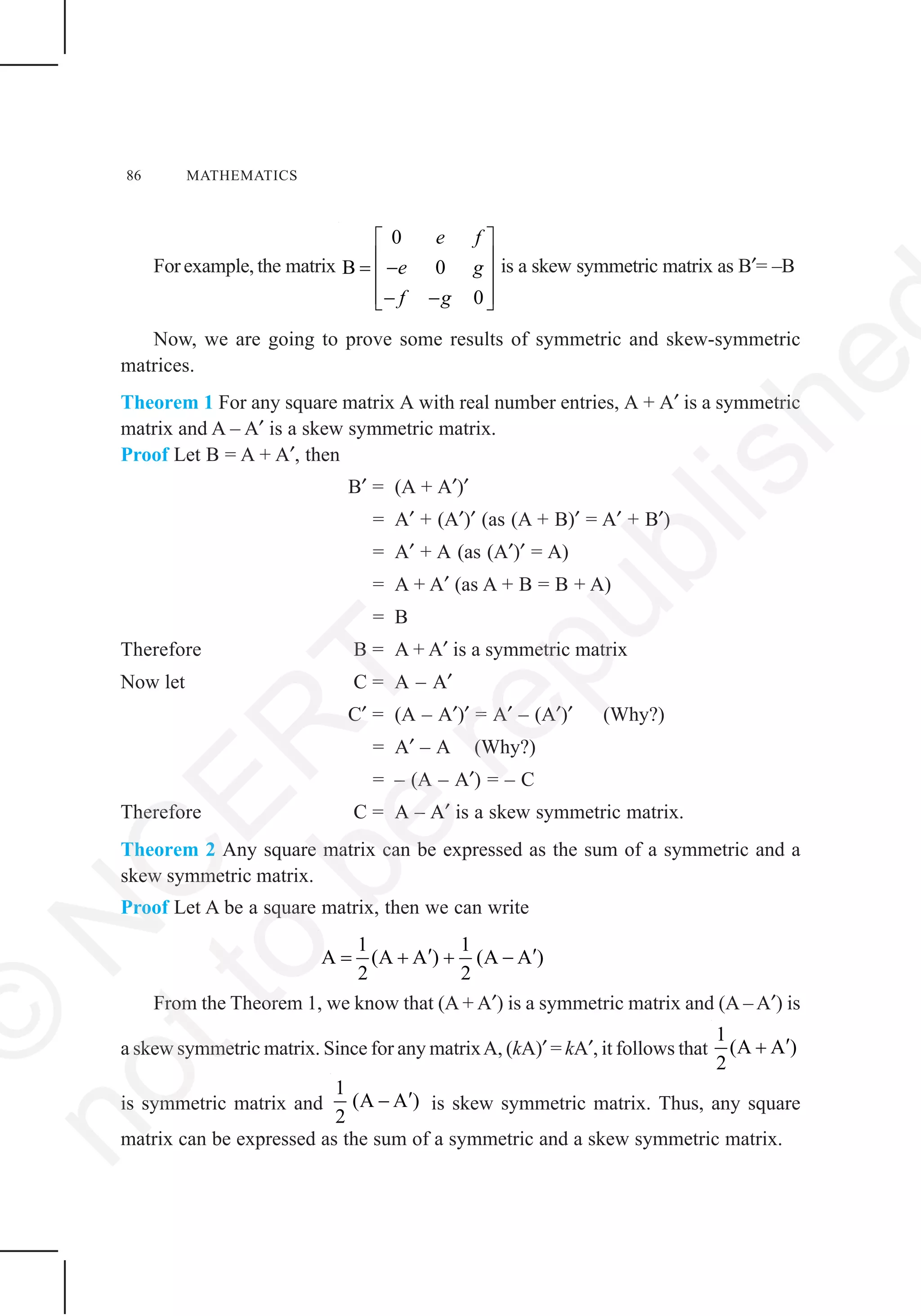
4. If A and B are symmetric matrices, prove that AB – BA is a skew symmetric
matrix.
5. Show that the matrix B′AB is symmetric or skew symmetric according as A is
symmetric or skew symmetric.
6. Find the values of x, y, z if the matrix
0 2
A
y z
x y z
x y z
⎡ ⎤
⎢ ⎥= −⎢ ⎥
⎢ ⎥−⎣ ⎦
satisfy the equation
A′A = I.
7. For what values of x : [ ]
1 2 0 0
1 2 1 2 0 1 2
1 0 2 x
⎡ ⎤ ⎡ ⎤
⎢ ⎥ ⎢ ⎥
⎢ ⎥ ⎢ ⎥
⎢ ⎥ ⎢ ⎥⎣ ⎦ ⎣ ⎦
= O?
8. If
3 1
A
1 2
⎡ ⎤
= ⎢ ⎥−⎣ ⎦
, show that A2
– 5A + 7I = 0.
9. Find x, if [ ]
1 0 2
5 1 0 2 1 4 O
2 0 3 1
x
x
⎡ ⎤ ⎡ ⎤
⎢ ⎥ ⎢ ⎥− − =⎢ ⎥ ⎢ ⎥
⎢ ⎥ ⎢ ⎥⎣ ⎦ ⎣ ⎦
©
N
C
ER
T
notto
be
republishe

46. MATRICES 101
10. A manufacturer produces three products x, y, z which he sells in two markets.
Annual sales are indicated below:
Market Products
I 10,000 2,000 18,000
II 6,000 20,000 8,000
(a) If unit sale prices of x, y and z are Rs 2.50, Rs 1.50 and Rs 1.00, respectively,
find the total revenue in each market with the help of matrix algebra.
(b) If the unit costs of the above three commodities are Rs 2.00, Rs 1.00 and 50
paise respectively. Find the gross profit.
11. Find the matrix X so that
1 2 3 7 8 9
X
4 5 6 2 4 6
− − −⎡ ⎤ ⎡ ⎤
=⎢ ⎥ ⎢ ⎥
⎣ ⎦ ⎣ ⎦
12. If A and B are square matrices of the same order such that AB = BA, then prove
by induction that ABn
= Bn
A. Further, prove that (AB)n
= An
Bn
for all n ∈ N.
Choose the correct answer in the following questions:
13. If A = is such that A² = I, then
(A) 1 + α² + βγ = 0 (B) 1 – α² + βγ = 0
(C) 1 – α² – βγ = 0 (D) 1 + α² – βγ = 0
14. If the matrix A is both symmetric and skew symmetric, then
(A) A is a diagonal matrix (B) A is a zero matrix
(C) A is a square matrix (D) None of these
15. If A is square matrix such that A2
= A, then (I + A)³ – 7 A is equal to
(A) A (B) I – A (C) I (D) 3A
Summary
A matrix is an ordered rectangular array of numbers or functions.
A matrix having m rows and n columns is called a matrix of order m × n.
[aij
]m × 1
is a column matrix.
[aij
]1 × n
is a row matrix.
An m × n matrix is a square matrix if m = n.
A = [aij
]m × m
is a diagonal matrix if aij
= 0, when i ≠ j.
©
N
C
ER
T
notto
be
republishe

47. 102 MATHEMATICS
A = [aij
]n × n
is a scalar matrix if aij
= 0, when i ≠ j, aij
= k, (k is some
constant), when i = j.
A = [aij
]n × n
is an identity matrix, if aij
= 1, when i = j, aij
= 0, when i ≠ j.
A zero matrix has all its elements as zero.
A = [aij
] = [bij
] = B if (i) A and B are of same order, (ii) aij
= bij
for all
possible values of i and j.
kA = k[aij
]m × n
= [k(aij
)]m × n
– A = (–1)A
A – B = A + (–1) B
A + B = B + A
(A + B) + C = A + (B + C), where A, B and C are of same order.
k(A + B) = kA + kB, where A and B are of same order, k is constant.
(k + l) A = kA + lA, where k and l are constant.
If A = [aij
]m × n
and B = [bjk
]n × p
, then AB = C = [cik
]m × p
, where
1
n
ik ij jk
j
c a b
=
= ∑
(i) A(BC) = (AB)C, (ii) A(B + C) = AB + AC, (iii) (A + B)C = AC + BC
If A = [aij
]m × n
, then A′ or AT
= [aji
]n × m
(i) (A′)′ = A, (ii) (kA)′ = kA′, (iii) (A + B)′ = A′ + B′, (iv) (AB)′ = B′A′
A is a symmetric matrix if A′ = A.
A is a skew symmetric matrix if A′ = –A.
Any square matrix can be represented as the sum of a symmetric and a
skew symmetric matrix.
Elementary operations of a matrix are as follows:
(i) Ri
↔ Rj
or Ci
↔ Cj
(ii) Ri
→ kRi
or Ci
→ kCi
(iii) Ri
→ Ri
+ kRj
or Ci
→ Ci
+ kCj
If A and B are two square matrices such that AB = BA = I, then B is the
inverse matrix of A and is denoted by A–1
and A is the inverse of B.
Inverse of a square matrix, if it exists, is unique.
— —
©
N
C
ER
T
notto
be
republishe