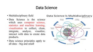
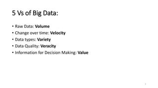
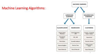
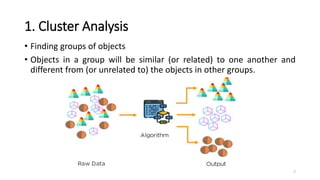
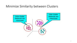
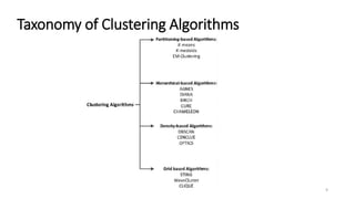
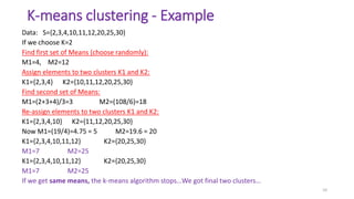
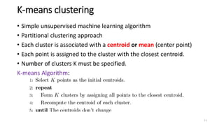
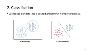
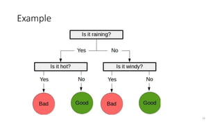
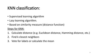
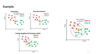
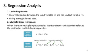
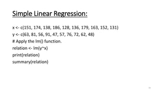
This document discusses machine learning algorithms in R. It provides an overview of machine learning, data science, and the 5 V's of big data. It then discusses two main machine learning algorithms - clustering and classification. For clustering, it covers k-means clustering, providing examples of how to implement k-means clustering in R. For classification, it discusses decision trees, K-nearest neighbors (KNN), and provides an example of KNN classification in R. It also provides a brief overview of regression analysis, including examples of simple and multiple linear regression in R.

1. Machine Learning in R
Suja A. Alex,
Assistant Professor,
Dept. of Information Technology,
St.Xavier’s Catholic College of Engineering

2. Data Science
• Multidisciplinary field
• Data Science is the science
which uses computer science,
statistics and machine learning,
visualization to collect, clean,
integrate, analyze, visualize,
interact with data to create data
products.
• Data science principles apply to
all data – big and small
2

3. 5 Vs of Big Data:
• Raw Data: Volume
• Change over time: Velocity
• Data types: Variety
• Data Quality: Veracity
• Information for Decision Making: Value
3

4. Machine Learning Algorithms:
4

5. Input: Datasets in R
• https://vincentarelbundock.github.io/Rdatasets/datasets.html
• http://archive.ics.uci.edu/ml/datasets.php
• https://www.kaggle.com/datasets
5

6. Output: Data Visualization Packages in R
• graphics - plot(), barplot(), boxplot()
• ggplot2 - Scatterplot
• lattice - tiled plots
• plotly - Line plot, Time series chart, interactive 3D plots
6

7. 1. Cluster Analysis
• Finding groups of objects
• Objects in a group will be similar (or related) to one another and
different from (or unrelated to) the objects in other groups.
7

8. Minimize Similarity between Clusters
8

9. Taxonomy of Clustering Algorithms
9

10. K-means clustering - Example
Data: S={2,3,4,10,11,12,20,25,30}
If we choose K=2
Find first set of Means (choose randomly):
M1=4, M2=12
Assign elements to two clusters K1 and K2:
K1={2,3,4} K2={10,11,12,20,25,30}
Find second set of Means:
M1=(2+3+4)/3=3 M2=(108/6)=18
Re-assign elements to two clusters K1 and K2:
K1={2,3,4,10} K2={11,12,20,25,30}
Now M1=(19/4)=4.75 = 5 M2=19.6 = 20
K1={2,3,4,10,11,12} K2={20,25,30}
M1=7 M2=25
K1={2,3,4,10,11,12} K2={20,25,30}
M1=7 M2=25
If we get same means, the k-means algorithm stops…We got final two clusters…
10

11. K-means clustering
• Simple unsupervised machine learning algorithm
• Partitional clustering approach
• Each cluster is associated with a centroid or mean (center point)
• Each point is assigned to the cluster with the closest centroid.
• Number of clusters K must be specified.
K-means Algorithm:
11

12. Clustering packages in R
1. Cluster
2. ClusterR
3. NbClust
Function for k-means in R:
kmeans(x, centers, nstart)
where x  numeric dataset (matrix or data frame)
centers  number of clusters to extract
nstart  generate number of initial configurations
12

13. K-means-clustering in R
// Before Clustering
// Explore data
library(datasets)
head(iris)
library(ggplot2)
ggplot(iris, aes(Petal.Length, Petal.Width, color = Species)) + geom_point()
// After K-means Clustering
set.seed(20)
irisCluster <- kmeans(iris[, 3:4], 3)
irisCluster
irisCluster$cluster <- as.factor(irisCluster$cluster)
ggplot(iris, aes(Petal.Length, Petal.Width, color = irisCluster$cluster)) + geom_point()
13

14. 2. Classification
• Categorize our data into a desired and distinct number of classes.
14

15. Example:
15

16. Classification Algorithm
• Decision Tree
• Bayes Classifier
• Nearest Neighbor
• Support Vector Machines
• Naive Linear Classifiers (or Logistic Regression)
16

17. 1. Decision Tree
17

18. Example Decision Tree:
18

19. Example
19

20. KNN classification:
• Supervised learning algorithm
• Lazy learning algorithm.
• Based on similarity measure (distance function)
Steps for KNN:
1. Calculate distance (e.g. Euclidean distance, Hamming distance, etc.)
2. Find k closest neighbors
3. Vote for labels or calculate the mean
20

21. Example:
21

22. KNN classification in R
df <- data(iris) ##load data
head(iris) ## see the stucture
##Generate a random number that is 90% of the total number of rows in dataset.
ran <- sample(1:nrow(iris), 0.9 * nrow(iris))
##the normalization function is created
nor <-function(x) { (x -min(x))/(max(x)-min(x)) }
##Run nomalization on first 4 coulumns of dataset because they are the predictors
iris_norm <- as.data.frame(lapply(iris[,c(1,2,3,4)], nor))
summary(iris_norm)
##extract training set
iris_train <- iris_norm[ran,]
##extract testing set
iris_test <- iris_norm[-ran,]
##extract 5th column of train dataset because it will be used as 'cl' argument in knn function.
iris_target_category <- iris[ran,5]
##extract 5th column if test dataset to measure the accuracy
iris_test_category <- iris[-ran,5]
##load the package class
library(class)
##run knn function
pr <- knn(iris_train,iris_test,cl=iris_target_category,k=13)
##create confusion matrix
tab <- table(pr,iris_test_category)
##this function divides the correct predictions by total number of predictions that tell us how accurate teh
model is.
accuracy <- function(x){sum(diag(x)/(sum(rowSums(x)))) * 100}
accuracy(tab)
22

23. 3. Regression Analysis
1. Linear Regression:
• linear relationship between the input variable (x) and the soutput variable (y).
• Fitting a straight line to data.
2. Multiple linear regression:
When there are multiple input variables, literature from statistics often refers to
the method as multiple linear regression.
23

24. Simple Linear Regression:
x <- c(151, 174, 138, 186, 128, 136, 179, 163, 152, 131)
y <- c(63, 81, 56, 91, 47, 57, 76, 72, 62, 48)
# Apply the lm() function.
relation <- lm(y~x)
print(relation)
summary(relation)
24

25. Multiple Linear Regression:
input <- mtcars[,c("mpg","disp","hp","wt")]
print(head(input))
// Create Relationship Model & get the Coefficients
input <- mtcars[,c("mpg","disp","hp","wt")]
# Create the relationship model.
model <- lm(mpg~disp+hp+wt, data = input)
# Show the model.
print(model)
# Get the Intercept and coefficients as vector elements.
cat("# # # # The Coefficient Values # # # ","n")
a <- coef(model)[1]
print(a)
Xdisp <- coef(model)[2]
Xhp <- coef(model)[3]
Xwt <- coef(model)[4]
print(Xdisp)
print(Xhp)
print(Xwt)
25