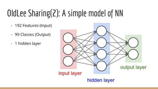
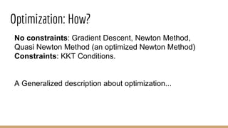
Downloaded 45 times
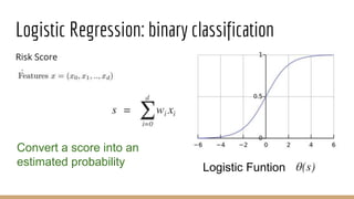
![Logistic Regression : Motivation
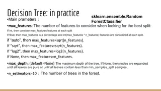
Targrt Function: f(x) = P(+1|x) is with in [0,1]](https://image.slidesharecdn.com/mlrecall-161221144430/85/Machine-Learning-Algorithms-Part-1-12-320.jpg)
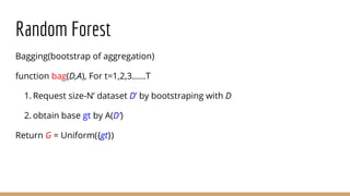
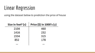
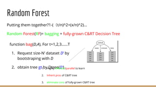
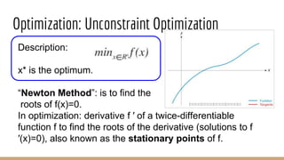
![Random Forest
Decision Tree
funcion Tree(D)
if ternimation return base gt else
1. learn b(x) then split D to Dc by b(x)
2. build Gc <- Tree(Dc)
3. return G(x)=∑[bx=c]Gc(x)
Bagging: reduce variance by voting/averaging
Decision Tree: large variance especially in fully-grown tree](https://image.slidesharecdn.com/mlrecall-161221144430/85/Machine-Learning-Algorithms-Part-1-21-320.jpg)
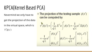
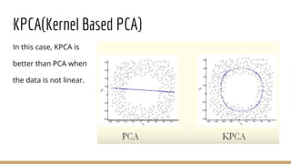
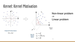
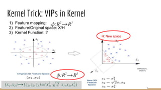
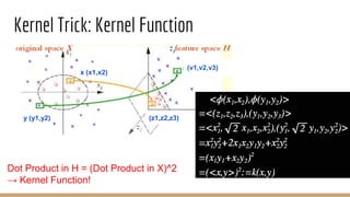
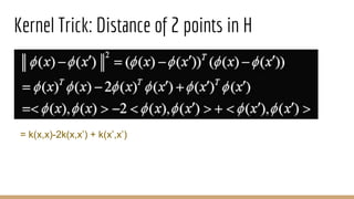
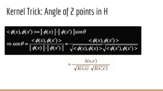
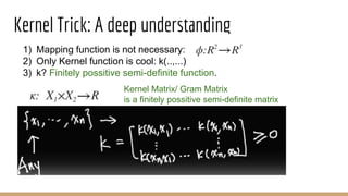
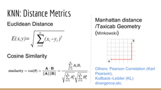

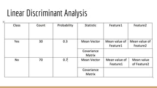
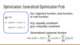
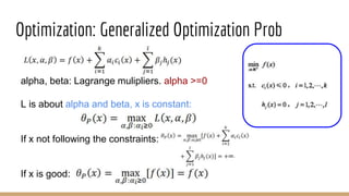
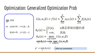
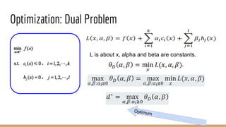
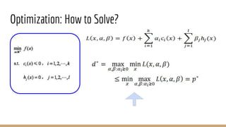
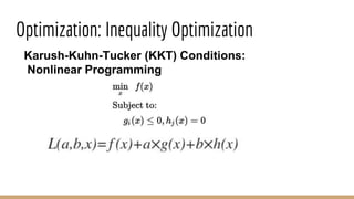


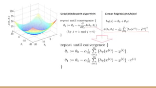
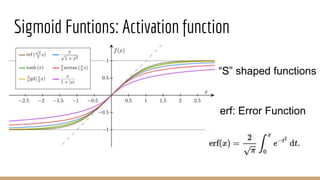
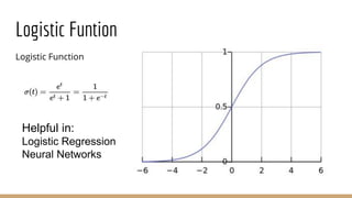
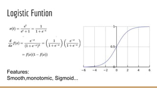
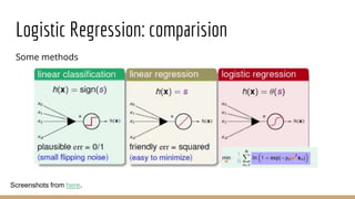
This document provides an overview of various machine learning algorithms and concepts, including supervised learning techniques like linear regression, logistic regression, decision trees, random forests, and support vector machines. It also discusses unsupervised learning methods like principal component analysis and kernel-based PCA. Key aspects of linear regression, logistic regression, and random forests are summarized, such as cost functions, gradient descent, sigmoid functions, and bagging. Kernel methods are also introduced, explaining how the kernel trick can allow solving non-linear problems by mapping data to a higher-dimensional feature space.