Download as PDF, PPTX


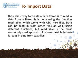
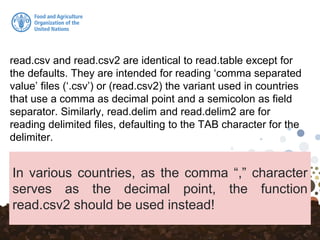


![R- Import Data
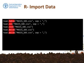
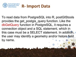
> is.na(SOC)
Id UpperDepth LowerDepth SOC Lambda tsme Region
[1,] FALSE FALSE FALSE FALSE FALSE FALSE FALSE
[2,] FALSE FALSE FALSE FALSE FALSE FALSE FALSE
[3,] FALSE FALSE FALSE FALSE FALSE FALSE FALSE
[4,] FALSE FALSE FALSE FALSE FALSE FALSE FALSE
[5,] FALSE FALSE FALSE FALSE FALSE FALSE FALSE
[6,] FALSE FALSE FALSE FALSE FALSE FALSE FALSE
[7,] FALSE FALSE FALSE FALSE FALSE FALSE FALSE
[8,] FALSE FALSE FALSE FALSE FALSE FALSE FALSE
[9,] FALSE FALSE FALSE FALSE FALSE FALSE FALSE
[10,] FALSE FALSE FALSE FALSE FALSE FALSE FALSE
...](https://image.slidesharecdn.com/ir-d23-rdata-import-data-export-180321133113/85/R-data-import-data-export-8-320.jpg)
![R- Import Data
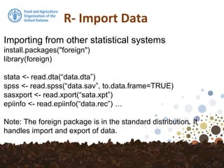
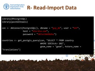
> anyNA(SOC)
[1] TRUE
> sum(is.na(SOC$SOC))
[1] 1](https://image.slidesharecdn.com/ir-d23-rdata-import-data-export-180321133113/85/R-data-import-data-export-9-320.jpg)


The document provides an overview of various methods for importing and exporting data in R, particularly focusing on reading data from files, web sources, and spatial databases like PostGIS. It covers specific functions such as read.table, read.csv, and the use of the foreign package to handle different data formats. Additionally, it discusses saving data in R's own format and the importance of preserving data attributes.