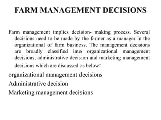
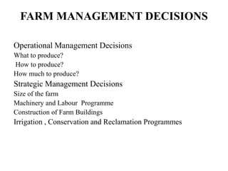
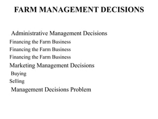
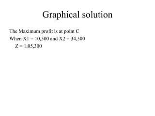
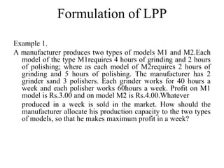
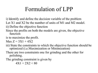
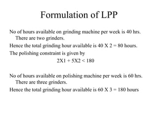
The document provides an overview of a presentation on decision making and linear programming. It discusses farm management decisions that fall under organizational, administrative, and marketing categories. It then introduces quantitative analysis approaches and linear programming. Linear programming is defined as a technique to optimize performance under resource constraints. The assumptions and terminology of linear programming are explained. Finally, examples are provided to demonstrate how to formulate a linear programming model and solve it graphically.

1. AN
PRESENTATION
ON
“DECISION MAKING, INTRODUCTION TO LINEAR
PROGRAMMING AND GRAPHICAL SOLUTION”
GUIDED BY,
DR. H. PATHAK PRESENTED BY,
ASSTT.PROFESSOR DWARIKADHISH CHURPAL
DEPT.OF AGRIL.ECONOMICS M.Sc (Ag.) PREVIOUS
COA, RAIPUR AGRIL. ECONOMICS
College of agriculture Raipur
Indira Gandhi Agricultural University, Raipur

2. FARM MANAGEMENT DECISIONS
Farm management implies decision- making process. Several
decisions need to be made by the farmer as a manager in the
organizational of farm business. The management decisions
are broadly classified into organizational management
decisions, administrative decision and marketing management
decisions which are discussed as below:
organizational management decisions
Administrative decision
Marketing management decisions

3. FARM MANAGEMENT DECISIONS
Operational Management Decisions
What to produce?
How to produce?
How much to produce?
Strategic Management Decisions
Size of the farm
Machinery and Labour Programme
Construction of Farm Buildings
Irrigation , Conservation and Reclamation Programmes

4. FARM MANAGEMENT DECISIONS
Administrative Management Decisions
Financing the Farm Business
Financing the Farm Business
Financing the Farm Business
Marketing Management Decisions
Buying
Selling
Management Decisions Problem

5. Introduction to Quantitative analysis
Small size of holdings
Inadequate capital
Lack of Labour
Lack of technology
Marking problem
Quantitative analysis
Introduction :
Quantitative Analysis a scientific approach to managerial
decision making where by raw data are processed and
manipulation resulting in managerial information.

6. Introduction to Quantitative analysis
• Quantitative analysis Approaches
• Defining the problem
• Developing a Models
• Aeqising inputed
• Developing a solution
• Testing the solution
• Analyzing the result
• Implementing the result

7. Introduction to Linear Programming
Linear Programming
Introduction
• Linear programming was developed during World
War II, when a system with which to maximize the e_ciency of
resources was of utmost importance.
• New War-related projects demanded attention and spread
resources thin. Programming"
• Was a military term that referred to activities such as planning
schedules?

8. Introduction to Linear Programming
Definition:
Linear programming is a mathematical
technique to optimize performance (eg profit or cost)
under a set resources constraints (eg machine hours,
man hours, money material etc.) as specified by an
organization.

9. Introduction to Linear Programming
Concept
Decision variable
Objective function coefficient
Technological coefficient
Availability of resources

10. Introduction to Linear Programming
Assumptions
Certainty
Linearity
Proportionality
Additivity
Multiplictivity
Divisibility (Continuity)
Non negative Constance

11. Introduction to Linear Programming
• General Mathematical Model of an LPP
• Optimize (Maximize or Minimize) Z=C1 X1 + C2 X2
+……+CnXn
• Subject to constraints,
• a11X1+ a 12X2+………………+ a 1nXn (<,=,>) b1
• a21X1+ a 22X2+………………+ a 2nXn (<,=,>) b2
• a31X1+ a 32X2+………………+ a 3nXn (<,=,>) b3
• am1X1+ a m2X2+………………+ a mnXn (<,=,>)
bm
• and X1, X2 ….Xn >

12. Introduction to Linear Programming
Guidelines for formulating Linear Programming model
i) Identify and define the decision variable of the problem
ii) Define the objective function
iii) State the constraints to which the objective function should be
optimized (i.e. Maximization or Minimization)
iv) Add the non-negative constraints from the consideration that
the negative values of the decision variables do not
have any valid physical interpretation

13. Introduction to Linear Programming
Terminology:
The function to be maximized or minimized is called the
objective function.
A vector, x for the standard maximum problem or y for the
standard minimum problem, is said to be feasible if it satisfies
the corresponding constraints.
The set of feasible vectors is called the constraint set.
A linear programming problem is said to be feasible if the
constraint set is not empty; otherwise it is said to be infeasible.

14. Introduction to Linear Programming
• A feasible maximum (resp. minimum) problem is said to
be unbounded if the objective function can assume
arbitrarily large positive (resp. negative) values at feasible
vectors; otherwise, it is said to be bounded. Thus there
are three possibilities for a linear programming problem.
It may be bounded feasible, it may be unbounded
feasible, and it may be infeasible.
• The value of a bounded feasible maximum (resp,
minimum) problem is the maximum (resp. minimum)
value of the objective function as the variables range over
the constraint set.
• A feasible vector at which the objective function achieves
the value is called optimal

15. Graphical solution
Example -
Solve the following LPP by graphical method
Minimize Z = 20X1 + 40X2
Subject to constraints
36X1 + 6X2 ≥ 108
3X1 + 12X2 ≥ 36
20X1 + 10X2 ≥ 100
X1 X2 ≥ 0

16. Graphical solution
Solution:
The first constraint 36X1 + 6X2 ≥ 108 can be represented as follows.
We set 36X1 + 6X2 = 108
When X1 = 0 in the above constraint, we get
36 x 0 + 6X2 = 108
X2 = 108/6 = 18
Similarly when X2 = 0 in the above constraint, we get,
36X1 + 6 x 0 = 108
X1 = 108/36 = 3
The second constraint3X1 + 12X2 ≥ 36 can be represented as follows,
We set 3X1 + 12X2 = 36
When X1 = 0 in the above constraint, we get,
3 x 0 + 12X2 = 36
X2 = 36/12 = 3

17. Graphical solution
Similarly when X2 = 0 in the above constraint, we get,
3X1 + 12 x 0 = 36
X1 = 36/3 = 12
The third constraint20X1 + 10X2 ≥ 100 can be represented as
follows,
We set 20X1 + 10X2 = 100
When X1 = 0 in the above constraint, we get,
20 x 0 + 10X2 = 100
X2 = 100/10 = 10
Similarly when X2 = 0 in the above constraint, we get,
20X1 + 10 x 0 = 100
X1 = 100/20 = 5

18. Graphical solution

19. Graphical solution
Point X1 X2 Z = 20X1 + 40X2
0 0 0 0
A 0 18 Z = 20 x 0 + 40 x 18 = 720
B 2 6 Z = 20 x2 + 40 x 6 = 280
C 4 2 Z = 20 x 4 + 40 x 2 = 160*
Minimum
D 12 0 Z = 20 x 12 + 40 x 0 = 240
The Minimum cost is at point C
When X1 = 4 and X2 = 2
Z = 160

20. Graphical solution
Example.
Solve the following LPP by graphical method
Maximize Z = 2.80X1 + 2.20X2
Subject to constraints
X1 ≤ 20,000
X2 ≤ 40,000
0.003X1 + 0.001X2 ≤ 66
X1 + X2 ≤ 45,000
X1 X2 ≥ 0

21. Graphical solution
Solution:
The first constraint X1 ≤ 20,000 can be represented as follows.
We set X1 = 20,000
The second constraint X2 ≤ 40,000 can be represented as follows,
We set X2 = 40,000
The third constraint 0.003X1 + 0.001X2 ≤ 66 can be represented as follows,
We set 0.003X1 + 0.001X2 = 66
When X1 = 0 in the above constraint, we get,
0.003 x 0 + 0.001X2 = 66
X2 = 66/0.001 = 66,000
Similarly when X2 = 0 in the above constraint, we get,
0.003X1 + 0.001 x 0 = 66
X1 = 66/0.003 = 22,000

22. Graphical solution
The fourth constraint X1 + X2 ≤ 45,000 can be represented as
follows,
We set X1 + X2 = 45,000
When X1 = 0 in the above constraint, we get,
0 + X2 = 45,000
X2 = 45,000
Similarly when X2 = 0 in the above constraint, we get,
X1 + 0 = 45,000
X1 =45,000

23. Graphical solution

24. Point X1 X2 Z = 2.80X1 + 2.20X2
0 0 0 0
A 0 40,000 Z = 2.80 x 0 + 2.20 x 40,000 =88,000
B 5,000 40,000
Z = 2.80 x 5,000 + 2.20 x 40,000 =
1,02,000
C 10,500 34,500
1,05,300* Maximum
D 20,000 6,000
Z = 2.80 x 20,000 + 2.20 x 6,000 =69,200
E 20,000 0 Z = 2.80 x 20,000 + 2.20 x 0 = 56,000

25. Graphical solution
The Maximum profit is at point C
When X1 = 10,500 and X2 = 34,500
Z = 1,05,300

26. Formulation of LPP
Example 1.
A manufacturer produces two types of models M1 and M2.Each
model of the type M1requires 4 hours of grinding and 2 hours
of polishing; where as each model of M2requires 2 hours of
grinding and 5 hours of polishing. The manufacturer has 2
grinder sand 3 polishers. Each grinder works for 40 hours a
week and each polisher works 60hours a week. Profit on M1
model is Rs.3.00 and on model M2 is Rs.4.00.Whatever
produced in a week is sold in the market. How should the
manufacturer allocate his production capacity to the two types
of models, so that he makes maximum profit in a week?

27. Formulation of LPP
i) Identify and define the decision variable of the problem
Let X1 and X2 be the number of units of M1 and M2 model.
ii) Define the objective function
Since the profits on both the models are given, the objective
function
is to maximize the profit.
Max Z = 3X1 + 4X2
iii) State the constraints to which the objective function should be
optimized (i.e.Maximization or Minimization)
There are two constraints one for grinding and the other for
polishing.
The grinding constraint is given by
4X1 + 2X2 < 80

28. Formulation of LPP
No of hours available on grinding machine per week is 40 hrs.
There are two grinders.
Hence the total grinding hour available is 40 X 2 = 80 hours.
The polishing constraint is given by
2X1 + 5X2 < 180
No of hours available on polishing machine per week is 60 hrs.
There are three grinders.
Hence the total grinding hour available is 60 X 3 = 180 hours

29. Formulation of LPP
Finally we have,
Max Z = 3X1 + 4X2
Subject to constraints,
4X1 + 2X2 < 80
2X1 + 5X2 < 180
X1, X2 > 0

30. Formulation of LPP
Example 2.
A firm is engaged in producing two products. A and B. Each
unit of product A requires 2kg of raw material and 4
labour hours for processing, where as each unit of B
requires 3kg of raw materials and 3 labour hours for the
same type. Every week, the firm has an availability of 60
kg of raw material and 96 labour hours. One unit of
product A sold yields Rs.40 and one unit of product B
sold gives Rs.35 as profit.
Formulate this as an Linear Programming Problem to
determine as to how many units of each of the products
should be produced per week so that the firm can earn
maximum profit.

31. Formulation of LPP
i) Identify and define the decision variable of the problem
Let X1 and X2 be the number of units of product A and product B
produced per week.
ii) Define the objective function
Since the profits of both the products are given,
the objective function is to maximize the profit.
MaxZ = 40X1 + 35X2
iii) State the constraints to which the objective function should be
optimized (i.e.Maximization or Minimization)

32. Formulation of LPP
There are two constraints one is raw material constraint and the other
one is labourconstraint..
The raw material constraint is given by
2X1 + 3X2 < 60
The labour hours constraint is given by
4X1 + 3X2 < 96
Finally we have,
Max Z = 40X1 + 35X2
Subject to constraints,
2X1 + 3X2 < 60
4X1 + 3X2 < 96
X1, X2 > 0

33. Thanks