The document introduces linear programming and provides examples to illustrate its basic concepts and formulation. It defines linear programming as a technique to optimally allocate limited resources according to a given objective function and set of linear constraints. It then provides definitions for key linear programming components - decision variables, objective function, and constraints. Examples are provided to demonstrate how to formulate linear programming problems from descriptions of resource allocation scenarios and how to represent them mathematically.
![Linear Programming 15
ai1 x1 + ai2 x2 + ai3 x3 + … + ain xn (£, =, ≥) bi
am1 x1 + am2 x2 + am3 x3 + … + amn xn (£, =, ≥) bm
and x1, x2, x3… xn ≥ 0 (3)
Equation (1) is known as objective function.
Equation (2) represents the role of constants.
Equation (3) is non-negative restrictions.
Also aij
¢s bj¢s and cj¢s are constants and xj¢s are decision variables.
The above L.P.P. can be expressed in the form of matrix as follows:
Opt. Z = CX,
Subject to
AX (£, =, ≥) B
and X ≥ 0
where C = c1, c2, c3 … cn
X = x1, x2, x3 … xn
B =
b
b
bm
1
2
È
Î
Í
Í
Í
Í
˘
˚
˙
˙
˙
˙
A =
a a
a a a
a a a
n
n
m m mn m n
11 12 1
21 22 2
1 2
a º
º
º
È
Î
Í
Í
Í
Í
˘
˚
˙
˙
˙
˙
¥
= [aij]m¥n
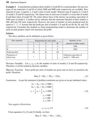
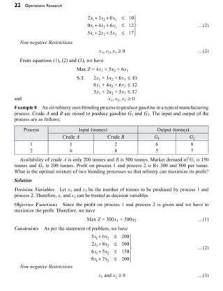
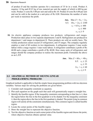
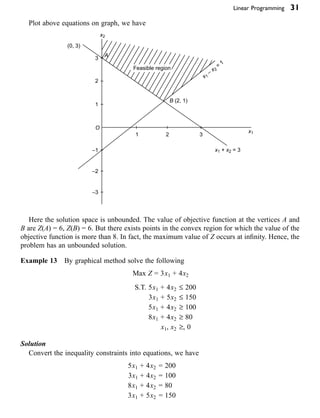
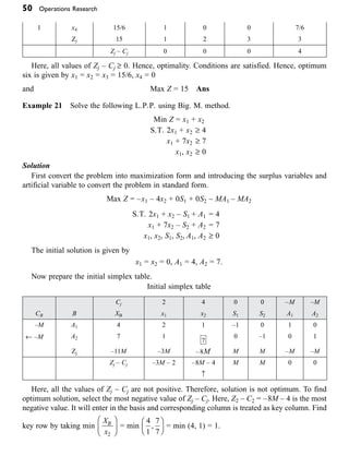
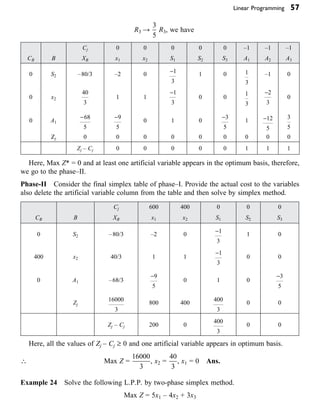
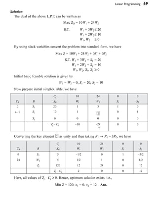
Example 1 A manufacturer produces two types of models M1 & M2. Each model of type M1
requires 4 hr of grinding and 2 hr of polishing. Whereas model M2 requires 2 hr of grinding and
5 hr of polishing. The manufacturer has 2 grinders and 3 polishers. Each grinder works 60 hr a
week and each polisher works 50 hr a week. Profit on model M1 is Rs 4.00 and on model M2 is Rs
5.00. How should the manufacturer allocate his production capacity to the two types of models, so
that he may make the maximum profit in a weak? Formulate it as linear programming problem.
Solution
Decision Variables Let x1 and x2 be the number of units produced model M1 and model M2.
Therefore, x1 and x2 be treated as decision variables.
Objective Function Since the profit on both the models is given and we have to maximize the
profit. Therefore,
Max Z = 4x1 + 5x2 …(1)](https://image.slidesharecdn.com/181sample-chapter-221017205802-782c7ea6/85/181_Sample-Chapter-pdf-2-320.jpg)
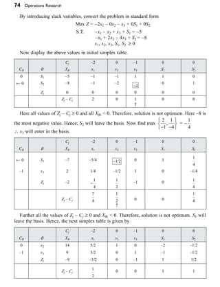
![34 Operations Research
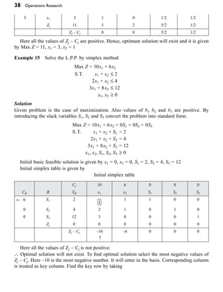
6. Max Z = 3x1 – 2x2
S.T. x1 + x2 £ 1
2x1 + 2x2 ≥ 6
3x1 + 2x2 ≥ 48
x1, x2 ≥ 0
[Ans. No feasible solution]
7. Min Z = 3x1 – 2x2
S.T. x1 + x2 £ 1
2x1 + 2x2 ≥ 6
3x1 + 2x2 ≥ 48
x1, x2 ≥ 0
[Ans. No feasible solution]
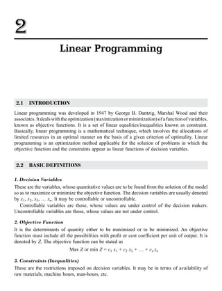
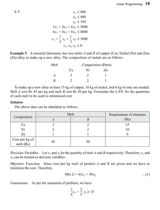
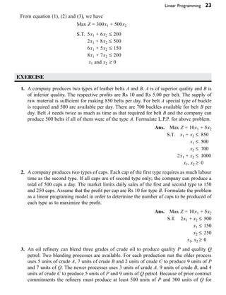
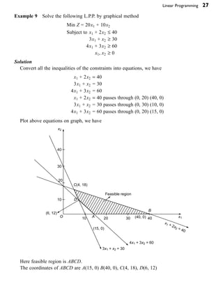
8. A company produces two different products A and B. The company makes a profit of Rs
40 and Rs 30 per unit on A and B respectively. The production process has a capacity of
30,000 man hours. It takes 3 hr to produce one unit of a A and one hr to produce one unit
of B. The market survey indicates that the maximum number of units of product A that
can be sold is 8000 and those of B is 12,000 units. Formulate the problem and solve it by
graphical method to get maximum profit.
Ans. Max Z = 40x1 + 30x2
S.T. 3x1 + x2 £ 30,000
x1 £ 8000
x2 £ 12000
x1, x2 ≥ 0
[Ans. x1 = 6000, x2 = 1200, Max Z = 600000]
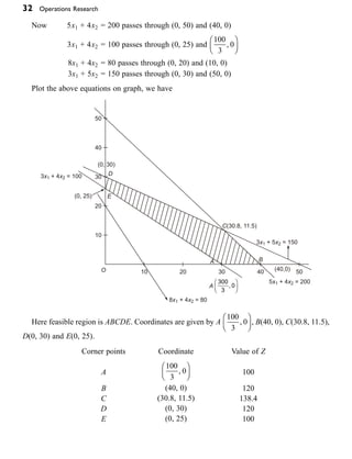
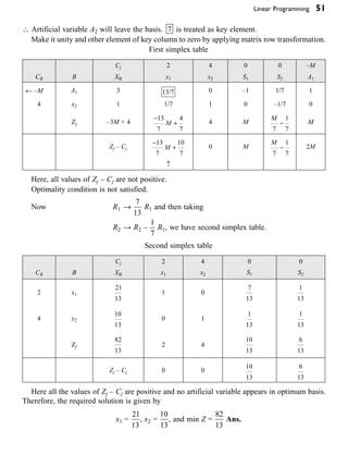
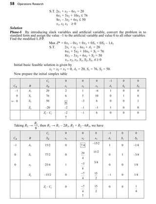
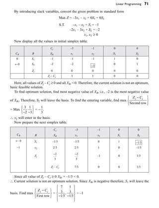
2.6 SIMPLEX METHOD
It is an iterative procedure for solving an L.P.P. in a finite number of steps. This method provides
an algorithm which consists of moving from one vertex of the region of feasible solution to
another in such a manner that the value of the objective function at the successing vertex is less
or more as the case may be more than its process vertex. This procedure is repeated and since
the number of vertices is finite, the method leads to an optimal vertex in a finite number of steps
or indicates the existence of unbounded solutions. It is applicable for any number of decision
variables.
2.6.1 Basic Terms Involved in Simplex Method
1. Standard Form of an L·P·P
. In standard form of the objective function, namely, maximize
or minimize, all the constraints are expressed as equations moreover R.H.S. of each constraint
and all variables are non-negative.
2. Slack Variables These variables are added to less than or equal to type constraints to change
it into equality.](https://image.slidesharecdn.com/181sample-chapter-221017205802-782c7ea6/85/181_Sample-Chapter-pdf-18-320.jpg)
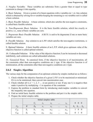
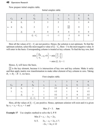
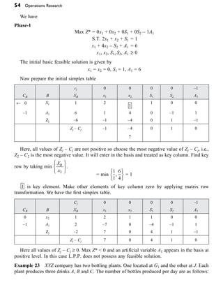
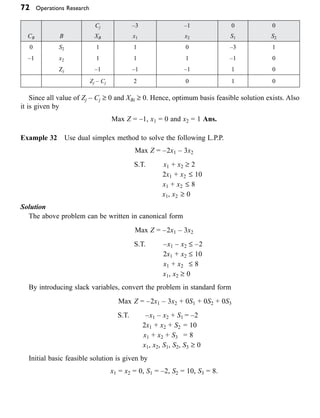
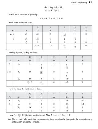
![44 Operations Research
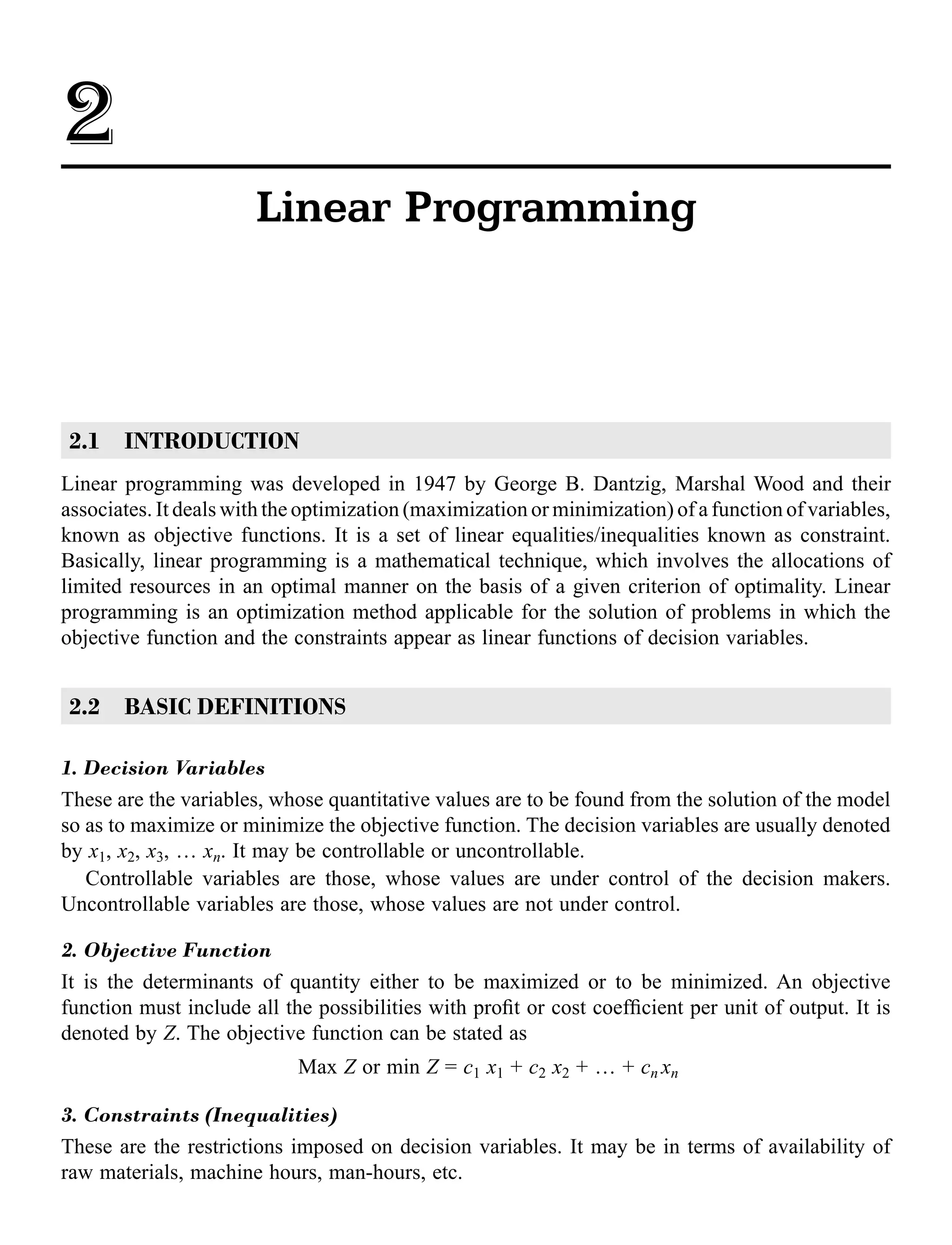
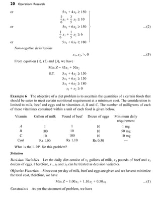
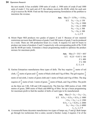
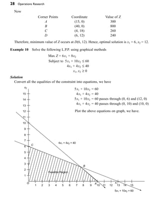
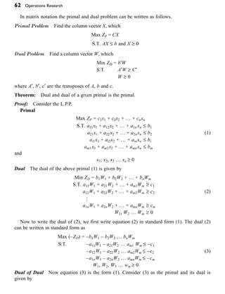
First simplex table
Cj 3 2 5 0 0 0
CB B XB x1 x2 x3 S1 S2 S3
0 S1 200
-1
2
2 0 1 1/2 0
5 x3 230
3
2
0 1 0 1/2 0
0 S3 420 1 4 0 0 0 1
Zj 1150 15/2 0 5 0 5/2 0
Zj – Cj
9
2
–2 0 0 5/2 0
≠
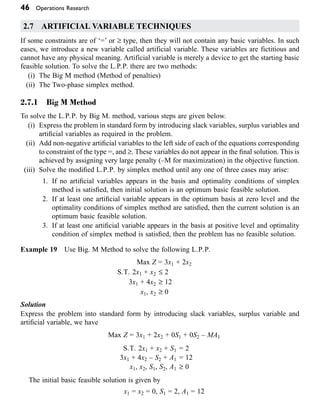
Further, all values of Zj – Cj are not positive. Hence, repeat the above process.
2 is the key element. Make it unity and other elements of key column zero by applying matrix
row transformation, we have the second simplex table.
Second simplex table
Cj 3 2 5 0 0 0
CB B XB x1 x2 x3 S1 S2 S3
2 x2 100 –1/4 1 0 1/2 –1/4 0
5 x3 230 3/2 0 1 0 1/2 0
0 s3 20 2 0 0 –2 1 1
Zj 1350 7 2 5 1 2 0
Zj – Cj 4 0 0 1 2 0
Since all values of Zj – Cj ≥ 0. Hence, the solution is optimum. It is given by
x1 = 0, x2 = 100, x3 = 230, Max Z = 1350 Ans
EXERCISE
Solve the Following L.P.P. by simplex method.
1. Max Z = x1 + 2x2 + x3
S.T. 2x1 + x2 – x3 ≥ –2
–2x1 + x2 –5x3 £ 6
4x1 + x2 + x3 £ 6
x1, x2, x3 ≥ 0
[Ans. x1 = 0, x2 = 4, x3 = 2 Max Z = 10]](https://image.slidesharecdn.com/181sample-chapter-221017205802-782c7ea6/85/181_Sample-Chapter-pdf-25-320.jpg)
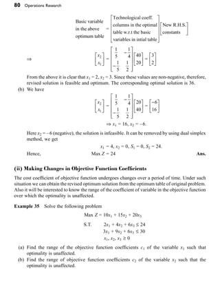
![Linear Programming 53
7. Min Z = 12x1 + 20x2.
S.T. 6x1 + 8x2 ≥ 100
7x1 + 12x2 ≥ 120
x1, x2 ≥ 0
[Ans. Min Z = 205, x1 = 15, x2 =
5
4
]
8. Min Z = 5x + 3y
S.T. 2x + 4y £ 12
2x + 2y = 10
5x + 2y ≥ 10
x, y ≥ 0
[Ans. x = 4, y = 1, Min Z = 23]
2.7.2 Two-phase Simplex Method
This method is another method to solve a given L.P.P. involving some artificial variable. In this
method solution is obtained in two phases.
Phase-I In this phase, we construct an auxiliary L.P.P. leading to a final simplex table. Various
steps are given below:
(i) Assign cost – 1 to each artificial variable and cost 0 to all other variables. Also find a new
objective function Z*.
(ii) Solve the auxiliary L.P.P by simplex method until either following three cases arise.
(i) Max Z* < 0 and at least one artificial variable appears in the optimum basis at positive
level. In this case L.P.P. dose not possess any feasible solution.
(ii) Max Z* = 0 and at least one artificial variable or no artificial variable appears in
optimum basis. In both the cases, we go to the phase II.
Phase-II Use solution of phase 1 as the initial value of phase-II. Assign the actual cost to the
variables and zero cost of every artificial variable. Delete the artificial variable column from the
table. Apply simplex method to the modified simplex table to find the solution.
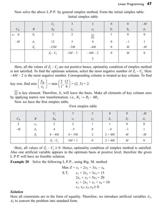
Example 22 Use two-phase simplex method to solve
Max Z = 5x1 + 3x2
S.T. 2x1 + x2 £ 1
x1 + 4x2 ≥ 6
x1, x2 ≥ 0
Solution
We convert the given problem in standard form by introducing slack variable, surplus variable
and artificial variable. Also assign the cost – 1 to artificial variable and the cost 0 to another
variables.](https://image.slidesharecdn.com/181sample-chapter-221017205802-782c7ea6/85/181_Sample-Chapter-pdf-32-320.jpg)
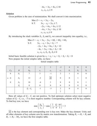
![60 Operations Research
6x1 + x2 + 6x3 ≥ 12
x1, x2, x3 ≥ 0
[Ans. Max Z = –15, x1 =
3
2
, x2 = 3, x3 = 0]
2. Min Z = 12x1 + 18x2 + 15x3
S.T. 4x1 + 8x2 + 6x3 ≥ 64
3x1 + 6x2 + 12x3 ≥ 96
x1, x2, x3 ≥ 0
[Ans. x1 = 0, x2 =
16
5
, x3 =
32
5
, Min Z =
768
5
]
3. Min Z = 10x1 + 6x2 + 2x3
S.T. –x1 + x2 + x3 ≥ 1
3x1 + x2 – x3 ≥ 2
x1, x2, x3 ≥ 0
[Ans. x1 =
1
4
, x2 =
5
4
, Min Z = 10 x3 = 0]
4. Min Z = –2x1 – x2
S.T. x1 + x2 ≥ 2
x1 + x2 £ 4
x1, x2 ≥ 0
[Ans. Min Z = –8, x1 = 4, x2 = 0]
5. Max Z = 2x1 + x2 + x3
S.T. 4x1 + 6x2 + 3x3 £ 8
3x1 – 6x2 – 4x3 £ 1
2x1 + 3x2 – 5x3 ≥ 4
x1, x2, x3 ≥ 0
[Ans. x1 =
9
7
, x2 =
10
21
, x3 = 0, Max Z =
64
21
]
6. Max Z = 5x1 + 3x2
S.T. x1 + x2 = 5
x1 + 2x2 £ 6
5x1 + 2x2 ≥ 10
x1, x2 ≥ 0
[Ans. Min Z = 23, x1 = 4, x2 = 1]
7. Max Z = x1 + x2
S.T. x1 + x2 ≥ 2
x1 + 3x2 £ 3
x1, x2 ≥ 0
[Ans. Max Z = 3, x1 = 3, x2 = 0]](https://image.slidesharecdn.com/181sample-chapter-221017205802-782c7ea6/85/181_Sample-Chapter-pdf-37-320.jpg)
![Linear Programming 63
Min ZD = –c1v1 – c2v2 … cnvn
S.T. –a11v1 – a12v2 … a1nvn ≥ –b1
–a21v1 – a22v2 … –a2nvm ≥ –b2
…
–am1v1 – am2v2 … amnvn≥ bm
v1, v2 … vm ≥ 0 (4)
The above dual can also be written as
Max ZD = c1v1 + c2v2 + … + cnvn
S.T. a11v1 + a12v2 + … + a1nvn £ b1
a21v1 + a22v2 + … + a2nvn £ b2
…
am1v1 + am2v2 + … + amn Vn £ bm
v1, v2, v3 … vn ≥ 0 (5)
Equation (5) is identical to (1). Hence, it is proved that dual and dual of a given primal is
the primal.
Example 25 Write the dual of the problem
Min Z = 3x1 + x2
S.T. 2x1 + 3x2 ≥ 2
x1 + x2 ≥ 1
x1, x2 ≥ 0
Solution
The given L.P.P. is in the standard primal form. In matrix notation it is written as
Min ZP = (3, 1) [x1, x2] = CX
S.T.
2 3
1 1
1
2
È
Î
Í
˘
˚
˙
È
Î
Í
˘
˚
˙
x
x
≥
2
1
È
Î
Í
˘
˚
˙
AX ≥ b
The dual of a given problem is
Max ZD = b¢W
S.T. A¢W £ c¢
Max ZD = [2, 1] [W1, W2]
= 2W1 + W2
S.T.
2 1
3 1
1
2
È
Î
Í
˘
˚
˙
È
Î
Í
˘
˚
˙
W
W
£
3
1
È
Î
Í
˘
˚
˙](https://image.slidesharecdn.com/181sample-chapter-221017205802-782c7ea6/85/181_Sample-Chapter-pdf-39-320.jpg)
![Linear Programming 65
Min Z = [8, –12, 13] [W1, W2, W3]
S.T.
4 8 5
1 1 0
0 3 6
1
2
3
-
- -
- -
È
Î
Í
Í
Í
˘
˚
˙
˙
˙
È
Î
Í
Í
Í
˘
˚
˙
˙
˙
W
W
W
≥
3
1
1
-
È
Î
Í
Í
Í
˘
˚
˙
˙
˙
i.e., Min ZD = 8W1 – 12W2 + 13W3
S.T. 4W1 – 8W2 + 5W3 ≥ 3
–W1 – W2 + 0W3 ≥ –1
0W1 – 3W2 – 6W3 ≥ 1
W1, W2, W3 ≥ 0
Example 27 Find the dual of the following.
Min Z = x1 + 3x3 [RTU, B. Tech. Sem. VII 2008]
S.T. 2x1 + x3 £ 3
x1 + 2x2 + 6x3 ≥ 5
–x1 + x3 + 2x3 = 2
x1, x2, x3 ≥ 0
Solution
The given problem is not in canonical form. First we make it in canonical form.
Min Z = x1 + 3x3
S.T. –2x1 – x3 ≥ –3
x1 + 2x2 + 6x3 ≥ 5
–x1 + x2 + 2x3 ≥ 2
x1 – x2 – 2x3 ≥ –2
x1, x2, x3 ≥ 0
The above problem can be written in matrix form
Min Z = CX
S.T. AX ≥ b, X ≥ 0
i.e.,
- -
- -
-
È
Î
Í
Í
Í
Í
˘
˚
˙
˙
˙
˙
È
Î
Í
Í
Í
Í
˘
˚
˙
˙
˙
˙
2 0 3
1 2 6
1 1 2
1 1 2
1
2
3
4
x
x
x
x
=
-
-
È
Î
Í
Í
Í
Í
˘
˚
˙
˙
˙
˙
3
5
2
2
Dual of the above primal can be written as
Max Z = b¢W
S·T· A¢W £ C¢](https://image.slidesharecdn.com/181sample-chapter-221017205802-782c7ea6/85/181_Sample-Chapter-pdf-40-320.jpg)
![Linear Programming 67
- -
- -
-
È
Î
Í
Í
Í
˘
˚
˙
˙
˙
È
Î
Í
Í
Í
Í
˘
˚
˙
˙
˙
˙
2 1 1 1
1 2 1 1
0 6 2 2
1
2
3
4
W
W
W
W
£
1
0
3
È
Î
Í
Í
Í
˘
˚
˙
˙
˙
i.e., Max ZD = –2W1 + 5W2 – 2W3 + 2W4
S.T. –2W1 + W2 + W3 – W4 £ 1
–W1 + 2W2 – W3 + W4 £ 0
0W1 + 6W2 – 2W3 + 2W4 £ 3
W1, W2, W3 ≥ 0 Ans.
Example 29 Find the dual of the following L.P.P. and solve it.
Max Z = 4x1 + 2x2
S.T. x1 + x2 ≥ 3
x1 – x2 ≥ 2
x1, x2 ≥ 0
Solution
The given problem can be written in matrix notation
Max Z = [4, 2] [x1, x2] = CX
S.T. AX £ b
i.e.,
- -
- +
È
Î
Í
˘
˚
˙
È
Î
Í
˘
˚
˙
1 1
1 1
1
2
x
x
£
-
-
È
Î
Í
˘
˚
˙
3
2
Dual of above primal is given by
Min Z = b¢W
S.T. A¢W ≥ C¢
where A¢, b¢ and c¢ are transposes of A, b and c.
Min Z = [–3, –2] [w1, w2]
S.T.
- -
- +
È
Î
Í
˘
˚
˙
È
Î
Í
˘
˚
˙
1 1
1 1
1
2
w
w
≥
4
2
È
Î
Í
˘
˚
˙
–W1 – W2 ≥ 4
–W1 + W2 ≥ 2
W1, W2 ≥ 0
Hence, Min Z = –3W1 – 2W2
S.T. –W1 – W2 ≥ 4](https://image.slidesharecdn.com/181sample-chapter-221017205802-782c7ea6/85/181_Sample-Chapter-pdf-41-320.jpg)
![76 Operations Research
–4x1 – x2 + x3 £ –10
x1, x2, x3 ≥ 0
[Ans. Min Z = 4W1 + 15W2 – 8W3 + 10W4 – 10W5
S.T. W1 + 12W2 – W3 + 4W4 – 4W5 ≥ 20
0W1 + 18W2 – W3 + W4 – W5 ≥ 30
–W1 + 0W2 – W3 – W4 – W5 ≥ 10
W1, W2, W3, W4, W5 ≥ 0]
5. Max Z = 2x1 + 5x2 + 6x3
S.T. x1 + 6x2 – x3 £ 3
–2x1 + x2 + 4x3 £ 4
x1 – 5x2 + 3x3 £ 1
–3x1 – 3x2 + 7x3 £ 6
x1, x2, x3 ≥ 0
[Ans. Min Z = 3W1 + 4W2 + W3 + 6W4
S.T. W1 – 2W2 + W3 – 3W4 ≥ 2
6W1 + W2 – 5W3 – 3W4 ≥ 5
–W1 + 4W2 + 3W3 + 7W4 ≥ 6
W1, W2, W3, W4 ≥ 0]
Use duality to solve the L.P.P.
(i) Min Z = 4x1 + 2x2 + 3x3
S.T. 2x1 + 4x3 ≥ 5
2x1 + 3x2 + x3 ≥ 4
x1, x2, x3 ≥ 0
[Ans. Min ZD =
67
12
, W1 =
7
2
, W2 =
2
3
]
(ii) Max Z= 3x1 + 4x2
S.T. x1 – x2 £ 1
x1 + x2 ≥ 4
x1 – 3x2 £ 3
x1, x2 ≥ 0
[No feasible solution exist for dual problem]
(iii) Max Z = 5x1 + 12x2 + 4x3
S.T. x1 + 2x2 + x3 £ 5
2x1 – x2 + 3x3 £ 2
x1, x2, x3 ≥ 0
[Min ZD =
141
5
, W1 =
29
5
, W2 =
-2
5
]](https://image.slidesharecdn.com/181sample-chapter-221017205802-782c7ea6/85/181_Sample-Chapter-pdf-48-320.jpg)
![Linear Programming 77
(iv) Min Z = 2x2 + 5x3
S.T. x1 + x3 ≥ 2
2x1 + x2 + 6x3 £ 6
x1, x2, x3 ≥ 0
[Max Z = 27, x2 = 1, x3 = 5, x2 = 0]
Use dual simplex method to solve the L.P.P.
(i) Max Z = –3x1 – x2
S.T. x1 + x2 ≥ 1
x1 + 3x2 ≥ 2
x1, x2, ≥ 0
[Max Z = –1, x1 = 0, x2 = 1]
(ii) Min Z =10x1 + 6x2 + 2x3
S.T. –x1 + x2 + x3 ≥ 1
3x1 + x2 – x3 ≥ 2
x1, x2, x3 ≥ 0
[Min Z = 10, x1 =
1
4
, x2 =
5
4
]
(iii) Min Z = 30x1 + 25x2
S.T. 2x1 + 4x2 ≥ 40
3x1 + 2x2 ≥ 50
x1, x2 ≥ 0
[Min Z = 512.50, x1 = 15, x2 =
5
2
]
(iv) Max Z = x1 + x2
S.T. x1 + x2 ≥ 2
x1 + 3x2 £ 3
x1, x2 ≥ 0
[Max Z = 3, x1 = 3, x2 = 0]
(v) Max Z = 10x1 + 20x2
S.T. 2x1 + 4x2 ≥ 16
x1 + 5x2 ≥ 15
x1, x2 ≥ 0
[Max Z = Unbounded solution]
(vi) Min Z = 2x1 + 2x2 + 4x3
S.T. 2x1 + 3x2 + 5x3 ≥ 2
3x1 + x2 + 7x3 £ 3
x1 + 4x2 + 6x3 £ 5
x1, x2, x3 ≥ 0
[Min Z =
4
3
, x1 = 0, x2 =
2
3
, x3 = 0]](https://image.slidesharecdn.com/181sample-chapter-221017205802-782c7ea6/85/181_Sample-Chapter-pdf-49-320.jpg)
![Linear Programming 83
Z2 – C2 = 14 + [15, 7]
-
È
Î
Í
˘
˚
˙
1
5
= 6
Z3 – C3 = 15 + [15, 7]
1
0
È
Î
Í
˘
˚
˙ = 0
Z4 – C4 = 0 + [15, 7]
1
2
1
-
È
Î
Í
Í
˘
˚
˙
˙
=
1
2
Z5 – C5 = 0 + [15, 7]
1
3
1
È
Î
Í
Í
Í
˘
˚
˙
˙
˙
= 2
Since all Zj – Cj ≥ 0 the optimality is unaffected.
(iii) Adding a New Constraint
Sometimes a new constraint may be added to an existing L.P.P. as per changing the realities. Under
this situation each of the basic variable in new constraint is substituted with the corresponding
expression based on the current optimum table. This will give the modified version of the new
constraint in terms of only the current non-basic variables.
If the new constraint is satisfied by the values of the current basic variables the constraint is
said to be redundant one. Therefore, optimality of the problem is not affected even after including
new constraint into the existing problem.
If the new constraint is not satisfied by the values of the current basic variables the optimality
of the problem will be affected. Therefore, modified version of the new constraint is to be
augmented to the optimal table of the problem and iterated till the optimality is reached.
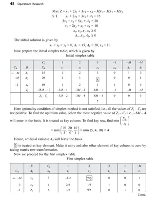
Example 36 Solve the problem
Max Z = 6x1 + 8x2
S.T. 5x1 + 10x2 £ 60
4x1 + 4x2 £ 40
x1, x2 ≥ 0
(a) Check whether the addition of constraint 7x1 + 2x2 £ 65 affects the optimality. If it does,
find the new optimum solution.
(b) Check whether the addition of the constraint 6x1 + 3x2 £ 48 affects the optimality. If it
does, find the new solution.
Form simplex method, the optimum simplex table is given by](https://image.slidesharecdn.com/181sample-chapter-221017205802-782c7ea6/85/181_Sample-Chapter-pdf-53-320.jpg)
![86 Operations Research
Solution
Solve the problem by general simplex method. We have optimal simplex table.
Cj 6 8 0 0
CB B XB x1 x2 S1 S2
8 x2 2 0 1 1/5 –1/4
6 x1 8 1 0 –1/5 1/2
Zj 64 6 8
2
5
1
Zj – Cj 0 0
2
5
1
Here, all the values of Zj – Cj ≥ 0. Hence, optimum solution will exist. x1 = 8, x2 = 2, Max
Z = 64.
(a) Determination of Z3 – C3. The relative contribution of the new product P3 is computed by
the following formula.
Zj – Cj = Cj – [CB]
Technical coefficient
of optimal table w.r.t.
the basic varia
able
Constraint
coefficients of
new variable
È
Î
Í
Í
Í
˘
˚
˙
˙
˙
¥
È
Î
Í
Í
Í
˘
˘
˚
˙
˙
˙
= 20 – [8, 6]
1
5
1
4
1
5
1
2
6
5
-
-
È
Î
Í
Í
Í
Í
˘
˚
˙
˙
˙
˙
¥
È
Î
Í
˘
˚
˙ =
63
5
Since the value Z3 – C3 is greater than zero. The solution is not optimal. It means that the
inclusion of new product (new variable) in original problem changes the optimality.
(b) Optimization of the modified problem. The constraint coefficients of the new variable X3
are determined using the following formula.
Revised constraint
coefficient of the
new variable
È
Î
Í
Í
Í
˘
˚
˙
˙
˙
=
Technical coefficient
of optimal table w.r.t.
the basic varia
able
Constraint coefficients
of new variable
È
Î
Í
Í
Í
˘
˚
˙
˙
˙
¥
È
Î
Í
˘
˘
˚
˙
=
1
5
1
4
1
5
1
2
6
5
-
-
È
Î
Í
Í
Í
Í
˘
˚
˙
˙
˙
˙
¥
È
Î
Í
˘
˚
˙ =
-
È
Î
Í
Í
Í
Í
˘
˚
˙
˙
˙
˙
1
20
13
10](https://image.slidesharecdn.com/181sample-chapter-221017205802-782c7ea6/85/181_Sample-Chapter-pdf-55-320.jpg)


![[OOP - Lec 02] Why do we need OOP](https://cdn.slidesharecdn.com/ss_thumbnails/lecture-02whydoweneedoop-160604054425-thumbnail.jpg?width=640&height=640&fit=bounds)