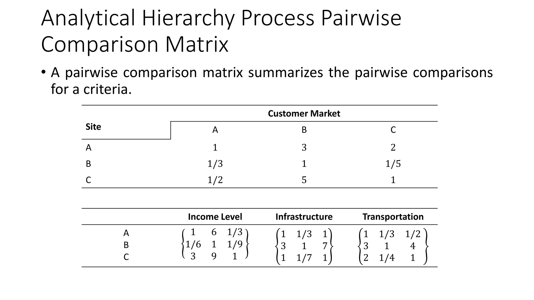
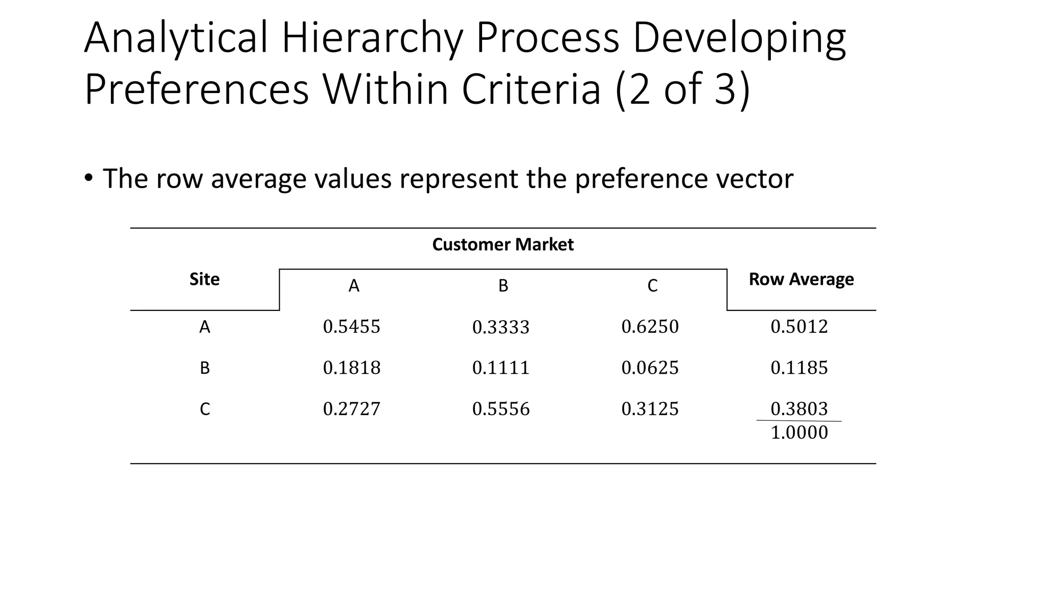
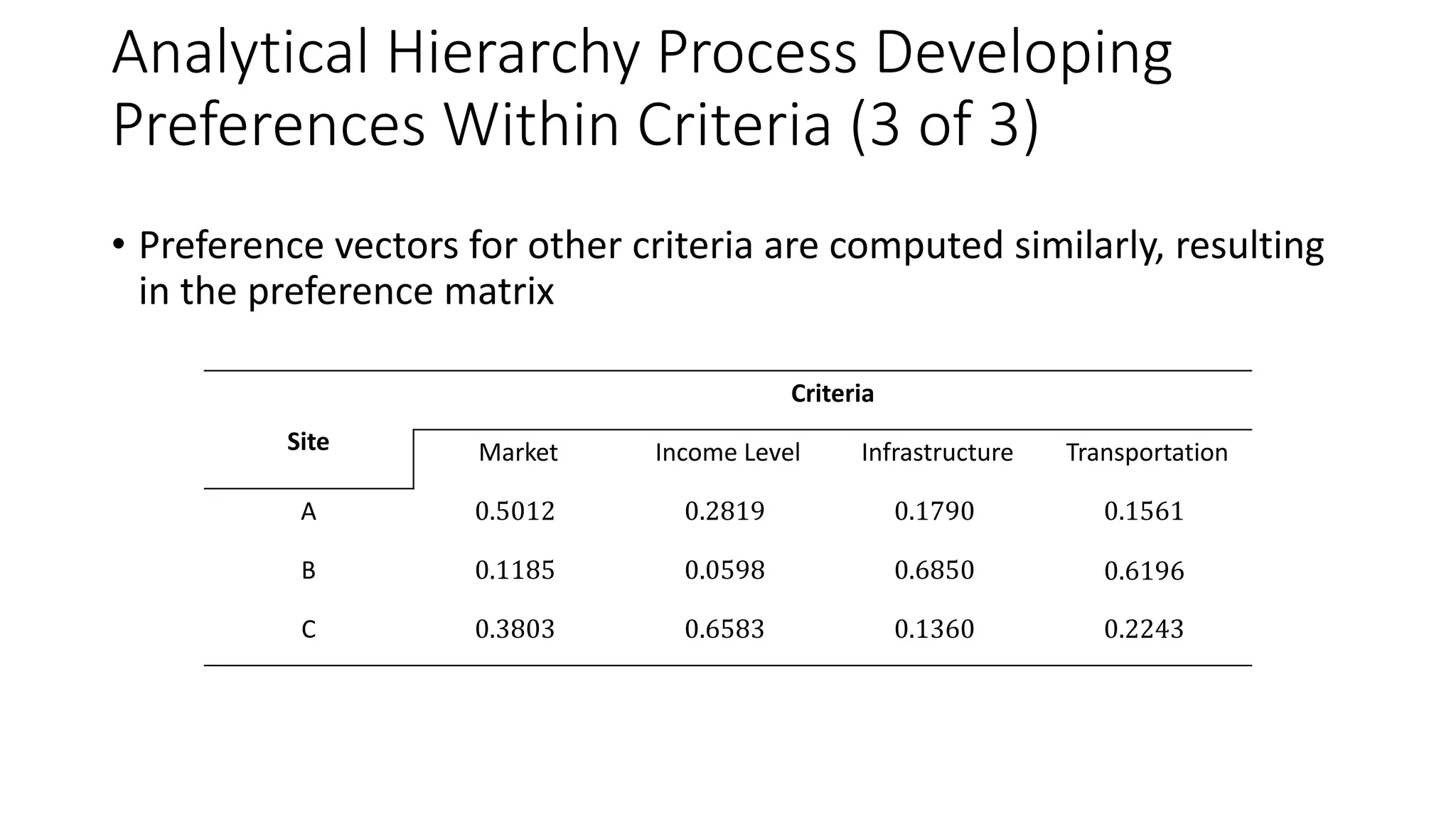
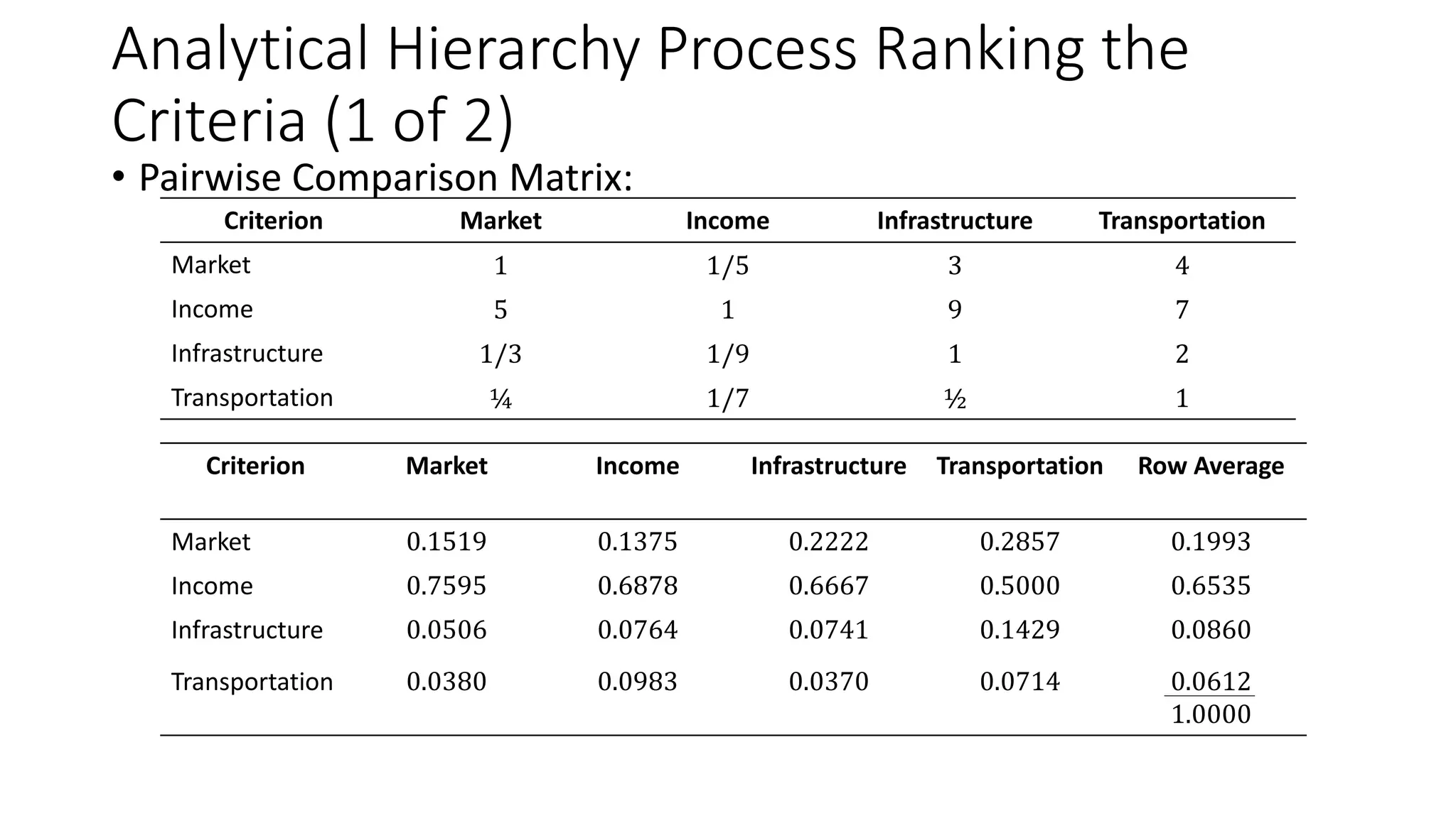
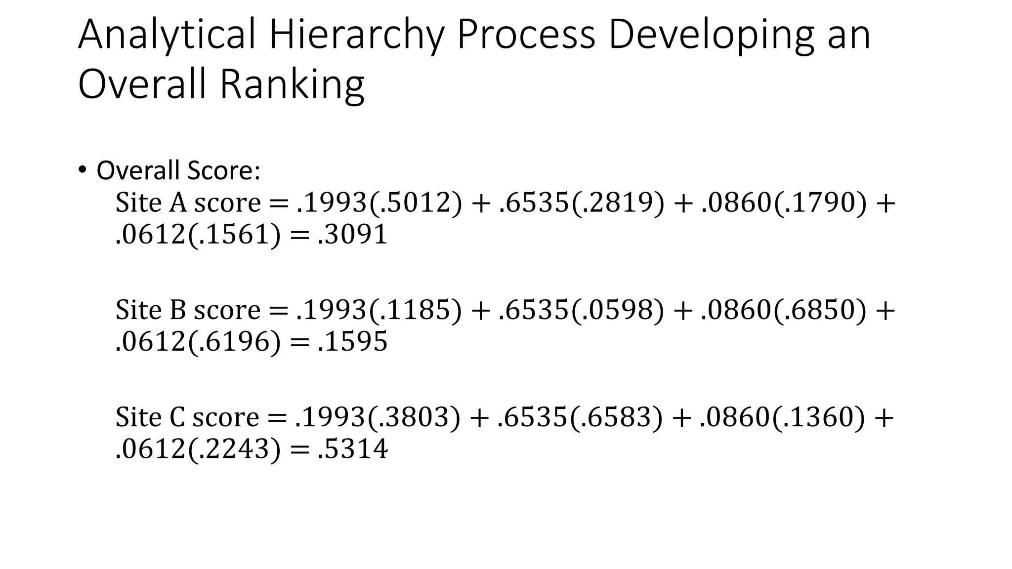
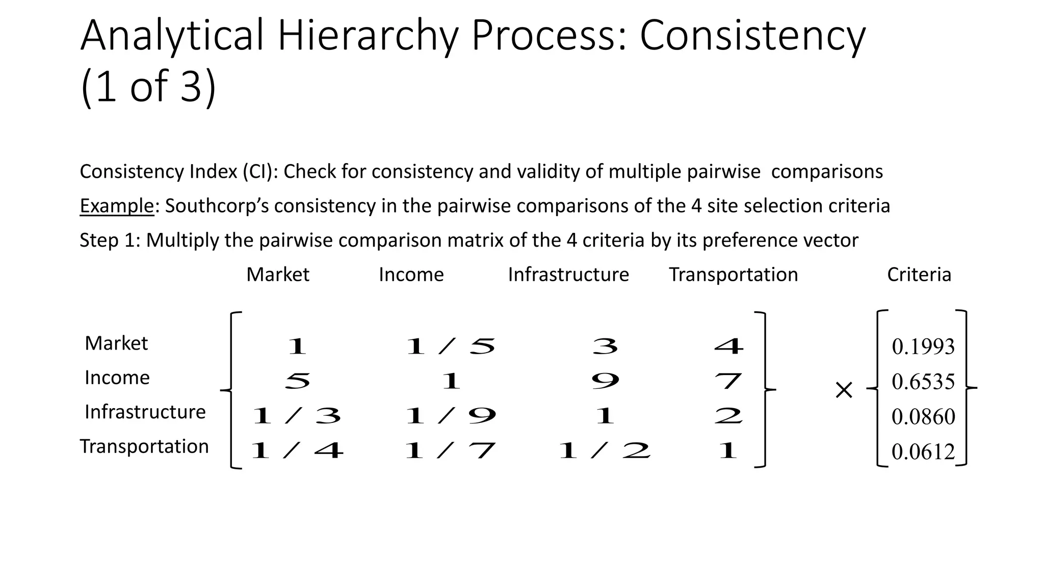
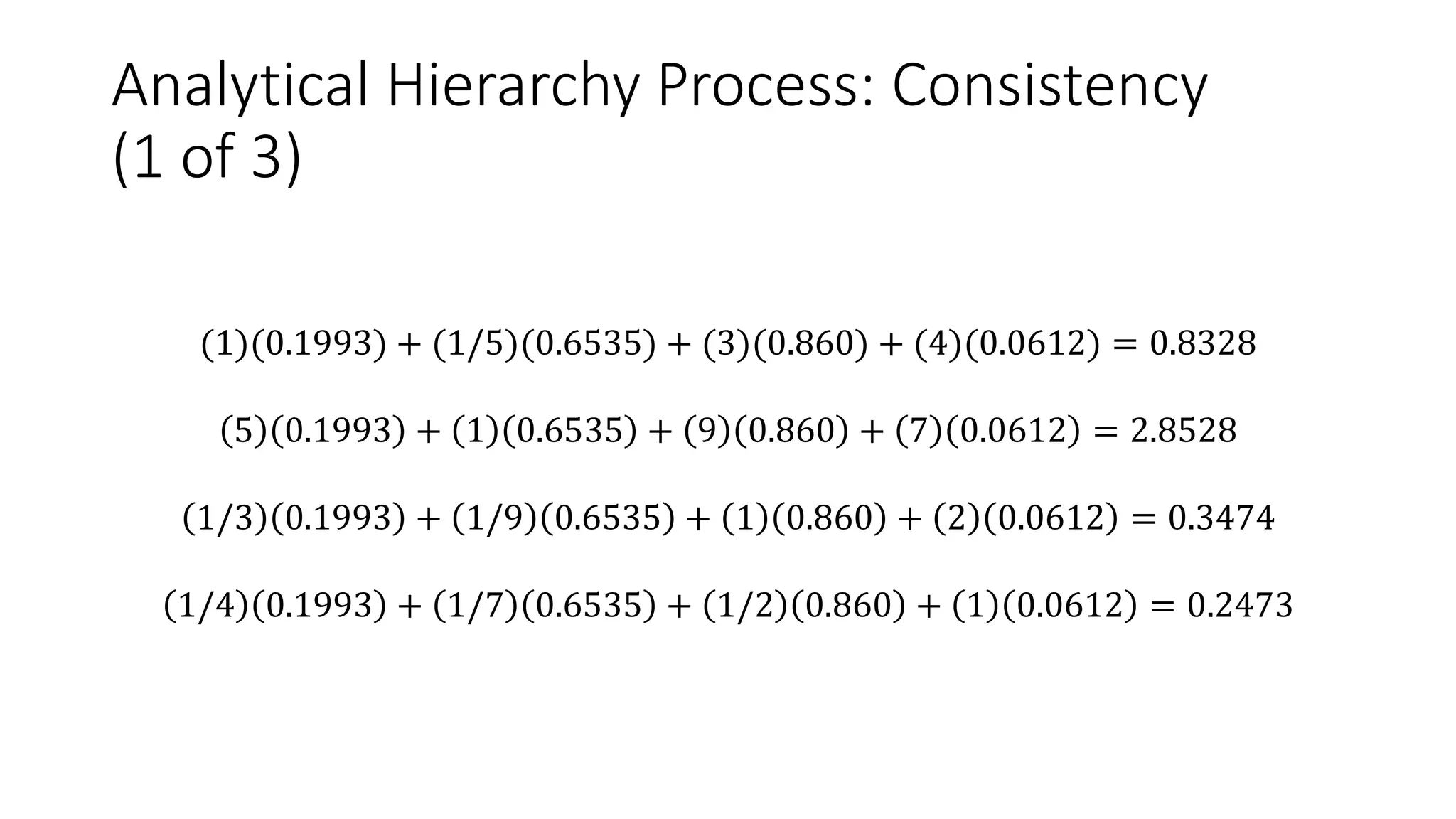
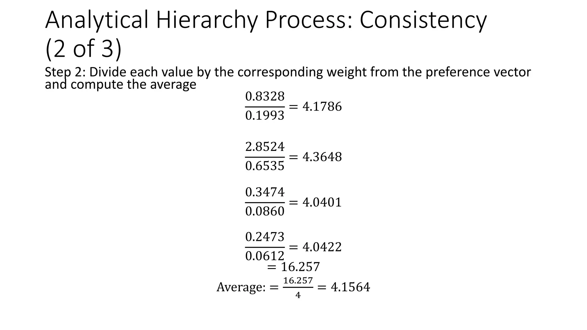
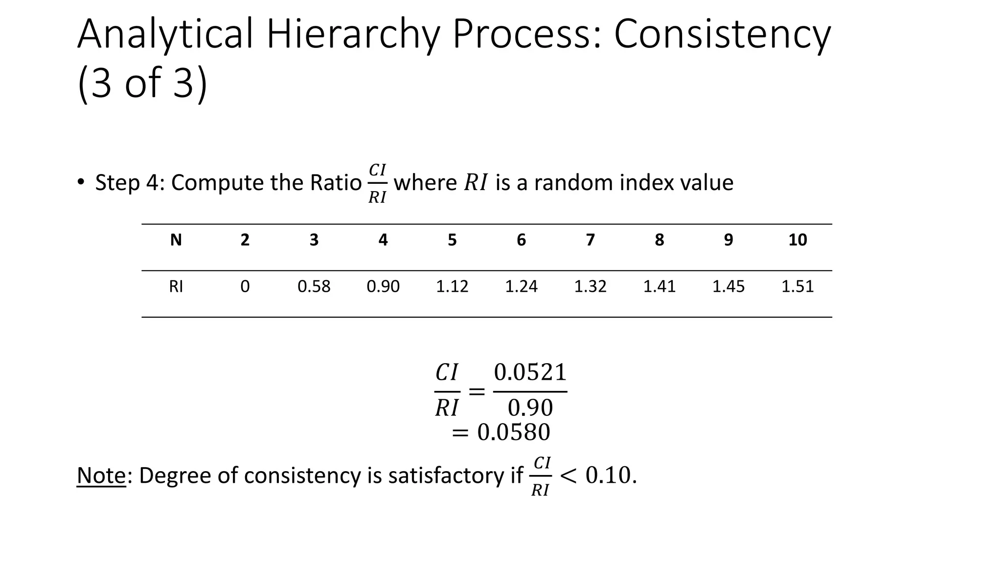
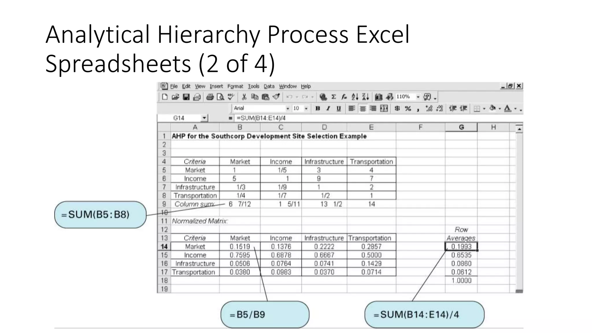
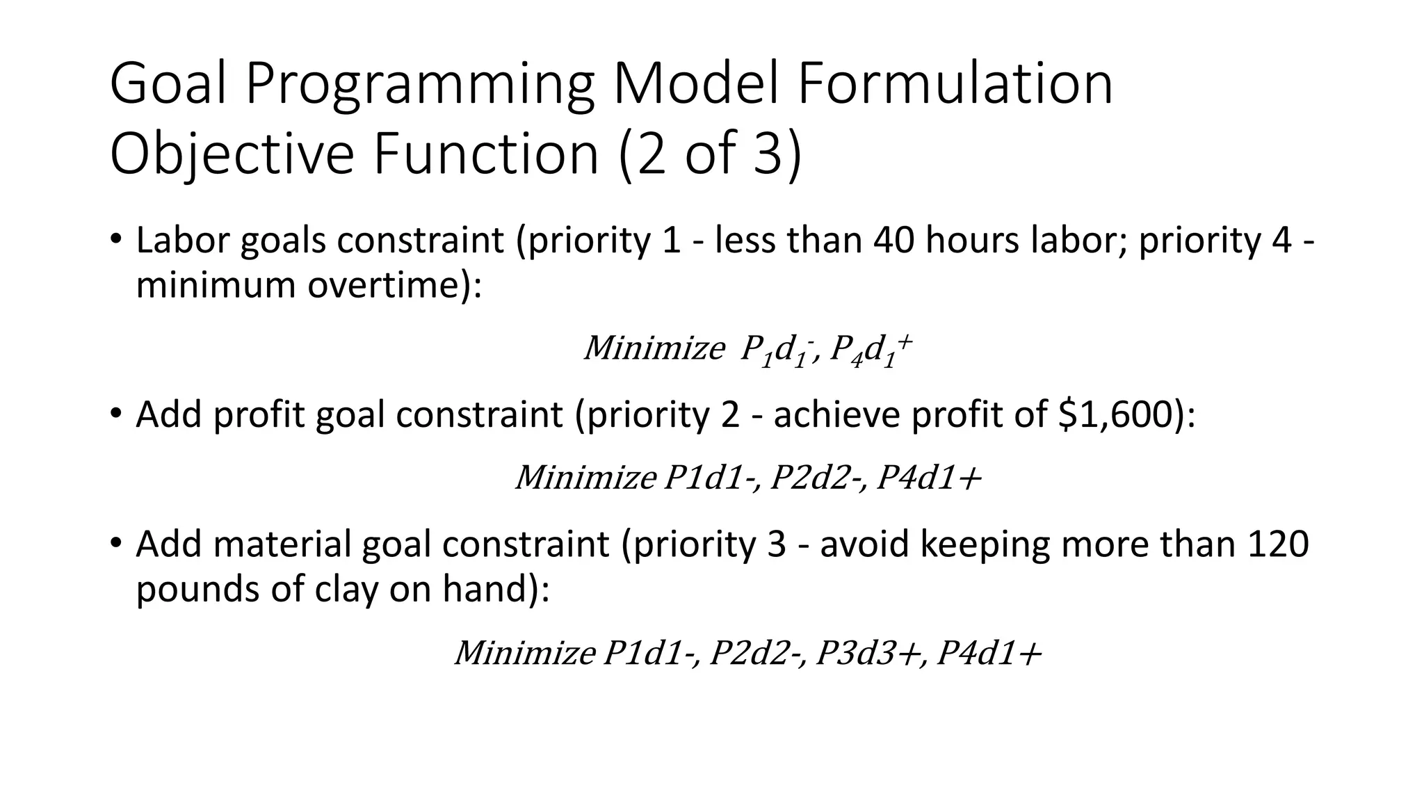
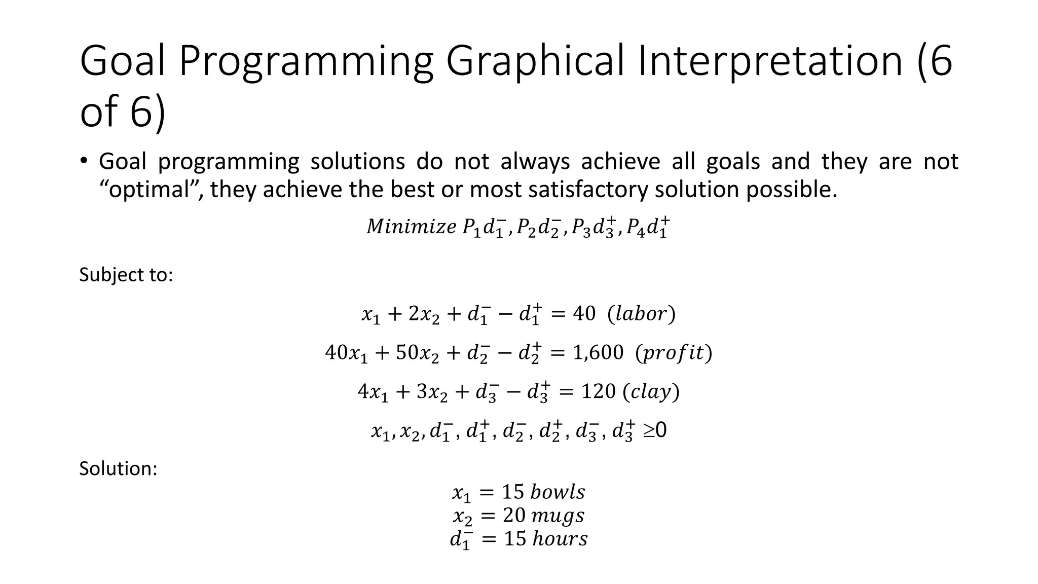
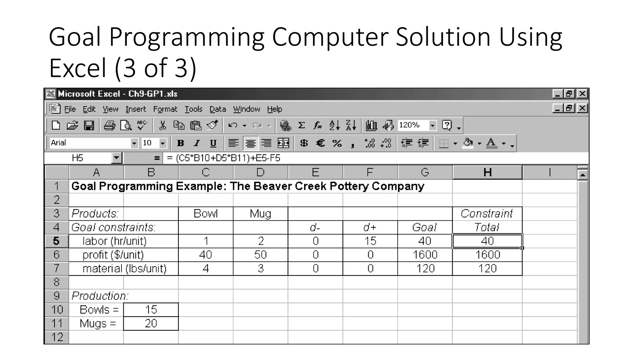
Analytical Hierarchy Process
(AHP)
Analytical Hierarchy Process (AHP)
• AHP is a method for ranking several decision alternatives and
selecting the best one when the decision maker has multiple
objectives, or criteria, on which to base the decision.
• The decision maker makes a decision based on how the alternatives
compare according to several criteria.
• The decision maker will select the alternative that best meets his or
her decision criteria.
• AHP is a process for developing a numerical score to rank each
decision alternative based on how well the alternative meets the
decision maker’s criteria.
AHP Example
• Southcorp Development Company shopping mall site selection.
• Three potential sites:
• Atlanta
• Birmingham
• Charlotte.
AHP Example
• Criteria for site comparisons:
• Customer market base.
• Income level
• Infrastructure
• Transportation
Analytical Hierarchy Process Hierarchy
Structure
• Top of the hierarchy: the objective (select the best site).
• Second level: how the four criteria contribute to the objective.
• Third level: how each of the three alternatives contributes to each of
the four criteria.
Analytical Hierarchy Process General
Mathematical Process
• Mathematically determine preferences for sites with respect to each
criterion.
• Mathematically determine preferences for criteria (rank order of
importance).
• Combine these two sets of preferences to mathematically derive a
composite score for each site.
• Select the site with the highest score.
Analytical Hierarchy Process Pairwise Comparisons
(1 of 2)
• In a pairwise comparison, two alternatives are compared according to
a criterion and one is preferred.
• A preference scale assigns numerical values to different levels of
performance.
Analytical Hierarchy Process Pairwise Comparisons
(2 of 2)
Preference Level Numerical Value
Equally preferred 1
Equally to moderately preferred 2
Moderately preferred 3
Moderately to strongly preferred 4
Strongly preferred 5
Strongly to very strongly preferred 6
Very strongly preferred 7
Very strongly to extremely preferred 8
Extremely preferred 9
Analytical Hierarchy Process Pairwise
Comparison Matrix
• A pairwise comparison matrix summarizes the pairwise comparisons
for a criteria.
Site
Customer Market
A B C
A 1 3 2
B 1/3 1 1/5
C 1/2 5 1
Income Level Infrastructure Transportation
A
B
C
1 6 1/3
1/6 1 1/9
3 9 1
1 1/3 1
3 1 7
1 1/7 1
1 1/3 1/2
3 1 4
2 1/4 1
Analytical Hierarchy Process Developing
Preferences Within Criteria (1 of 3)
• In synthetization, decision alternatives are prioritized with each
criterion and then normalized:
Customer Market
Site A B C
A
B
C
1
1/3
1/2
11/6
3
1
5
9
2
1/5
1
16/5
Customer Market
Site A B C
A
B
C
6/11
2/11
3/11
3/9
1/9
5/9
5/8
1/16
5/16
Analytical Hierarchy Process Developing
Preferences Within Criteria (2 of 3)
• The row average values represent the preference vector
Site
Customer Market
Row AverageA B C
A 0.5455 0.3333 0.6250 0.5012
B 0.1818 0.1111 0.0625 0.1185
C 0.2727 0.5556 0.3125 0.3803
1.0000
Analytical Hierarchy Process Developing
Preferences Within Criteria (3 of 3)
• Preference vectors for other criteria are computed similarly, resulting
in the preference matrix
Site
Criteria
Market Income Level Infrastructure Transportation
A 0.5012 0.2819 0.1790 0.1561
B 0.1185 0.0598 0.6850 0.6196
C 0.3803 0.6583 0.1360 0.2243
Analytical Hierarchy Process Ranking the
Criteria (1 of 2)
• Pairwise Comparison Matrix:
Criterion Market Income Infrastructure Transportation
Market 1 1/5 3 4
Income 5 1 9 7
Infrastructure 1/3 1/9 1 2
Transportation ¼ 1/7 ½ 1
Criterion Market Income Infrastructure Transportation Row Average
Market 0.1519 0.1375 0.2222 0.2857 0.1993
Income 0.7595 0.6878 0.6667 0.5000 0.6535
Infrastructure 0.0506 0.0764 0.0741 0.1429 0.0860
Transportation 0.0380 0.0983 0.0370 0.0714 0.0612
1.0000
Analytical Hierarchy Process Ranking the
Criteria (2 of 2)
• Preference Vector for Criteria:
0.1993
0.6535
0.0860
0.0612
Criterion
Market
Income
Infrastructure
Transportation
Analytical Hierarchy Process Developing an
Overall Ranking
• Overall Score:
Site A score = .1993(.5012) + .6535(.2819) + .0860(.1790) +
.0612(.1561) = .3091
Site B score = .1993(.1185) + .6535(.0598) + .0860(.6850) +
.0612(.6196) = .1595
Site C score = .1993(.3803) + .6535(.6583) + .0860(.1360) +
.0612(.2243) = .5314
Analytical Hierarchy Process Developing an Overall
Ranking
• Overall Ranking:
Site Score
Charlotte
Atlanta
Birmingham
0.5314
0.3091
0.1595
1.0000
Analytical Hierarchy Process Summary of
Mathematical Steps
• Develop a pairwise comparison matrix for each decision alternative
for each criteria.
• Synthetization
• Sum the values of each column of the pairwise comparison matrices.
• Divide each value in each column by the corresponding column sum.
• Average the values in each row of the normalized matrices.
• Combine the vectors of preferences for each criterion.
• Develop a pairwise comparison matrix for the criteria.
• Compute the normalized matrix.
• Develop the preference vector.
• Compute an overall score for each decision alternative
• Rank the decision alternatives.
Analytical Hierarchy Process: Consistency
(1 of 3)
Consistency Index (CI): Check for consistency and validity of multiple pairwise comparisons
Example: Southcorp’s consistency in the pairwise comparisons of the 4 site selection criteria
Step 1: Multiply the pairwise comparison matrix of the 4 criteria by its preference vector
Market Income Infrastructure Transportation Criteria
Market
Income
Infrastructure
Transportation
1 1 / 5 3 4
5 1 9 7
1 / 3 1 / 9 1 2
1 / 4 1 / 7 1 / 2 1
0.1993
0.6535
0.0860
0.0612
×
Analytical Hierarchy Process: Consistency
(1 of 3)
(1)(0.1993) + (1/5)(0.6535) + (3)(0.860) + (4)(0.0612) = 0.8328
5 0.1993 + 1 0.6535 + 9 0.860 + 7 0.0612 = 2.8528
1/3 0.1993 + 1/9 0.6535 + 1 0.860 + 2 0.0612 = 0.3474
1/4 0.1993 + 1/7 0.6535 + 1/2 0.860 + 1 0.0612 = 0.2473
Analytical Hierarchy Process: Consistency
(2 of 3)
Step 2: Divide each value by the corresponding weight from the preference vector
and compute the average
0.8328
0.1993
= 4.1786
2.8524
0.6535
= 4.3648
0.3474
0.0860
= 4.0401
0.2473
0.0612
= 4.0422
= 16.257
Average: =
16.257
4
= 4.1564
Analytical Hierarchy Process: Consistency
(2 of 3)
Step 3: Calculate the Consistency Index (CI)
𝐶𝐼 =
𝐴𝑣𝑒𝑟𝑎𝑔𝑒 − 𝑛
𝑛 − 1
, 𝑤ℎ𝑒𝑟𝑒 𝑛 𝑖𝑠 𝑛𝑜. 𝑜𝑓 𝑖𝑡𝑒𝑚𝑠 𝑐𝑜𝑚𝑝𝑎𝑟𝑒𝑑
𝐶𝐼 =
4.1564−4
4−1
= 0.0521
𝐶𝐼 = 0 𝑖𝑛𝑑𝑖𝑐𝑎𝑡𝑒𝑠 𝑝𝑒𝑟𝑓𝑒𝑐𝑡 𝑐𝑜𝑛𝑠𝑖𝑠𝑡𝑒𝑛𝑐𝑦
Analytical Hierarchy Process: Consistency
(3 of 3)
• Step 4: Compute the Ratio
𝐶𝐼
𝑅𝐼
where 𝑅𝐼 is a random index value
𝐶𝐼
𝑅𝐼
=
0.0521
0.90
= 0.0580
Note: Degree of consistency is satisfactory if
𝐶𝐼
𝑅𝐼
< 0.10.
N 2 3 4 5 6 7 8 9 10
RI 0 0.58 0.90 1.12 1.24 1.32 1.41 1.45 1.51
Analytical Hierarchy Process Excel
Spreadsheets (1 of 4)
Analytical Hierarchy Process Excel
Spreadsheets (2 of 4)
Analytical Hierarchy Process Excel
Spreadsheets (3 of 4)
Analytical Hierarchy Process Excel
Spreadsheets (4 of 4)
Goal Programming
• Goal programming is a variation of linear programming considering
more than one objective (goals) in the objective function.
Goal Programming Example
• Beaver Creek Pottery Company Example:
𝑀𝑎𝑥𝑖𝑚𝑖𝑧𝑒 𝑍 = 40𝑥1 + 50𝑋2
Subject to:
1𝑥1 + 2𝑥2 ≤ 40, ℎ𝑜𝑢𝑟𝑠 𝑜𝑓 𝑙𝑎𝑏𝑜𝑟
4𝑥1 + 3𝑥2 ≤ 120, 𝑝𝑜𝑢𝑛𝑑𝑠 𝑜𝑓 𝑐𝑙𝑎𝑦
𝑥1, 𝑥2 ≥ 0
Where:
𝑥1 = 𝑛𝑢𝑚𝑏𝑒𝑟 𝑜𝑓 𝑏𝑜𝑤𝑙𝑠 𝑝𝑟𝑜𝑑𝑢𝑐𝑒𝑑
𝑥2 = 𝑛𝑢𝑚𝑏𝑒𝑟 𝑜𝑓 𝑚𝑢𝑔𝑠 𝑝𝑟𝑜𝑑𝑢𝑐𝑒𝑑
Goal Programming Example
• Adding objectives (goals) in order of importance, the company:
• Does not want to use fewer than 40 hours of labor per day.
• Would like to achieve a satisfactory profit level of $1,600 per
day.
• Prefers not to keep more than 120 pounds of clay on hand each
day.
• Would like to minimize the amount of overtime.
Goal Programming Goal Constraint
Requirements
• All goal constraints are equalities that include deviational variables d- and
d+.
• A positive deviational variable (d+) is the amount by which a goal level is
exceeded.
• A negative deviation variable (d-) is the amount by which a goal level is
underachieved.
• At least one or both deviational variables in a goal constraint must equal
zero.
• The objective function in a goal programming model seeks to minimize the
deviation from the respective goals in the order of the goal priorities.
Goal Programming Model Formulation Goal
Constraints (1 of 3)
• Labor goal:
𝑥1 + 2𝑥2 + 𝑑1
−
− 𝑑1
+
= 40 (
ℎ𝑜𝑢𝑟𝑠
𝑑𝑎𝑦
)
• Profit goal:
40𝑥1 + 50𝑥2 + 𝑑2
−
− 𝑑2
+
= 1,600
$
𝑑𝑎𝑦
• Material goal:
4𝑥1 + 3𝑥2 + 𝑑3
−
− 𝑑3
+
= 120
(𝑙𝑏𝑠 𝑜𝑓 𝑐𝑙𝑎𝑦)
𝑑𝑎𝑦
Goal Programming Model Formulation
Objective Function (2 of 3)
• Labor goals constraint (priority 1 - less than 40 hours labor; priority 4 -
minimum overtime):
Minimize P1d1
-, P4d1
+
• Add profit goal constraint (priority 2 - achieve profit of $1,600):
Minimize P1d1-, P2d2-, P4d1+
• Add material goal constraint (priority 3 - avoid keeping more than 120
pounds of clay on hand):
Minimize P1d1-, P2d2-, P3d3+, P4d1+
Goal Programming Model Formulation
Complete Model (3 of 3)
• Complete Goal Programming Model:
𝑀𝑖𝑛𝑖𝑚𝑖𝑧𝑒 𝑃1 𝑑1
−
, 𝑃2 𝑑2
−
, 𝑃3 𝑑3
+
, 𝑃4 𝑑1
+
Subject to:
𝑥1 + 2𝑥2 + 𝑑1
−
− 𝑑1
+
= 40 (𝑙𝑎𝑏𝑜𝑟)
40𝑥1 + 50𝑥2 + 𝑑2
−
− 𝑑2
+
= 1,600 (𝑝𝑟𝑜𝑓𝑖𝑡)
4𝑥1 + 3𝑥2 + 𝑑3
−
− 𝑑3
+
= 120 (𝑐𝑙𝑎𝑦)
𝑥1, 𝑥2, 𝑑1
−
, 𝑑1
+
, 𝑑2
−
, 𝑑2
+
, 𝑑3
−
, 𝑑3
+
0
Goal Programming Graphical Interpretation (1
of 6)
𝑀𝑖𝑛𝑖𝑚𝑖𝑧𝑒 𝑃1 𝑑1
−
, 𝑃2 𝑑2
−
, 𝑃3 𝑑3
+
, 𝑃4 𝑑1
+
Subject to:
𝑥1 + 2𝑥2 + 𝑑1
−
− 𝑑1
+
= 40 (𝑙𝑎𝑏𝑜𝑟)
40𝑥1 + 50𝑥2 + 𝑑2
−
− 𝑑2
+
= 1,600 (𝑝𝑟𝑜𝑓𝑖𝑡)
4𝑥1 + 3𝑥2 + 𝑑3
−
− 𝑑3
+
= 120 (𝑐𝑙𝑎𝑦)
𝑥1, 𝑥2, 𝑑1
−
, 𝑑1
+
, 𝑑2
−
, 𝑑2
+
, 𝑑3
−
, 𝑑3
+
0
Goal Programming Graphical Interpretation (2
of 6)
𝑀𝑖𝑛𝑖𝑚𝑖𝑧𝑒 𝑃1 𝑑1
−
, 𝑃2 𝑑2
−
, 𝑃3 𝑑3
+
, 𝑃4 𝑑1
+
Subject to:
𝑥1 + 2𝑥2 + 𝑑1
−
− 𝑑1
+
= 40 (𝑙𝑎𝑏𝑜𝑟)
40𝑥1 + 50𝑥2 + 𝑑2
−
− 𝑑2
+
= 1,600 (𝑝𝑟𝑜𝑓𝑖𝑡)
4𝑥1 + 3𝑥2 + 𝑑3
−
− 𝑑3
+
= 120 (𝑐𝑙𝑎𝑦)
𝑥1, 𝑥2, 𝑑1
−
, 𝑑1
+
, 𝑑2
−
, 𝑑2
+
, 𝑑3
−
, 𝑑3
+
0
Goal Programming Graphical Interpretation (3
of 6)
𝑀𝑖𝑛𝑖𝑚𝑖𝑧𝑒 𝑃1 𝑑1
−
, 𝑃2 𝑑2
−
, 𝑃3 𝑑3
+
, 𝑃4 𝑑1
+
Subject to:
𝑥1 + 2𝑥2 + 𝑑1
−
− 𝑑1
+
= 40 (𝑙𝑎𝑏𝑜𝑟)
40𝑥1 + 50𝑥2 + 𝑑2
−
− 𝑑2
+
= 1,600 (𝑝𝑟𝑜𝑓𝑖𝑡)
4𝑥1 + 3𝑥2 + 𝑑3
−
− 𝑑3
+
= 120 (𝑐𝑙𝑎𝑦)
𝑥1, 𝑥2, 𝑑1
−
, 𝑑1
+
, 𝑑2
−
, 𝑑2
+
, 𝑑3
−
, 𝑑3
+
0
Goal Programming Graphical Interpretation (4
of 6)
𝑀𝑖𝑛𝑖𝑚𝑖𝑧𝑒 𝑃1 𝑑1
−
, 𝑃2 𝑑2
−
, 𝑃3 𝑑3
+
, 𝑃4 𝑑1
+
Subject to:
𝑥1 + 2𝑥2 + 𝑑1
−
− 𝑑1
+
= 40 (𝑙𝑎𝑏𝑜𝑟)
40𝑥1 + 50𝑥2 + 𝑑2
−
− 𝑑2
+
= 1,600 (𝑝𝑟𝑜𝑓𝑖𝑡)
4𝑥1 + 3𝑥2 + 𝑑3
−
− 𝑑3
+
= 120 (𝑐𝑙𝑎𝑦)
𝑥1, 𝑥2, 𝑑1
−
, 𝑑1
+
, 𝑑2
−
, 𝑑2
+
, 𝑑3
−
, 𝑑3
+
0
Goal Programming Graphical Interpretation (5
of 6)
𝑀𝑖𝑛𝑖𝑚𝑖𝑧𝑒 𝑃1 𝑑1
−
, 𝑃2 𝑑2
−
, 𝑃3 𝑑3
+
, 𝑃4 𝑑1
+
Subject to:
𝑥1 + 2𝑥2 + 𝑑1
−
− 𝑑1
+
= 40 (𝑙𝑎𝑏𝑜𝑟)
40𝑥1 + 50𝑥2 + 𝑑2
−
− 𝑑2
+
= 1,600 (𝑝𝑟𝑜𝑓𝑖𝑡)
4𝑥1 + 3𝑥2 + 𝑑3
−
− 𝑑3
+
= 120 (𝑐𝑙𝑎𝑦)
𝑥1, 𝑥2, 𝑑1
−
, 𝑑1
+
, 𝑑2
−
, 𝑑2
+
, 𝑑3
−
, 𝑑3
+
0
Goal Programming Graphical Interpretation (6
of 6)
• Goal programming solutions do not always achieve all goals and they are not
“optimal”, they achieve the best or most satisfactory solution possible.
𝑀𝑖𝑛𝑖𝑚𝑖𝑧𝑒 𝑃1 𝑑1
−
, 𝑃2 𝑑2
−
, 𝑃3 𝑑3
+
, 𝑃4 𝑑1
+
Subject to:
𝑥1 + 2𝑥2 + 𝑑1
−
− 𝑑1
+
= 40 (𝑙𝑎𝑏𝑜𝑟)
40𝑥1 + 50𝑥2 + 𝑑2
−
− 𝑑2
+
= 1,600 (𝑝𝑟𝑜𝑓𝑖𝑡)
4𝑥1 + 3𝑥2 + 𝑑3
−
− 𝑑3
+
= 120 (𝑐𝑙𝑎𝑦)
𝑥1, 𝑥2, 𝑑1
−
, 𝑑1
+
, 𝑑2
−
, 𝑑2
+
, 𝑑3
−
, 𝑑3
+
0
Solution:
𝑥1 = 15 𝑏𝑜𝑤𝑙𝑠
𝑥2 = 20 𝑚𝑢𝑔𝑠
𝑑1
−
= 15 ℎ𝑜𝑢𝑟𝑠
Goal Programming Computer Solution Using
Excel (1 of 3)
Goal Programming Computer Solution Using
Excel (2 of 3)
Goal Programming Computer Solution Using
Excel (3 of 3)

Ahp

  • 1.
  • 2.
    Analytical Hierarchy Process(AHP) • AHP is a method for ranking several decision alternatives and selecting the best one when the decision maker has multiple objectives, or criteria, on which to base the decision. • The decision maker makes a decision based on how the alternatives compare according to several criteria. • The decision maker will select the alternative that best meets his or her decision criteria. • AHP is a process for developing a numerical score to rank each decision alternative based on how well the alternative meets the decision maker’s criteria.
  • 3.
    AHP Example • SouthcorpDevelopment Company shopping mall site selection. • Three potential sites: • Atlanta • Birmingham • Charlotte.
  • 4.
    AHP Example • Criteriafor site comparisons: • Customer market base. • Income level • Infrastructure • Transportation
  • 5.
    Analytical Hierarchy ProcessHierarchy Structure • Top of the hierarchy: the objective (select the best site). • Second level: how the four criteria contribute to the objective. • Third level: how each of the three alternatives contributes to each of the four criteria.
  • 6.
    Analytical Hierarchy ProcessGeneral Mathematical Process • Mathematically determine preferences for sites with respect to each criterion. • Mathematically determine preferences for criteria (rank order of importance). • Combine these two sets of preferences to mathematically derive a composite score for each site. • Select the site with the highest score.
  • 7.
    Analytical Hierarchy ProcessPairwise Comparisons (1 of 2) • In a pairwise comparison, two alternatives are compared according to a criterion and one is preferred. • A preference scale assigns numerical values to different levels of performance.
  • 8.
    Analytical Hierarchy ProcessPairwise Comparisons (2 of 2) Preference Level Numerical Value Equally preferred 1 Equally to moderately preferred 2 Moderately preferred 3 Moderately to strongly preferred 4 Strongly preferred 5 Strongly to very strongly preferred 6 Very strongly preferred 7 Very strongly to extremely preferred 8 Extremely preferred 9
  • 9.
    Analytical Hierarchy ProcessPairwise Comparison Matrix • A pairwise comparison matrix summarizes the pairwise comparisons for a criteria. Site Customer Market A B C A 1 3 2 B 1/3 1 1/5 C 1/2 5 1 Income Level Infrastructure Transportation A B C 1 6 1/3 1/6 1 1/9 3 9 1 1 1/3 1 3 1 7 1 1/7 1 1 1/3 1/2 3 1 4 2 1/4 1
  • 10.
    Analytical Hierarchy ProcessDeveloping Preferences Within Criteria (1 of 3) • In synthetization, decision alternatives are prioritized with each criterion and then normalized: Customer Market Site A B C A B C 1 1/3 1/2 11/6 3 1 5 9 2 1/5 1 16/5 Customer Market Site A B C A B C 6/11 2/11 3/11 3/9 1/9 5/9 5/8 1/16 5/16
  • 11.
    Analytical Hierarchy ProcessDeveloping Preferences Within Criteria (2 of 3) • The row average values represent the preference vector Site Customer Market Row AverageA B C A 0.5455 0.3333 0.6250 0.5012 B 0.1818 0.1111 0.0625 0.1185 C 0.2727 0.5556 0.3125 0.3803 1.0000
  • 12.
    Analytical Hierarchy ProcessDeveloping Preferences Within Criteria (3 of 3) • Preference vectors for other criteria are computed similarly, resulting in the preference matrix Site Criteria Market Income Level Infrastructure Transportation A 0.5012 0.2819 0.1790 0.1561 B 0.1185 0.0598 0.6850 0.6196 C 0.3803 0.6583 0.1360 0.2243
  • 13.
    Analytical Hierarchy ProcessRanking the Criteria (1 of 2) • Pairwise Comparison Matrix: Criterion Market Income Infrastructure Transportation Market 1 1/5 3 4 Income 5 1 9 7 Infrastructure 1/3 1/9 1 2 Transportation ¼ 1/7 ½ 1 Criterion Market Income Infrastructure Transportation Row Average Market 0.1519 0.1375 0.2222 0.2857 0.1993 Income 0.7595 0.6878 0.6667 0.5000 0.6535 Infrastructure 0.0506 0.0764 0.0741 0.1429 0.0860 Transportation 0.0380 0.0983 0.0370 0.0714 0.0612 1.0000
  • 14.
    Analytical Hierarchy ProcessRanking the Criteria (2 of 2) • Preference Vector for Criteria: 0.1993 0.6535 0.0860 0.0612 Criterion Market Income Infrastructure Transportation
  • 15.
    Analytical Hierarchy ProcessDeveloping an Overall Ranking • Overall Score: Site A score = .1993(.5012) + .6535(.2819) + .0860(.1790) + .0612(.1561) = .3091 Site B score = .1993(.1185) + .6535(.0598) + .0860(.6850) + .0612(.6196) = .1595 Site C score = .1993(.3803) + .6535(.6583) + .0860(.1360) + .0612(.2243) = .5314
  • 16.
    Analytical Hierarchy ProcessDeveloping an Overall Ranking • Overall Ranking: Site Score Charlotte Atlanta Birmingham 0.5314 0.3091 0.1595 1.0000
  • 17.
    Analytical Hierarchy ProcessSummary of Mathematical Steps • Develop a pairwise comparison matrix for each decision alternative for each criteria. • Synthetization • Sum the values of each column of the pairwise comparison matrices. • Divide each value in each column by the corresponding column sum. • Average the values in each row of the normalized matrices. • Combine the vectors of preferences for each criterion. • Develop a pairwise comparison matrix for the criteria. • Compute the normalized matrix. • Develop the preference vector. • Compute an overall score for each decision alternative • Rank the decision alternatives.
  • 18.
    Analytical Hierarchy Process:Consistency (1 of 3) Consistency Index (CI): Check for consistency and validity of multiple pairwise comparisons Example: Southcorp’s consistency in the pairwise comparisons of the 4 site selection criteria Step 1: Multiply the pairwise comparison matrix of the 4 criteria by its preference vector Market Income Infrastructure Transportation Criteria Market Income Infrastructure Transportation 1 1 / 5 3 4 5 1 9 7 1 / 3 1 / 9 1 2 1 / 4 1 / 7 1 / 2 1 0.1993 0.6535 0.0860 0.0612 ×
  • 19.
    Analytical Hierarchy Process:Consistency (1 of 3) (1)(0.1993) + (1/5)(0.6535) + (3)(0.860) + (4)(0.0612) = 0.8328 5 0.1993 + 1 0.6535 + 9 0.860 + 7 0.0612 = 2.8528 1/3 0.1993 + 1/9 0.6535 + 1 0.860 + 2 0.0612 = 0.3474 1/4 0.1993 + 1/7 0.6535 + 1/2 0.860 + 1 0.0612 = 0.2473
  • 20.
    Analytical Hierarchy Process:Consistency (2 of 3) Step 2: Divide each value by the corresponding weight from the preference vector and compute the average 0.8328 0.1993 = 4.1786 2.8524 0.6535 = 4.3648 0.3474 0.0860 = 4.0401 0.2473 0.0612 = 4.0422 = 16.257 Average: = 16.257 4 = 4.1564
  • 21.
    Analytical Hierarchy Process:Consistency (2 of 3) Step 3: Calculate the Consistency Index (CI) 𝐶𝐼 = 𝐴𝑣𝑒𝑟𝑎𝑔𝑒 − 𝑛 𝑛 − 1 , 𝑤ℎ𝑒𝑟𝑒 𝑛 𝑖𝑠 𝑛𝑜. 𝑜𝑓 𝑖𝑡𝑒𝑚𝑠 𝑐𝑜𝑚𝑝𝑎𝑟𝑒𝑑 𝐶𝐼 = 4.1564−4 4−1 = 0.0521 𝐶𝐼 = 0 𝑖𝑛𝑑𝑖𝑐𝑎𝑡𝑒𝑠 𝑝𝑒𝑟𝑓𝑒𝑐𝑡 𝑐𝑜𝑛𝑠𝑖𝑠𝑡𝑒𝑛𝑐𝑦
  • 22.
    Analytical Hierarchy Process:Consistency (3 of 3) • Step 4: Compute the Ratio 𝐶𝐼 𝑅𝐼 where 𝑅𝐼 is a random index value 𝐶𝐼 𝑅𝐼 = 0.0521 0.90 = 0.0580 Note: Degree of consistency is satisfactory if 𝐶𝐼 𝑅𝐼 < 0.10. N 2 3 4 5 6 7 8 9 10 RI 0 0.58 0.90 1.12 1.24 1.32 1.41 1.45 1.51
  • 23.
    Analytical Hierarchy ProcessExcel Spreadsheets (1 of 4)
  • 24.
    Analytical Hierarchy ProcessExcel Spreadsheets (2 of 4)
  • 25.
    Analytical Hierarchy ProcessExcel Spreadsheets (3 of 4)
  • 26.
    Analytical Hierarchy ProcessExcel Spreadsheets (4 of 4)
  • 27.
    Goal Programming • Goalprogramming is a variation of linear programming considering more than one objective (goals) in the objective function.
  • 28.
    Goal Programming Example •Beaver Creek Pottery Company Example: 𝑀𝑎𝑥𝑖𝑚𝑖𝑧𝑒 𝑍 = 40𝑥1 + 50𝑋2 Subject to: 1𝑥1 + 2𝑥2 ≤ 40, ℎ𝑜𝑢𝑟𝑠 𝑜𝑓 𝑙𝑎𝑏𝑜𝑟 4𝑥1 + 3𝑥2 ≤ 120, 𝑝𝑜𝑢𝑛𝑑𝑠 𝑜𝑓 𝑐𝑙𝑎𝑦 𝑥1, 𝑥2 ≥ 0 Where: 𝑥1 = 𝑛𝑢𝑚𝑏𝑒𝑟 𝑜𝑓 𝑏𝑜𝑤𝑙𝑠 𝑝𝑟𝑜𝑑𝑢𝑐𝑒𝑑 𝑥2 = 𝑛𝑢𝑚𝑏𝑒𝑟 𝑜𝑓 𝑚𝑢𝑔𝑠 𝑝𝑟𝑜𝑑𝑢𝑐𝑒𝑑
  • 29.
    Goal Programming Example •Adding objectives (goals) in order of importance, the company: • Does not want to use fewer than 40 hours of labor per day. • Would like to achieve a satisfactory profit level of $1,600 per day. • Prefers not to keep more than 120 pounds of clay on hand each day. • Would like to minimize the amount of overtime.
  • 30.
    Goal Programming GoalConstraint Requirements • All goal constraints are equalities that include deviational variables d- and d+. • A positive deviational variable (d+) is the amount by which a goal level is exceeded. • A negative deviation variable (d-) is the amount by which a goal level is underachieved. • At least one or both deviational variables in a goal constraint must equal zero. • The objective function in a goal programming model seeks to minimize the deviation from the respective goals in the order of the goal priorities.
  • 31.
    Goal Programming ModelFormulation Goal Constraints (1 of 3) • Labor goal: 𝑥1 + 2𝑥2 + 𝑑1 − − 𝑑1 + = 40 ( ℎ𝑜𝑢𝑟𝑠 𝑑𝑎𝑦 ) • Profit goal: 40𝑥1 + 50𝑥2 + 𝑑2 − − 𝑑2 + = 1,600 $ 𝑑𝑎𝑦 • Material goal: 4𝑥1 + 3𝑥2 + 𝑑3 − − 𝑑3 + = 120 (𝑙𝑏𝑠 𝑜𝑓 𝑐𝑙𝑎𝑦) 𝑑𝑎𝑦
  • 32.
    Goal Programming ModelFormulation Objective Function (2 of 3) • Labor goals constraint (priority 1 - less than 40 hours labor; priority 4 - minimum overtime): Minimize P1d1 -, P4d1 + • Add profit goal constraint (priority 2 - achieve profit of $1,600): Minimize P1d1-, P2d2-, P4d1+ • Add material goal constraint (priority 3 - avoid keeping more than 120 pounds of clay on hand): Minimize P1d1-, P2d2-, P3d3+, P4d1+
  • 33.
    Goal Programming ModelFormulation Complete Model (3 of 3) • Complete Goal Programming Model: 𝑀𝑖𝑛𝑖𝑚𝑖𝑧𝑒 𝑃1 𝑑1 − , 𝑃2 𝑑2 − , 𝑃3 𝑑3 + , 𝑃4 𝑑1 + Subject to: 𝑥1 + 2𝑥2 + 𝑑1 − − 𝑑1 + = 40 (𝑙𝑎𝑏𝑜𝑟) 40𝑥1 + 50𝑥2 + 𝑑2 − − 𝑑2 + = 1,600 (𝑝𝑟𝑜𝑓𝑖𝑡) 4𝑥1 + 3𝑥2 + 𝑑3 − − 𝑑3 + = 120 (𝑐𝑙𝑎𝑦) 𝑥1, 𝑥2, 𝑑1 − , 𝑑1 + , 𝑑2 − , 𝑑2 + , 𝑑3 − , 𝑑3 + 0
  • 34.
    Goal Programming GraphicalInterpretation (1 of 6) 𝑀𝑖𝑛𝑖𝑚𝑖𝑧𝑒 𝑃1 𝑑1 − , 𝑃2 𝑑2 − , 𝑃3 𝑑3 + , 𝑃4 𝑑1 + Subject to: 𝑥1 + 2𝑥2 + 𝑑1 − − 𝑑1 + = 40 (𝑙𝑎𝑏𝑜𝑟) 40𝑥1 + 50𝑥2 + 𝑑2 − − 𝑑2 + = 1,600 (𝑝𝑟𝑜𝑓𝑖𝑡) 4𝑥1 + 3𝑥2 + 𝑑3 − − 𝑑3 + = 120 (𝑐𝑙𝑎𝑦) 𝑥1, 𝑥2, 𝑑1 − , 𝑑1 + , 𝑑2 − , 𝑑2 + , 𝑑3 − , 𝑑3 + 0
  • 35.
    Goal Programming GraphicalInterpretation (2 of 6) 𝑀𝑖𝑛𝑖𝑚𝑖𝑧𝑒 𝑃1 𝑑1 − , 𝑃2 𝑑2 − , 𝑃3 𝑑3 + , 𝑃4 𝑑1 + Subject to: 𝑥1 + 2𝑥2 + 𝑑1 − − 𝑑1 + = 40 (𝑙𝑎𝑏𝑜𝑟) 40𝑥1 + 50𝑥2 + 𝑑2 − − 𝑑2 + = 1,600 (𝑝𝑟𝑜𝑓𝑖𝑡) 4𝑥1 + 3𝑥2 + 𝑑3 − − 𝑑3 + = 120 (𝑐𝑙𝑎𝑦) 𝑥1, 𝑥2, 𝑑1 − , 𝑑1 + , 𝑑2 − , 𝑑2 + , 𝑑3 − , 𝑑3 + 0
  • 36.
    Goal Programming GraphicalInterpretation (3 of 6) 𝑀𝑖𝑛𝑖𝑚𝑖𝑧𝑒 𝑃1 𝑑1 − , 𝑃2 𝑑2 − , 𝑃3 𝑑3 + , 𝑃4 𝑑1 + Subject to: 𝑥1 + 2𝑥2 + 𝑑1 − − 𝑑1 + = 40 (𝑙𝑎𝑏𝑜𝑟) 40𝑥1 + 50𝑥2 + 𝑑2 − − 𝑑2 + = 1,600 (𝑝𝑟𝑜𝑓𝑖𝑡) 4𝑥1 + 3𝑥2 + 𝑑3 − − 𝑑3 + = 120 (𝑐𝑙𝑎𝑦) 𝑥1, 𝑥2, 𝑑1 − , 𝑑1 + , 𝑑2 − , 𝑑2 + , 𝑑3 − , 𝑑3 + 0
  • 37.
    Goal Programming GraphicalInterpretation (4 of 6) 𝑀𝑖𝑛𝑖𝑚𝑖𝑧𝑒 𝑃1 𝑑1 − , 𝑃2 𝑑2 − , 𝑃3 𝑑3 + , 𝑃4 𝑑1 + Subject to: 𝑥1 + 2𝑥2 + 𝑑1 − − 𝑑1 + = 40 (𝑙𝑎𝑏𝑜𝑟) 40𝑥1 + 50𝑥2 + 𝑑2 − − 𝑑2 + = 1,600 (𝑝𝑟𝑜𝑓𝑖𝑡) 4𝑥1 + 3𝑥2 + 𝑑3 − − 𝑑3 + = 120 (𝑐𝑙𝑎𝑦) 𝑥1, 𝑥2, 𝑑1 − , 𝑑1 + , 𝑑2 − , 𝑑2 + , 𝑑3 − , 𝑑3 + 0
  • 38.
    Goal Programming GraphicalInterpretation (5 of 6) 𝑀𝑖𝑛𝑖𝑚𝑖𝑧𝑒 𝑃1 𝑑1 − , 𝑃2 𝑑2 − , 𝑃3 𝑑3 + , 𝑃4 𝑑1 + Subject to: 𝑥1 + 2𝑥2 + 𝑑1 − − 𝑑1 + = 40 (𝑙𝑎𝑏𝑜𝑟) 40𝑥1 + 50𝑥2 + 𝑑2 − − 𝑑2 + = 1,600 (𝑝𝑟𝑜𝑓𝑖𝑡) 4𝑥1 + 3𝑥2 + 𝑑3 − − 𝑑3 + = 120 (𝑐𝑙𝑎𝑦) 𝑥1, 𝑥2, 𝑑1 − , 𝑑1 + , 𝑑2 − , 𝑑2 + , 𝑑3 − , 𝑑3 + 0
  • 39.
    Goal Programming GraphicalInterpretation (6 of 6) • Goal programming solutions do not always achieve all goals and they are not “optimal”, they achieve the best or most satisfactory solution possible. 𝑀𝑖𝑛𝑖𝑚𝑖𝑧𝑒 𝑃1 𝑑1 − , 𝑃2 𝑑2 − , 𝑃3 𝑑3 + , 𝑃4 𝑑1 + Subject to: 𝑥1 + 2𝑥2 + 𝑑1 − − 𝑑1 + = 40 (𝑙𝑎𝑏𝑜𝑟) 40𝑥1 + 50𝑥2 + 𝑑2 − − 𝑑2 + = 1,600 (𝑝𝑟𝑜𝑓𝑖𝑡) 4𝑥1 + 3𝑥2 + 𝑑3 − − 𝑑3 + = 120 (𝑐𝑙𝑎𝑦) 𝑥1, 𝑥2, 𝑑1 − , 𝑑1 + , 𝑑2 − , 𝑑2 + , 𝑑3 − , 𝑑3 + 0 Solution: 𝑥1 = 15 𝑏𝑜𝑤𝑙𝑠 𝑥2 = 20 𝑚𝑢𝑔𝑠 𝑑1 − = 15 ℎ𝑜𝑢𝑟𝑠
  • 40.
    Goal Programming ComputerSolution Using Excel (1 of 3)
  • 41.
    Goal Programming ComputerSolution Using Excel (2 of 3)
  • 42.
    Goal Programming ComputerSolution Using Excel (3 of 3)