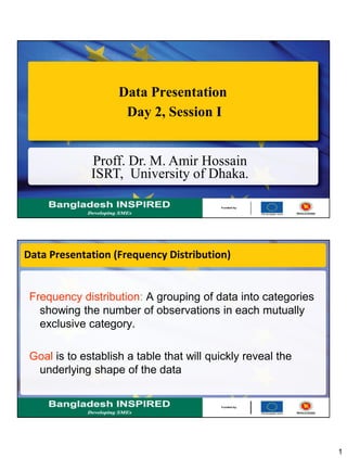
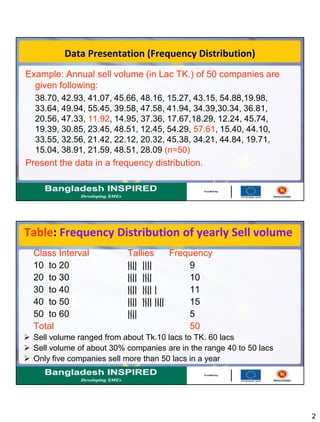
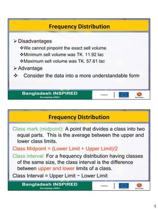
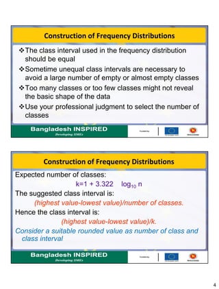
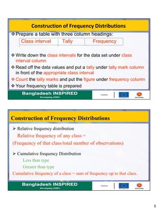
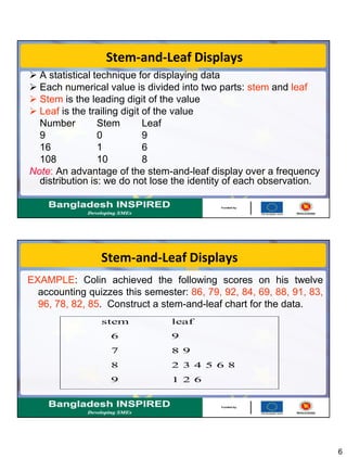
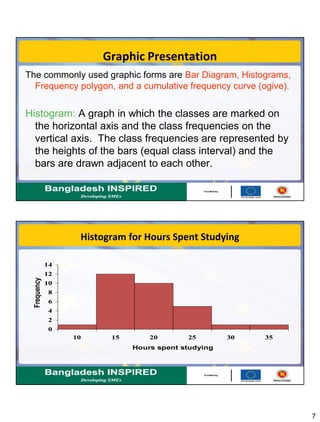
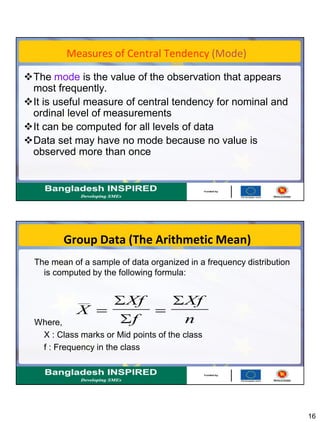
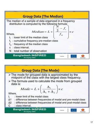
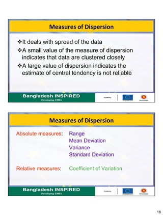
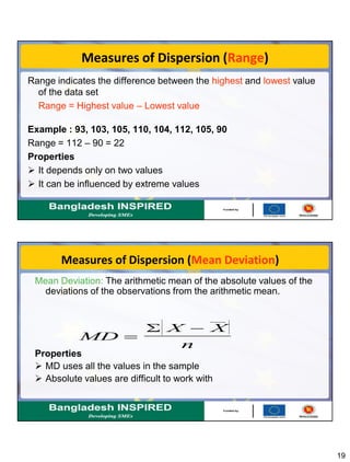
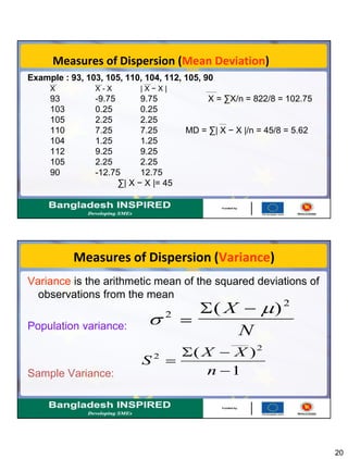
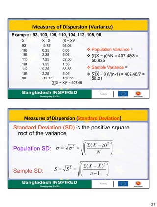
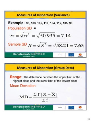
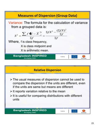
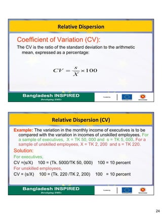
This document discusses methods for summarizing data, including frequency distributions, measures of central tendency, and measures of dispersion. It provides examples and formulas for constructing frequency distributions and calculating the mean, median, mode, range, variance, and standard deviation. Key points covered include using frequency distributions to group data, calculating central tendency measures for grouped data, and methods for measuring dispersion both for raw data and grouped data.

1. 1
Data Presentation
Day 2, Session I
Proff. Dr. M. Amir Hossain
ISRT, University of Dhaka.
Data Presentation (Frequency Distribution)
Frequency distribution: A grouping of data into categories
showing the number of observations in each mutually
exclusive category.
Goal is to establish a table that will quickly reveal the
underlying shape of the data

2. 2
Data Presentation (Frequency Distribution)
Example: Annual sell volume (in Lac TK.) of 50 companies are
given following:
38.70, 42.93, 41.07, 45.66, 48.16, 15.27, 43.15, 54.88,19.98,
33.64, 49.94, 55.45, 39.58, 47.58, 41.94, 34.39,30.34, 36.81,
20.56, 47.33, 11.92, 14.95, 37.36, 17.67,18.29, 12.24, 45.74,
19.39, 30.85, 23.45, 48.51, 12.45, 54.29, 57.61, 15.40, 44.10,
33.55, 32.56, 21.42, 22.12, 20.32, 45.38, 34.21, 44.84, 19.71,
15.04, 38.91, 21.59, 48.51, 28.09 (n=50)
Present the data in a frequency distribution.
Table: Frequency Distribution of yearly Sell volume
Class Interval Tallies Frequency
10 to 20 |||| |||| 9
20 to 30 |||| |||| 10
30 to 40 |||| |||| | 11
40 to 50 |||| |||| |||| 15
50 to 60 |||| 5
Total 50
 Sell volume ranged from about Tk.10 lacs to TK. 60 lacs
 Sell volume of about 30% companies are in the range 40 to 50 lacs
 Only five companies sell more than 50 lacs in a year

3. 3
Frequency Distribution
Disadvantages
We cannot pinpoint the exact sell volume
Minimum sell volume was TK. 11.92 lac
Maximum sell volume was TK. 57.61 lac
Advantage
 Consider the data into a more understandable form
Frequency Distribution
Class mark (midpoint): A point that divides a class into two
equal parts. This is the average between the upper and
lower class limits.
Class Midpoint = (Lower Limit + Upper Limit)/2
Class interval: For a frequency distribution having classes
of the same size, the class interval is the difference
between upper and lower limits of a class.
Class Interval = Upper Limit − Lower Limit

4. 4
Construction of Frequency Distributions
The class interval used in the frequency distribution
should be equal
Sometime unequal class intervals are necessary to
avoid a large number of empty or almost empty classes
Too many classes or too few classes might not reveal
the basic shape of the data
Use your professional judgment to select the number of
classes
Construction of Frequency Distributions
Expected number of classes:
k=1 + 3.322 log10 n
The suggested class interval is:
(highest value-lowest value)/number of classes.
Hence the class interval is:
(highest value-lowest value)/k.
Consider a suitable rounded value as number of class and
class interval

5. 5
Construction of Frequency Distributions
Prepare a table with three column headings:
Class interval Tally Frequency
 Write down the class intervals for the data set under class
interval column
 Read off the data values and put a tally under tally mark column
in front of the appropriate class interval
 Count the tally marks and put the figure under frequency column
 Your frequency table is prepared
Construction of Frequency Distributions
 Relative frequency distribution
Relative frequency of any class =
(Frequency of that class/total number of observations)
 Cumulative frequency Distribution
Less than type
Greater than type
Cumulative frequency of a class = sum of frequency up to that class.

6. 6
Stem-and-Leaf Displays
 A statistical technique for displaying data
 Each numerical value is divided into two parts: stem and leaf
 Stem is the leading digit of the value
 Leaf is the trailing digit of the value
Number Stem Leaf
9 0 9
16 1 6
108 10 8
Note: An advantage of the stem-and-leaf display over a frequency
distribution is: we do not lose the identity of each observation.
Stem-and-Leaf Displays
EXAMPLE: Colin achieved the following scores on his twelve
accounting quizzes this semester: 86, 79, 92, 84, 69, 88, 91, 83,
96, 78, 82, 85. Construct a stem-and-leaf chart for the data.
stem leaf
6 9
7 8 9
8 2 3 4 5 6 8
9 1 2 6

7. 7
Graphic Presentation
The commonly used graphic forms are Bar Diagram, Histograms,
Frequency polygon, and a cumulative frequency curve (ogive).
Histogram: A graph in which the classes are marked on
the horizontal axis and the class frequencies on the
vertical axis. The class frequencies are represented by
the heights of the bars (equal class interval) and the
bars are drawn adjacent to each other.
Histogram for Hours Spent Studying
0
2
4
6
8
10
12
14
10 15 20 25 30 35
Hours spent studying
Frequency

8. 8
Graphical presentation
Bar Chart: A graph in which the categories are marked on
X-axis the frequencies on the Y-axis. The class
frequencies are represented by the heights of the bars,
usually there are gaps between two bars.
A bar chart is usually preferable for representing nominal
or ordinal i.e. to represent qualitative data.
Graphical presentation
City Number of unemployed
per 100,000 population
Atlanta, GA 7300
Boston, MA 5400
Chicago, IL 6700
Los Angeles, CA 8900
New York, NY 8200
Washington, D.C. 8900
EXAMPLE: Construct a bar chart for the number of unemployed people
per 100,000 population for selected six cities of USA in 1995.

9. 9
Graphical Presentation (Bar Chart)
7300
5400
6700
8900
8200
8900
0
2000
4000
6000
8000
10000
1 2 3 4 5 6
Cities
#unemployed/100,000
Atlanta
Boston
Chicago
Los Angeles
New York
Washington
Graphic Presentation
 A frequency polygon consists of line segments connecting the points
formed by plotting the midpoint and the class frequency for each class
and than joined with X-axis at lower limit of first class and upper limit
of last class.
0
2
4
6
8
10
12
14
10 15 20 25 30 35
Hours spent studying
Frequency

10. 10
Graphic Presentation
A cumulative frequency curve
(ogive) is a smooth curve obtained
by joining the points formed by
plotting upper limit (less than
type) or lower limit (more than
type) of and the cumulative
frequency of each class. It is used
to determine how many or what
proportion of the data values are
below or above a certain value.
0
5
10
15
20
25
30
35
10 15 20 25 30 35
Hours Spent Studying
Frequency
Graphical Presentation (Pie Chart)
A pie chart is especially useful when there are many classes
and class frequency is highly fluctuating. It displays a
relative frequency distribution. A circle is divided
proportionally to the relative frequency and portions of the
circle are allocated for the different groups.

11. 11
Graphical Presentation (Pie Chart)
• EXAMPLE: A sample of 200 runners were asked to indicate their
favorite type of running shoe. Draw a pie chart based on the
information obtained.
Type of shoe # of runners
Nike 92
Adidas 49
Reebok 37
Asics 13
Other 9 Nike
Adidas
Reebok
Asics
Other
Nike
Adidas
Reebok
Asics
Other
Graphical Presentation (Pie Chart)
Nike
Adidas
Reebok
Asics
Other
Nike
Adidas
Reebok
Asics
Other

12. 12
Topic:Data Summarization
Dr. M. Amir Hossain
Professor
ISRT, University of Dhaka.
Day 2, Session II
Measure of Central Tendency
Measure of Central Tendency is a single value that
summarizes a set of data
It locates the center of the values
Also known as measure of location or average
Arithmetic mean
Median
Mode

13. 13
Measures of Central Tendency (Arithmetic Mean)
The mean is the sum of all the values in the sample divided
by the number of values in the sample
Symbolically,
where,
X : Sample mean
∑ X : Sum of the sample values
n : Sample size
X X n/
Properties of the Arithmetic Mean
Every set of interval-level and ratio-level data has a
mean.
All the values are included in computing the mean.
A set of data has a unique mean.
The mean is affected by unusually large or small data
values.

14. 14
Measures of Central Tendency (Median)
• Median: The midpoint of the values after they have
been ordered from the smallest to the largest, or the
largest to the smallest. There are as many values
above the median as below it in the data array.
• Note: For a set of even number of values, the
median is the arithmetic mean of the two middle
values.
Measures of Central Tendency (Median)
Arithmetic mean of five values : 20, 30, 25, 290, 33 is 79.6
Problem?
 Does 79.6 represent the center point of the data?
 It seems a value between 20 to 33 is more representative average
 Arithmetic mean cannot give the representative value in this case

15. 15
Measures of Central Tendency (Median)
To find the median, we first order the given values 20, 30, 25, 290, 33
The ordered values are 20, 25, 30, 33, 290
Since n is odd, (n+1)/2 th observation is median
The middle of the five observations is the third observation
The third observation is 30, So Median = 30
30 is more representative center value than the mean 79.6
Properties of the Median
There is a unique median for each data set.
It is not affected by extremely large or small values
and is therefore a valuable measure of central
tendency when such values occur.
It can be computed for ratio-level, interval-level, and
ordinal-level data.

16. 16
Measures of Central Tendency (Mode)
The mode is the value of the observation that appears
most frequently.
It is useful measure of central tendency for nominal and
ordinal level of measurements
It can be computed for all levels of data
Data set may have no mode because no value is
observed more than once
Group Data (The Arithmetic Mean)
The mean of a sample of data organized in a frequency distribution
is computed by the following formula:
Where,
X : Class marks or Mid points of the class
f : Frequency in the class
X
Xf
f
Xf
n

17. 17
Group Data (The Median)
The median of a sample of data organized in a frequency
distribution is computed by the following formula:
Where,
L : lower limit of the median class
fc : cumulative frequency pre-median class
fm : frequency of the median class
c : class interval.
N : total number of observation
c
f
f
N
LMedian
m
c
2
Group Data (The Mode)
 The mode for grouped data is approximated by the
midpoint of the class with the largest class frequency.
 The formula used to calculate the mode from grouped
data is:
Where,
L : lower limit of the modal class
Δ1 : difference between frequencies of modal and pre-modal class
Δ2 : difference between frequencies of modal and post-modal class
C : class interval.
cLMode
21
1

18. 18
Measures of Dispersion
It deals with spread of the data
A small value of the measure of dispersion
indicates that data are clustered closely
A large value of dispersion indicates the
estimate of central tendency is not reliable
Measures of Dispersion
Absolute measures: Range
Mean Deviation
Variance
Standard Deviation
Relative measures: Coefficient of Variation

19. 19
Measures of Dispersion (Range)
Range indicates the difference between the highest and lowest value
of the data set
Range = Highest value – Lowest value
Example : 93, 103, 105, 110, 104, 112, 105, 90
Range = 112 – 90 = 22
Properties
 It depends only on two values
 It can be influenced by extreme values
Measures of Dispersion (Mean Deviation)
Mean Deviation: The arithmetic mean of the absolute values of the
deviations of the observations from the arithmetic mean.
Properties
 MD uses all the values in the sample
 Absolute values are difficult to work with
MD
X X
n

20. 20
Measures of Dispersion (Mean Deviation)
Example : 93, 103, 105, 110, 104, 112, 105, 90
X X - X | X − X |
93 -9.75 9.75 X = ∑X/n = 822/8 = 102.75
103 0.25 0.25
105 2.25 2.25
110 7.25 7.25 MD = ∑| X − X |/n = 45/8 = 5.62
104 1.25 1.25
112 9.25 9.25
105 2.25 2.25
90 -12.75 12.75
∑| X − X |= 45
Measures of Dispersion (Variance)
Variance is the arithmetic mean of the squared deviations of
observations from the mean
Population variance:
Sample Variance:
2
2
( )X
N
1
)( 2
2
n
XX
S

21. 21
Measures of Dispersion (Variance)
Example : 93, 103, 105, 110, 104, 112, 105, 90
X X - X (X − X)2
93 -9.75 95.06
103 0.25 0.06
105 2.25 5.06
110 7.25 52.56
104 1.25 1.56
112 9.25 85.56
105 2.25 5.06
90 -12.75 162.56
∑(X − X)2 = 407.48
 Population Variance =
 ∑(X − µ)2/N = 407.48/8 =
50.935
 Sample Variance =
 ∑(X − X)2/(n-1) = 407.48/7 =
58.21
Measures of Dispersion (Standard Deviation)
Standard Deviation (SD) is the positive square
root of the variance
Population SD:
Sample SD:
N
X 2
2 )(
1
)( 2
2
n
XX
SS

22. 22
Measures of Dispersion (Variance)
Example : 93, 103, 105, 110, 104, 112, 105, 90
Population SD =
Sample SD
14.7935.502
63.721.582
SS
Measures of Dispersion (Group Data)
Range: The difference between the upper limit of the
highest class and the lower limit of the lowest class
Mean Deviation:
f
|XX|f
MD

23. 23
Measures of Dispersion (Group Data)
Variance: The formula for the calculation of variance
from a grouped data is:
Where, f is class frequency,
X is class midpoint and
X is arithmetic mean.
f
f
fX
fX
f
XXf
S
2
2
2
2
)(
Relative Dispersion
The usual measures of dispersion cannot be used to
compare the dispersion if the units are different, even
if the units are same but means are different
It reports variation relative to the mean
It is useful for comparing distributions with different
units

24. 24
Relative Dispersion
Coefficient of Variation (CV):
The CV is the ratio of the standard deviation to the arithmetic
mean, expressed as a percentage:
100
X
s
CV
Relative Dispersion (CV)
Example: The variation in the monthly income of executives is to be
compared with the variation in incomes of unskilled employees. For
a sample of executives, X = TK 50, 000 and s = TK 5, 000. For a
sample of unskilled employees, X = TK 2, 200 and s = TK 220.
Solution:
For executives,
CV =(s/X) 100 = (Tk. 5000/TK 50, 000) 100 = 10 percent
For unskilled employees,
CV = (s/X) 100 = (Tk. 220 /TK 2, 200) 100 = 10 percent