


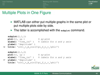
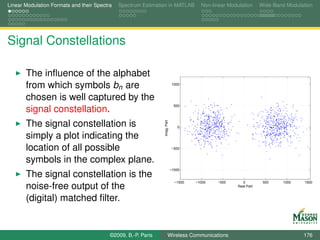
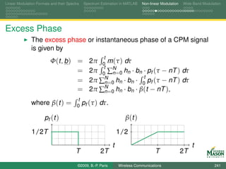
![User Interface Working with Vectors Visualization
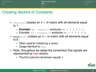
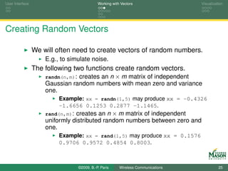
Commands for Creating Vectors
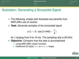
The following commands all create useful vectors.
[ ]: the sequence of samples is explicitly specified.
Example: xx = [ 1 3 2 ] produces xx = 1 3 2.
:(colon operator): creates a vector of equally spaced
samples.
Example: tt = 0:2:9 produces tt = 0 2 4 6 8.
Example: tt = 1:3 produces tt = 1 2 3.
Idiom: tt = ts:1/fs:te creates a vector of sampling times
between ts and te with sampling period 1/fs (i.e., the
sampling rate is fs).
©2009, B.-P. Paris Wireless Communications 23](https://image.slidesharecdn.com/handouts-122962284592-phpapp01/85/Simulation-of-Wireless-Communication-Systems-23-320.jpg)
![User Interface Working with Vectors Visualization
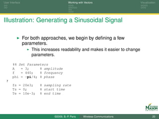
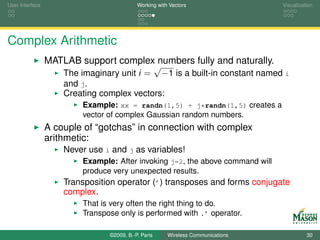
Addition and Subtraction
The standard + and - operators are used to add and
subtract vectors.
One of two conditions must hold for this operation to
succeed.
Both vectors must have exactly the same size.
In this case, corresponding elements in the two vectors are
added and the result is another vector of the same size.
Example: [1 3 2] + 1:3 produces 2 5 5.
A prominent error message indicates when this condition is
violated.
One of the operands is a scalar, i.e., a 1 × 1 (degenerate)
vector.
In this case, each element of the vector has the scalar added
to it.
The result is a vector of the same size as the vector operand.
Example: [1 3 2] + 2 produces 3 5 4.
©2009, B.-P. Paris Wireless Communications 26](https://image.slidesharecdn.com/handouts-122962284592-phpapp01/85/Simulation-of-Wireless-Communication-Systems-26-320.jpg)
![User Interface Working with Vectors Visualization
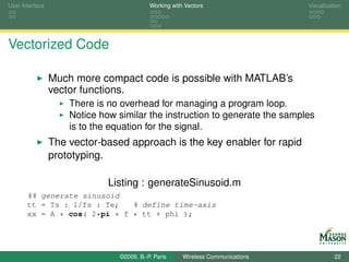
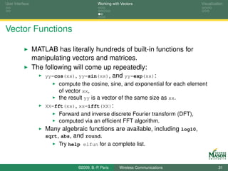
Element-wise Multiplication and Division
The operators .* and ./ operators multiply or divide two
vectors element by element.
One of two conditions must hold for this operation to
succeed.
Both vectors must have exactly the same size.
In this case, corresponding elements in the two vectors are
multiplied and the result is another vector of the same size.
Example: [1 3 2] .* 1:3 produces 1 6 6.
An error message indicates when this condition is violated.
One of the operands is a scalar.
In this case, each element of the vector is multiplied by the
scalar.
The result is a vector of the same size as the vector operand.
Example: [1 3 2] .* 2 produces 2 6 4.
If one operand is a scalar the ’.’ may be omitted, i.e.,
[1 3 2] * 2 also produces 2 6 4.
©2009, B.-P. Paris Wireless Communications 27](https://image.slidesharecdn.com/handouts-122962284592-phpapp01/85/Simulation-of-Wireless-Communication-Systems-27-320.jpg)
![User Interface Working with Vectors Visualization
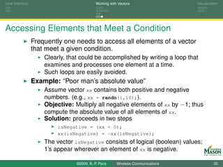
Inner Product
The operator * with two vector arguments computes the
inner product (dot product) of the vectors.
Recall the inner product of two vectors is defined as
N
x ·y = ∑ x (n ) · y (n ).
n =1
This implies that the result of the operation is a scalar!
The inner product is a useful and important signal
processing operation.
It is very different from element-wise multiplication.
The second dimension of the first operand must equal the
first dimension of the second operand.
MATLAB error message: Inner matrix dimensions
must agree.
Example: [1 3 2] * (1:3)’ = 13.
The single quote (’) transposes a vector.
©2009, B.-P. Paris Wireless Communications 28](https://image.slidesharecdn.com/handouts-122962284592-phpapp01/85/Simulation-of-Wireless-Communication-Systems-28-320.jpg)
![User Interface Working with Vectors Visualization
Powers
To raise a vector to some power use the .^ operator.
Example: [1 3 2].^2 yields 1 9 4.
The operator ^ exists but is generally not what you need.
Example: [1 3 2]^2 is equivalent to [1 3 2] * [1 3 2]
which produces an error.
Similarly, to use a vector as the exponent for a scalar base
use the .^ operator.
Example: 2.^[1 3 2] yields 2 8 4.
Finally, to raise a vector of bases to a vector of exponents
use the .^ operator.
Example: [1 3 2].^(1:3) yields 1 9 8.
The two vectors must have the same dimensions.
The .^ operator is (nearly) always the right operator.
©2009, B.-P. Paris Wireless Communications 29](https://image.slidesharecdn.com/handouts-122962284592-phpapp01/85/Simulation-of-Wireless-Communication-Systems-29-320.jpg)

![User Interface Working with Vectors Visualization
Accessing Elements of a Vector
Frequently it is necessary to modify or extract a subset of
the elements of a vector.
Accessing a single element of a vector:
Example: Let xx = [1 3 2], change the third element to 4.
Solution: xx(3) = 4; produces xx = 1 3 4.
Single elements are accessed by providing the index of the
element of interest in parentheses.
©2009, B.-P. Paris Wireless Communications 33](https://image.slidesharecdn.com/handouts-122962284592-phpapp01/85/Simulation-of-Wireless-Communication-Systems-33-320.jpg)
![User Interface Working with Vectors Visualization
Accessing Elements of a Vector
Accessing a range of elements of a vector:
Example: Let xx = ones(1,10);, change the first five
elements to −1.
Solution: xx(1:5) = -1*ones(1,5); Note, xx(1:5) = -1
works as well.
Example: Change every other element of xx to 2.
Solution: xx(2:2:end) = 2;;
Note that end may be use to denote the index of a vector’s
last element.
This is handy if the length of the vector is not known.
Example: Change third and seventh element to 3.
Solution: xx([3 7]) = 3;;
A set of elements of a vector is accessed by providing a
vector of indices in parentheses.
©2009, B.-P. Paris Wireless Communications 34](https://image.slidesharecdn.com/handouts-122962284592-phpapp01/85/Simulation-of-Wireless-Communication-Systems-34-320.jpg)
![User Interface Working with Vectors Visualization
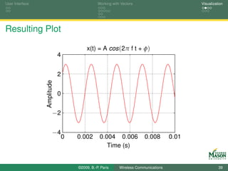
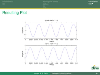
A Basic Plot
The sinusoidal signal, we generated earlier is easily plotted
via the following sequence of commands:
Try help plot for more information about the capabilities of
the plot command.
%% Plot
plot(tt, xx, ’r’) % xy-plot, specify red line
xlabel( ’Time (s)’ ) % labels for x and y axis
ylabel( ’Amplitude’ )
10 title( ’x(t) = A cos(2pi f t + phi)’)
grid % create a grid
axis([0 10e-3 -4 4]) % tweak the range for the axes
©2009, B.-P. Paris Wireless Communications 38](https://image.slidesharecdn.com/handouts-122962284592-phpapp01/85/Simulation-of-Wireless-Communication-Systems-38-320.jpg)

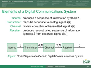
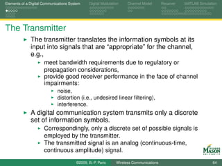
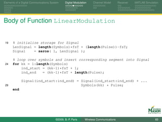
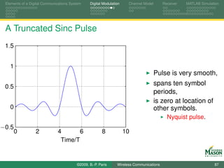
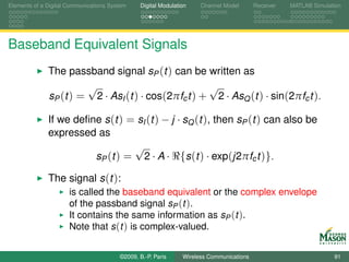
![Elements of a Digital Communications System Digital Modulation Channel Model Receiver MATLAB Simulation
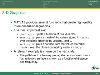
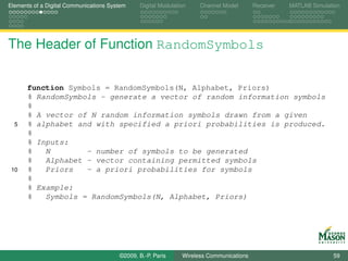
Modeling the Source in MATLAB
Objective: Write a MATLAB function to be invoked as:
Symbols = RandomSymbols( N, Alphabet, Priors);
The input parameters are
N: number of input symbols to be produced.
Alphabet: source alphabet to draw symbols from.
Example: Alphabet = [1 -1];
Priors: a priori probabilities for the input symbols.
Example:
Priors = ones(size(Alphabet))/length(Alphabet);
The output Symbols is a vector
with N elements,
drawn from Alphabet, and
the number of times each symbol occurs is (approximately)
proportional to the corresponding element in Priors.
©2009, B.-P. Paris Wireless Communications 55](https://image.slidesharecdn.com/handouts-122962284592-phpapp01/85/Simulation-of-Wireless-Communication-Systems-55-320.jpg)
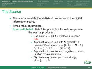
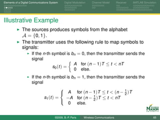
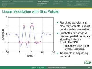
![Elements of a Digital Communications System Digital Modulation Channel Model Receiver MATLAB Simulation
Reminders
MATLAB’s basic data units are vectors and matrices.
Vectors are best thought of as lists of numbers; vectors
often contain samples of a signal.
There are many ways to create vectors, including
Explicitly: Alphabet = [1 -1];
Colon operator: nn = 1:10;
Via a function: Priors=ones(1,5)/5;
This leads to very concise programs; for-loops are rarely
needed.
MATLAB has a very large number of available functions.
Reduces programming to combining existing building
blocks.
Difficulty: find out what is available; use built-in help.
©2009, B.-P. Paris Wireless Communications 56](https://image.slidesharecdn.com/handouts-122962284592-phpapp01/85/Simulation-of-Wireless-Communication-Systems-56-320.jpg)
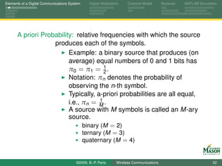
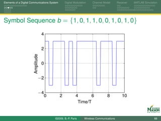
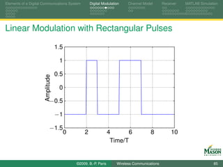
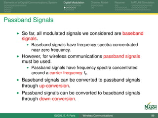
![Elements of a Digital Communications System Digital Modulation Channel Model Receiver MATLAB Simulation
Writing a MATLAB Function
A MATLAB function must
begin with a line of the form
function [out1,out2] = FunctionName(in1, in2, in3)
be stored in a file with the same name as the function name
and extension ’.m’.
For our symbol generator, the file name must be
RandomSymbols.m and
the first line must be
function Symbols = RandomSymbols(N, Alphabet, Priors)
©2009, B.-P. Paris Wireless Communications 57](https://image.slidesharecdn.com/handouts-122962284592-phpapp01/85/Simulation-of-Wireless-Communication-Systems-57-320.jpg)
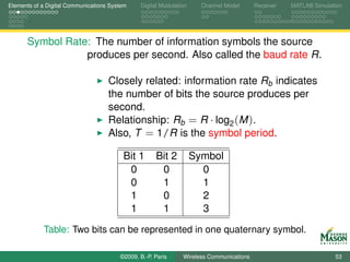
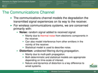
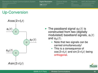
![Elements of a Digital Communications System Digital Modulation Channel Model Receiver MATLAB Simulation
Algorithm for Generating Random Symbols
For each of the symbols to be generated we use the
following algorithm:
Begin by computing the cumulative sum over the priors.
Example: Let Priors = [0.25 0.25 0.5], then the
cumulative sum equals CPriors = [0 0.25 0.5 1].
For each symbol, generate a uniform random number
between zero and one.
The MATLAB function rand does that.
Determine between which elements of the cumulative sum
the random number falls and select the corresponding
symbol from the alphabet.
Example: Assume the random number generated is 0.3.
This number falls between the second and third element of
CPriors.
The second symbol from the alphabet is selected.
©2009, B.-P. Paris Wireless Communications 60](https://image.slidesharecdn.com/handouts-122962284592-phpapp01/85/Simulation-of-Wireless-Communication-Systems-60-320.jpg)
![Elements of a Digital Communications System Digital Modulation Channel Model Receiver MATLAB Simulation
MATLAB Implementation
In MATLAB, the above algorithm can be “vectorized” to
work on the entire sequence at once.
CPriors = [0 cumsum( Priors )];
rr = rand(1, N);
for kk=1:length(Alphabet)
42 Matches = rr > CPriors(kk) & rr <= CPriors(kk+1);
Symbols( Matches ) = Alphabet( kk );
end
©2009, B.-P. Paris Wireless Communications 61](https://image.slidesharecdn.com/handouts-122962284592-phpapp01/85/Simulation-of-Wireless-Communication-Systems-61-320.jpg)
![Elements of a Digital Communications System Digital Modulation Channel Model Receiver MATLAB Simulation
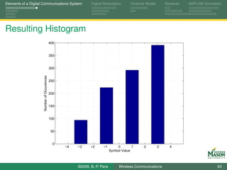
Testing Function RandomSymols
We can invoke and test the function RandomSymbols as
shown below.
A histogram of the generated symbols should reflect the
specified a priori probabilities.
%% set parameters
N = 1000;
Alphabet = [-3 -1 1 3];
Priors = [0.1 0.2 0.3 0.4];
10
%% generate symbols and plot histogram
Symbols = RandomSymbols( N, Alphabet, Priors );
hist(Symbols, -4:4 );
grid
15 xlabel(’Symbol Value’)
ylabel(’Number of Occurences’)
©2009, B.-P. Paris Wireless Communications 62](https://image.slidesharecdn.com/handouts-122962284592-phpapp01/85/Simulation-of-Wireless-Communication-Systems-62-320.jpg)
![Elements of a Digital Communications System Digital Modulation Channel Model Receiver MATLAB Simulation
MATLAB Code for Example
Listing : plot_TxExampleOrth.m
b = [ 1 0 1 1 0 0 1 0 1 0]; %symbol sequence
fsT = 20; % samples per symbol period
A = 3;
6
Signals = A*[ ones(1,fsT); % signals, one per row
ones(1,fsT/2) -ones(1,fsT/2)];
tt = 0:1/fsT:length(b)-1/fsT; % time axis for plotting
11
%% generate signal ...
TXSignal = [];
for kk=1:length(b)
TXSignal = [ TXSignal Signals( b(kk)+1, : ) ];
16 end
©2009, B.-P. Paris Wireless Communications 67](https://image.slidesharecdn.com/handouts-122962284592-phpapp01/85/Simulation-of-Wireless-Communication-Systems-67-320.jpg)
![Elements of a Digital Communications System Digital Modulation Channel Model Receiver MATLAB Simulation
MATLAB Code for Example
Listing : plot_TxExampleOrth.m
%% ... and plot
plot(tt, TXSignal)
20 axis([0 length(b) -(A+1) (A+1)]);
grid
xlabel(’Time/T’)
©2009, B.-P. Paris Wireless Communications 68](https://image.slidesharecdn.com/handouts-122962284592-phpapp01/85/Simulation-of-Wireless-Communication-Systems-68-320.jpg)
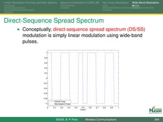
![Elements of a Digital Communications System Digital Modulation Channel Model Receiver MATLAB Simulation
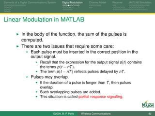
Testing Function LinearModulation
Listing : plot_LinearModRect.m
%% Parameters:
fsT = 20;
Alphabet = [1,-1];
6 Priors = 0.5*[1 1];
Pulse = ones(1,fsT); % rectangular pulse
%% symbols and Signal using our functions
Symbols = RandomSymbols(10, Alphabet, Priors);
11 Signal = LinearModulation(Symbols,Pulse,fsT);
%% plot
tt = (0 : length(Signal)-1 )/fsT;
plot(tt, Signal)
axis([0 length(Signal)/fsT -1.5 1.5])
16 grid
xlabel(’Time/T’)
ylabel(’Amplitude’)
©2009, B.-P. Paris Wireless Communications 84](https://image.slidesharecdn.com/handouts-122962284592-phpapp01/85/Simulation-of-Wireless-Communication-Systems-84-320.jpg)
![Elements of a Digital Communications System Digital Modulation Channel Model Receiver MATLAB Simulation
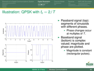
MATLAB Code for QPSK Illustration
Listing : plot_LinearModQPSK.m
%% Parameters:
fsT = 20;
L = 10;
fc = 2; % carrier frequency
7 Alphabet = [1, j, -j, -1];% QPSK
Priors = 0.25*[1 1 1 1];
Pulse = ones(1,fsT); % rectangular pulse
%% symbols and Signal using our functions
12 Symbols = RandomSymbols(10, Alphabet, Priors);
Signal = LinearModulation(Symbols,Pulse,fsT);
%% passband signal
tt = (0 : length(Signal)-1 )/fsT;
Signal_PB = sqrt(2)*real( Signal .* exp(-j*2*pi*fc*tt) );
©2009, B.-P. Paris Wireless Communications 93](https://image.slidesharecdn.com/handouts-122962284592-phpapp01/85/Simulation-of-Wireless-Communication-Systems-93-320.jpg)

![Elements of a Digital Communications System Digital Modulation Channel Model Receiver MATLAB Simulation
White Noise
The term white means specifically that
the mean of the noise is zero,
E[N (t )] = 0,
the autocorrelation function of the noise is
ρN (τ ) = E[N (t ) · N ∗ (t + τ )] = N0 δ(τ ).
This means that any distinct noise samples are
independent.
The autocorrelation function also indicates that noise
samples have infinite variance.
Insight: noise must be filtered before it can be sampled.
In-phase and quadrature noise each have autocorrelation
N0
2 δ ( τ ).
©2009, B.-P. Paris Wireless Communications 105](https://image.slidesharecdn.com/handouts-122962284592-phpapp01/85/Simulation-of-Wireless-Communication-Systems-105-320.jpg)

![Elements of a Digital Communications System Digital Modulation Channel Model Receiver MATLAB Simulation
Analog Front-end
Several, roughly equivalent, alternatives exist for the
analog front-end.
Two common approaches for the analog front-end will be
considered briefly.
Primarily, the analog front-end is responsible for converting
the continuous-time received signal R (t ) into a
discrete-time signal R [n].
Care must be taken with the conversion: (ideal) sampling
would admit too much noise.
Modeling the front-end faithfully is important for accurate
simulation.
©2009, B.-P. Paris Wireless Communications 118](https://image.slidesharecdn.com/handouts-122962284592-phpapp01/85/Simulation-of-Wireless-Communication-Systems-118-320.jpg)
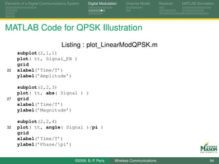
![Elements of a Digital Communications System Digital Modulation Channel Model Receiver MATLAB Simulation
Analog Front-end: Low-pass and Whitening Filter
The first structure contains
a low-pass filter (LPF) with bandwidth equal to the signal
bandwidth,
a sampler followed by a whitening filter (WF).
The low-pass filter creates correlated noise,
the whitening filter removes this correlation.
Sampler,
rate fs
R (t ) R [n] to
LPF WF
DSP
©2009, B.-P. Paris Wireless Communications 119](https://image.slidesharecdn.com/handouts-122962284592-phpapp01/85/Simulation-of-Wireless-Communication-Systems-119-320.jpg)
![Elements of a Digital Communications System Digital Modulation Channel Model Receiver MATLAB Simulation
Analog Front-end: Integrate-and-Dump
An alternative front-end has the structure shown below.
Here, ΠTs (t ) indicates a filter with an impulse response that
is a rectangular pulse of length Ts = 1/fs and amplitude
1/Ts .
The entire system is often called an integrate-and-dump
sampler.
Most analog-to-digital converters (ADC) operate like this.
A whitening filter is not required since noise samples are
uncorrelated.
Sampler,
rate fs
R (t ) R [n ] to
ΠTs (t )
DSP
©2009, B.-P. Paris Wireless Communications 120](https://image.slidesharecdn.com/handouts-122962284592-phpapp01/85/Simulation-of-Wireless-Communication-Systems-120-320.jpg)
![Elements of a Digital Communications System Digital Modulation Channel Model Receiver MATLAB Simulation
Output from Analog Front-end
The second of the analog front-ends is simpler
conceptually and widely used in practice;
it will be assumed for the remainder of the course.
For simulation purposes, we need to characterize the
output from the front-end.
To begin, assume that the received signal R (t ) consists of
a deterministic signal s (t ) and (AWGN) noise N (t ):
R (t ) = s (t ) + N (t ).
The signal R [n] is a discrete-time signal.
The front-end generates one sample every Ts seconds.
The discrete-time signal R [n] also consists of signal and
noise
R [n ] = s [n ] + N [n ].
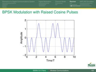
©2009, B.-P. Paris Wireless Communications 121](https://image.slidesharecdn.com/handouts-122962284592-phpapp01/85/Simulation-of-Wireless-Communication-Systems-121-320.jpg)
![Elements of a Digital Communications System Digital Modulation Channel Model Receiver MATLAB Simulation
Output from Analog Front-end
Consider the signal and noise component of the front-end
output separately.
This can be done because the front-end is linear.
The n-th sample of the signal component is given by:
1 (n+1)Ts
s [n ] = · s (t ) dt ≈ s ((n + 1/2)Ts ).
Ts nTs
The approximation is valid if fs = 1/Ts is much greater than
the signal band-width.
Sampler,
rate fs
R (t ) R [n ] to
ΠTs (t )
DSP
©2009, B.-P. Paris Wireless Communications 122](https://image.slidesharecdn.com/handouts-122962284592-phpapp01/85/Simulation-of-Wireless-Communication-Systems-122-320.jpg)
![Elements of a Digital Communications System Digital Modulation Channel Model Receiver MATLAB Simulation
Output from Analog Front-end
The noise samples N [n] at the output of the front-end:
are independent, complex Gaussian random variables, with
zero mean, and
variance equal to N0 /Ts .
The variance of the noise samples is proportional to 1/Ts .
Interpretations:
Noise is averaged over Ts seconds: variance decreases with
length of averager.
Bandwidth of front-end filter is approximately 1/Ts and
power of filtered noise is proportional to bandwidth (noise
bandwidth).
It will be convenient to express the noise variance as
N0 /T · T /Ts .
The factor T /Ts = fs T is the number of samples per
symbol period.
©2009, B.-P. Paris Wireless Communications 123](https://image.slidesharecdn.com/handouts-122962284592-phpapp01/85/Simulation-of-Wireless-Communication-Systems-123-320.jpg)
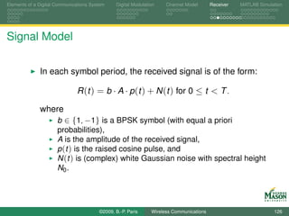
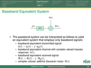
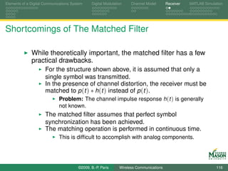
![Elements of a Digital Communications System Digital Modulation Channel Model Receiver MATLAB Simulation
System to be Simulated
Sampler,
N (t )
rate fs
bn s (t ) R (t ) R [n] to
× p (t ) × h (t ) + ΠTs (t )
DSP
∑ δ(t − nT ) A
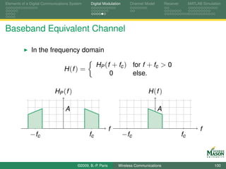
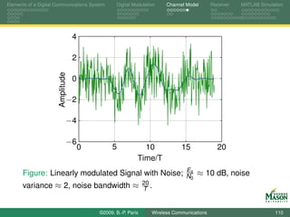
Figure: Baseband Equivalent System to be Simulated.
©2009, B.-P. Paris Wireless Communications 136](https://image.slidesharecdn.com/handouts-122962284592-phpapp01/85/Simulation-of-Wireless-Communication-Systems-136-320.jpg)
![Elements of a Digital Communications System Digital Modulation Channel Model Receiver MATLAB Simulation
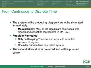
Towards the Discrete-Time Equivalent System
The shaded portion of the system has a discrete-time input
and a discrete-time output.
Can be considered as a discrete-time system.
Minor problem: input and output operate at different rates.
Sampler,
N (t )
rate fs
bn s (t ) R (t ) R [n] to
× p (t ) × h (t ) + ΠTs (t )
DSP
∑ δ(t − nT ) A
©2009, B.-P. Paris Wireless Communications 138](https://image.slidesharecdn.com/handouts-122962284592-phpapp01/85/Simulation-of-Wireless-Communication-Systems-138-320.jpg)
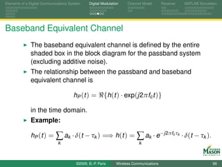
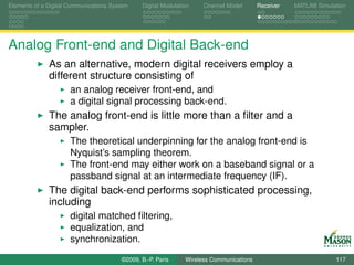
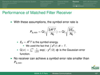
![Elements of a Digital Communications System Digital Modulation Channel Model Receiver MATLAB Simulation
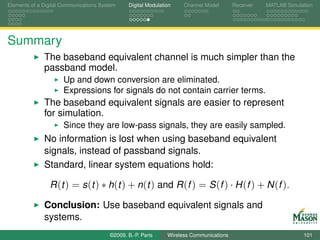
Discrete-Time Equivalent System
The discrete-time equivalent system
is equivalent to the original system, and
contains only discrete-time signals and components.
Input signal is up-sampled by factor fs T to make input and
output rates equal.
Insert fs T − 1 zeros between input samples.
N [n ]
bn R [n ]
× ↑ fs T h [n ] + to DSP
A
©2009, B.-P. Paris Wireless Communications 139](https://image.slidesharecdn.com/handouts-122962284592-phpapp01/85/Simulation-of-Wireless-Communication-Systems-139-320.jpg)
![Elements of a Digital Communications System Digital Modulation Channel Model Receiver MATLAB Simulation
Components of Discrete-Time Equivalent System
Question: What is the relationship between the
components of the original and discrete-time equivalent
system?
Sampler,
N (t )
rate fs
bn s (t ) R (t ) R [n] to
× p (t ) × h (t ) + ΠTs (t )
DSP
∑ δ(t − nT ) A
©2009, B.-P. Paris Wireless Communications 140](https://image.slidesharecdn.com/handouts-122962284592-phpapp01/85/Simulation-of-Wireless-Communication-Systems-140-320.jpg)
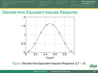
![Elements of a Digital Communications System Digital Modulation Channel Model Receiver MATLAB Simulation
Discrete-time Equivalent Impulse Response
To determine the impulse response h[n] of the
discrete-time equivalent system:
Set noise signal Nt to zero,
set input signal bn to unit impulse signal δ[n],
output signal is impulse response h[n].
Procedure yields:
1 ( n + 1 ) Ts
h [n ] = p (t ) ∗ h(t ) dt
Ts nTs
For high sampling rates (fs T 1), the impulse response is
closely approximated by sampling p (t ) ∗ h(t ):
h[n] ≈ p (t ) ∗ h(t )|(n+ 1 )Ts
2
©2009, B.-P. Paris Wireless Communications 141](https://image.slidesharecdn.com/handouts-122962284592-phpapp01/85/Simulation-of-Wireless-Communication-Systems-141-320.jpg)
![Elements of a Digital Communications System Digital Modulation Channel Model Receiver MATLAB Simulation
Discrete-Time Equivalent Noise
To determine the properties of the additive noise N [n] in
the discrete-time equivalent system,
Set input signal to zero,
let continuous-time noise be complex, white, Gaussian with
power spectral density N0 ,
output signal is discrete-time equivalent noise.
Procedure yields: The noise samples N [n]
are independent, complex Gaussian random variables, with
zero mean, and
variance equal to N0 /Ts .
©2009, B.-P. Paris Wireless Communications 143](https://image.slidesharecdn.com/handouts-122962284592-phpapp01/85/Simulation-of-Wireless-Communication-Systems-143-320.jpg)
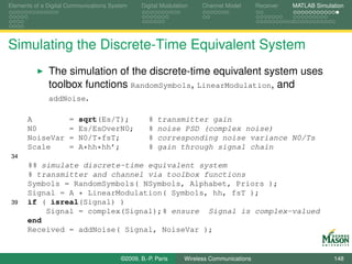
![Elements of a Digital Communications System Digital Modulation Channel Model Receiver MATLAB Simulation
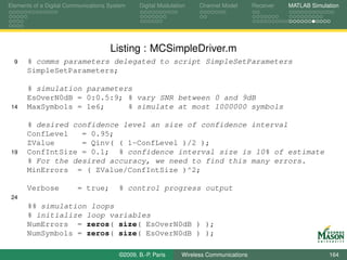
Listing : SimpleSetParameters.m
% This script sets a structure named Parameters to be used by
% the system simulator.
%% Parameters
7 % construct structure of parameters to be passed to system simulator
% communications parameters
Parameters.T = 1/10000; % symbol period
Parameters.fsT = 8; % samples per symbol
Parameters.Es = 1; % normalize received symbol energy to 1
12 Parameters.EsOverN0 = 6; % Signal-to-noise ratio (Es/N0)
Parameters.Alphabet = [1 -1]; % BPSK
Parameters.NSymbols = 1000; % number of Symbols
% discrete-time equivalent impulse response (raised cosine pulse)
17 fsT = Parameters.fsT;
tts = ( (0:fsT-1) + 1/2 )/fsT;
Parameters.hh = sqrt(2/3) * ( 1 - cos(2*pi*tts)*sin(pi/fsT)/(pi/fsT));
©2009, B.-P. Paris Wireless Communications 146](https://image.slidesharecdn.com/handouts-122962284592-phpapp01/85/Simulation-of-Wireless-Communication-Systems-146-320.jpg)
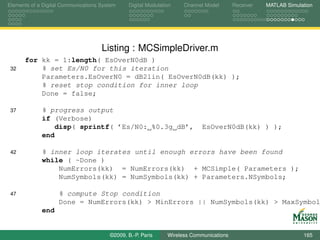
![Elements of a Digital Communications System Digital Modulation Channel Model Receiver MATLAB Simulation
Simulating the Discrete-Time Equivalent System
The actual system simulation is carried out in MATLAB
function MCSimple which has the function signature below.
The parameters set in the controlling script are passed as
inputs.
The body of the function simulates the transmission of the
signal and subsequent demodulation.
The number of incorrect decisions is determined and
returned.
function [NumErrors, ResultsStruct] = MCSimple( ParametersStruct )
©2009, B.-P. Paris Wireless Communications 147](https://image.slidesharecdn.com/handouts-122962284592-phpapp01/85/Simulation-of-Wireless-Communication-Systems-147-320.jpg)
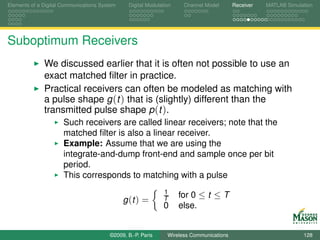
![Elements of a Digital Communications System Digital Modulation Channel Model Receiver MATLAB Simulation
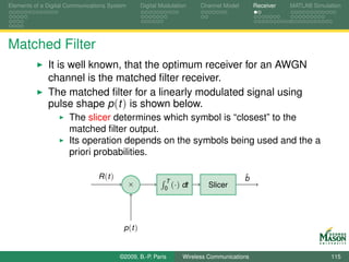
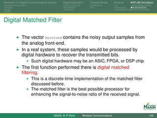
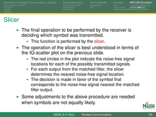
Digital Matched Filter
In our simulator, the vector Received is passed through a
discrete-time matched filter and down-sampled to the
symbol rate.
The impulse response of the matched filter is the conjugate
complex of the time-reversed, discrete-time channel
response h[n].
R [n ] ˆ
bn
h∗ [−n] ↓ fs T Slicer
©2009, B.-P. Paris Wireless Communications 150](https://image.slidesharecdn.com/handouts-122962284592-phpapp01/85/Simulation-of-Wireless-Communication-Systems-150-320.jpg)
![Elements of a Digital Communications System Digital Modulation Channel Model Receiver MATLAB Simulation
MATLAB Function SimpleSlicer
The procedure above is implemented in a function with
signature
function [Decisions, MSE] = SimpleSlicer( MFOut, Alphabet, Scale )
%% Loop over symbols to find symbol closest to MF output
for kk = 1:length( Alphabet )
% noise-free signal location
28 NoisefreeSig = Scale*Alphabet(kk);
% Euclidean distance between each observation and constellation po
Dist = abs( MFOut - NoisefreeSig );
% find locations for which distance is smaller than previous best
ChangedDec = ( Dist < MinDist );
33
% store new min distances and update decisions
MinDist( ChangedDec) = Dist( ChangedDec );
Decisions( ChangedDec ) = Alphabet(kk);
end
©2009, B.-P. Paris Wireless Communications 155](https://image.slidesharecdn.com/handouts-122962284592-phpapp01/85/Simulation-of-Wireless-Communication-Systems-155-320.jpg)
![Elements of a Digital Communications System Digital Modulation Channel Model Receiver MATLAB Simulation
Entire System
The addition of functions for the digital matched filter
completes the simulator for the communication system.
The functionality of the simulator is encapsulated in a
function with signature
function [NumErrors, ResultsStruct] = MCSimple( ParametersStruct )
The function simulates the transmission of a sequence of
symbols and determines how many symbol errors occurred.
The operation of the simulator is controlled via the
parameters passed in the input structure.
The body of the function is shown on the next slide; it
consists mainly of calls to functions in our toolbox.
©2009, B.-P. Paris Wireless Communications 156](https://image.slidesharecdn.com/handouts-122962284592-phpapp01/85/Simulation-of-Wireless-Communication-Systems-156-320.jpg)
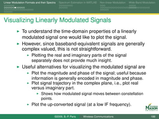

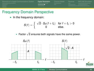
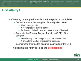
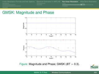
![Linear Modulation Formats and their Spectra Spectrum Estimation in MATLAB Non-linear Modulation Wide-Band Modulation
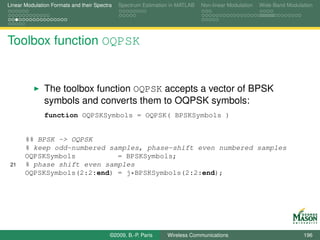
Toolbox function DPSK
The toolbox function DPSK with the following function
signature provides generic differential phase encoding:
1 function DPSKSymbols = DPSK( PAMSymbols, phi0, theta0 )
The body of DPSK computes differentially encoded
symbols as follows:
%% accumulate phase differences, then convert to complex symbols
Phases = cumsum( [theta0 phi0*PAMSymbols] );
DPSKSymbols = exp( j*Phases );
©2009, B.-P. Paris Wireless Communications 207](https://image.slidesharecdn.com/handouts-122962284592-phpapp01/85/Simulation-of-Wireless-Communication-Systems-207-320.jpg)
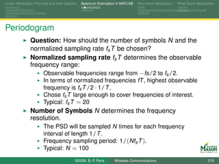
![Linear Modulation Formats and their Spectra Spectrum Estimation in MATLAB Non-linear Modulation Wide-Band Modulation
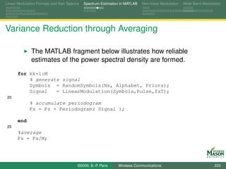
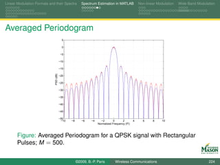
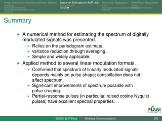
Improving the Periodogram Estimate
The periodogram estimate is extremely noisy.
ˆ
It is known that the periodogram Ps (f ) has a Gaussian
distribution and
ˆ
is an unbiased estimate E[Ps (f )] = Ps (f ),
ˆ
has variance Var[Ps (f )] = Ps (f ).
The variance of the periodogram is too high for the estimate
to be useful.
Fortunately, the variance is easily reduced through
averaging:
Generate M realizations of the modulated signal, and
average the periodograms for the signals.
Reduces variance by factor M.
©2009, B.-P. Paris Wireless Communications 222](https://image.slidesharecdn.com/handouts-122962284592-phpapp01/85/Simulation-of-Wireless-Communication-Systems-222-320.jpg)
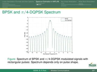
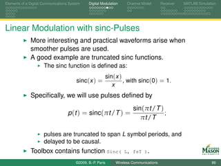
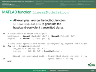
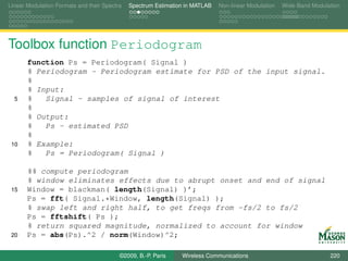
![Linear Modulation Formats and their Spectra Spectrum Estimation in MATLAB Non-linear Modulation Wide-Band Modulation
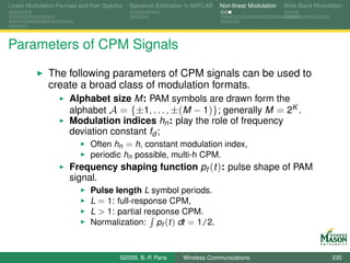
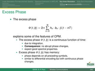
Generating CPM Signals in MATLAB
We have enough information to write a toolbox function to
generate CPM signal; it has the signature
function [CPMSignal, PAMSignal] = CPM(Symbols, A, h, Pulse, fsT)
The body of the function
calls LinearModulation to generate the PAM signal,
performs numerical integration through a suitable IIR filter
%% Generate PAM signal, using function LinearModulation
PAMSignal = LinearModulation( Symbols, Pulse, fsT );
%% Integrate PAM signal using a filter with difference equation
30 % y(n) = y(n-1) + x(n)/fsT and multiply with 2*pi*h
a = [1 -1];
b = 1/fsT;
Phase = 2*pi*h*filter(b, a, PAMSignal);
35 %% Baseband equivalent signal
CPMSignal = A*exp(j*Phase);
©2009, B.-P. Paris Wireless Communications 236](https://image.slidesharecdn.com/handouts-122962284592-phpapp01/85/Simulation-of-Wireless-Communication-Systems-236-320.jpg)
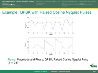
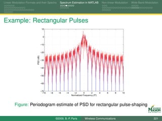
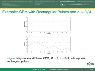
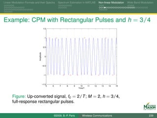
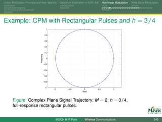
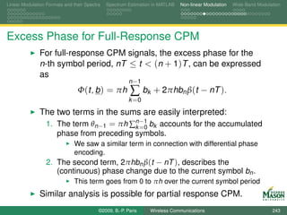
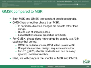
![Linear Modulation Formats and their Spectra Spectrum Estimation in MATLAB Non-linear Modulation Wide-Band Modulation
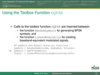
Using Toolbox Function CPM
A typical invocation of the function CPM is as follows:
%% Parameters:
fsT = 20;
Alphabet = [1,-1]; % 2-PAM
6 Priors = ones( size( Alphabet) ) / length(Alphabet);
Ns = 20; % number of symbols
Pulse = RectPulse( fsT); % Rectangular pulse
A = 1; % amplitude
h = 0.75; % modulation index
11
%% symbols and Signal using our functions
Symbols = RandomSymbols(Ns, Alphabet, Priors);
Signal = CPM(Symbols, A, h, Pulse,fsT);
©2009, B.-P. Paris Wireless Communications 237](https://image.slidesharecdn.com/handouts-122962284592-phpapp01/85/Simulation-of-Wireless-Communication-Systems-237-320.jpg)
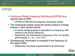
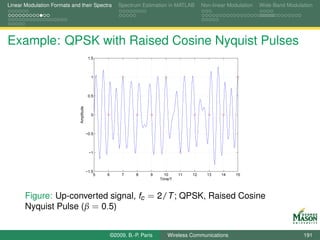
![Linear Modulation Formats and their Spectra Spectrum Estimation in MATLAB Non-linear Modulation Wide-Band Modulation
Digital Synthesis of a Carrier Modulated Signal
To start, assume we wanted to generate the samples for a
linearly modulated signal:
symbol for the m-th symbol period bm (k ),
N samples per symbol period,
rectangular pulses,
up-conversion to digital frequency k /N (physical frequency
fs · k /N).
The resulting samples in the m-th symbol period are
sm,k [n] = bm (k ) · exp(j2πkn/N ) for n = 0, 1, . . . , N − 1.
If these samples were passed through a D-to-A converter,
we would observe a signal spectrum
centered at frequency fs · k /N, and
bandwidth 2fs /N.
©2009, B.-P. Paris Wireless Communications 269](https://image.slidesharecdn.com/handouts-122962284592-phpapp01/85/Simulation-of-Wireless-Communication-Systems-269-320.jpg)
![Linear Modulation Formats and their Spectra Spectrum Estimation in MATLAB Non-linear Modulation Wide-Band Modulation
Combining Carriers
The single carrier occupies only a small fraction of the
bandwidth fs the A-to-D converter can process.
The remaining bandwidth can be used for additional
signals.
Specifically, we can combine N such signals.
Carrier frequencies: fs · k /N for k = 0, 1, . . . N − 1.
Resulting carriers are all orthogonal.
Samples of the combined signal in the m-th symbol period
are
N −1 N −1
sm [ n ] = ∑ sm,k [n] = ∑ bm (k ) · exp(j2πkn/N ).
k =0 k =0
The signal sm [n] represents N orthogonal narrow-band
signals multiplexed in the frequency domain (OFDM).
©2009, B.-P. Paris Wireless Communications 270](https://image.slidesharecdn.com/handouts-122962284592-phpapp01/85/Simulation-of-Wireless-Communication-Systems-270-320.jpg)
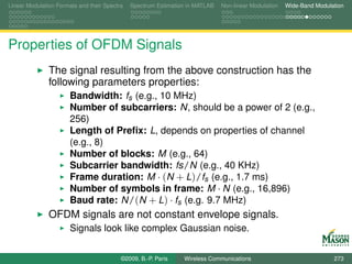
![Linear Modulation Formats and their Spectra Spectrum Estimation in MATLAB Non-linear Modulation Wide-Band Modulation
Constructing an OFDM Signal
The expression
N −1
sm [ n ] = ∑ bm (k ) · exp(j2πkn/N ).
k =0
represents the inverse DFT of the symbols bm (k ).
Direct evaluation of this equation requires N 2
multiplications and additions.
However, the structure of the expression permits
computationally efficient construction of sm [n] through an
FFT algorithm.
MATLAB’s function ifft can be used.
©2009, B.-P. Paris Wireless Communications 271](https://image.slidesharecdn.com/handouts-122962284592-phpapp01/85/Simulation-of-Wireless-Communication-Systems-271-320.jpg)
![Linear Modulation Formats and their Spectra Spectrum Estimation in MATLAB Non-linear Modulation Wide-Band Modulation
Constructing an OFDM Signal
The above considerations suggest the following procedure
for constructing an OFDM signal from a sequence of
information symbols b:
1. Serial-to-parallel conversion: break the sequence of
information symbols b into blocks of length N;
denote the k -th symbol in the m-th block as bm (k ).
2. Inverse DFT: Take the inverse FFT of each block m;
The output are length-N blocks of complex signal samples
denoted sm [n].
3. Cyclic prefix: Prepend the final L samples from each block
to the beginning of each block.
Cyclic protects against ISI.
4. Parallel-to-serial conversion: Concatenate the blocks to
form the OFDM signal.
©2009, B.-P. Paris Wireless Communications 272](https://image.slidesharecdn.com/handouts-122962284592-phpapp01/85/Simulation-of-Wireless-Communication-Systems-272-320.jpg)
![Linear Modulation Formats and their Spectra Spectrum Estimation in MATLAB Non-linear Modulation Wide-Band Modulation
Toolbox Function OFDMMod
%% Serial-to-parallel conversion
NBlocks = ceil( length(Symbols) / NCarriers );
% zero-pad, if needed
33 Blocks = zeros( 1, NBlocks*NCarriers );
Blocks(1:length(Symbols)) = Symbols;
% serial-to-parallel
Blocks = reshape( Blocks, NCarriers, NBlocks );
38 %% IFFT
% ifft works column-wise by default
Blocks = ifft( Blocks );
%% cyclic prefix
43 % copy last LPrefix samples of each column and prepend
Blocks = [ Blocks( end-LPrefix+1 : end, : ) ; Blocks ];
%% Parallel-to-serial conversion
Signal = reshape( Blocks, 1, NBlocks*(NCarriers+LPrefix) ) * ...
48 sqrt(NCarriers); % makes "gain" of ifft equal to 1.
©2009, B.-P. Paris Wireless Communications 275](https://image.slidesharecdn.com/handouts-122962284592-phpapp01/85/Simulation-of-Wireless-Communication-Systems-275-320.jpg)
![Linear Modulation Formats and their Spectra Spectrum Estimation in MATLAB Non-linear Modulation Wide-Band Modulation
Toolbox Function OFDMDemod
%% Serial-to-parallel conversion
32 NBlocks = ceil( length(Signal) / (NCarriers+LPrefix) );
if ( (NCarriers+LPrefix)*NBlocks ~= length(Signal) )
error(’Length of Signal must be a multiple of (NCarriers+LPrefix)’
end
% serial-to-parallel
37 Blocks = reshape( Signal/sqrt(NCarriers), NCarriers+LPrefix, NBlocks )
%% remove cyclic prefix
% remove first LPrefix samples of each column
Blocks( 1:LPrefix, : ) = [ ];
42
%% FFT
% fft works column-wise by default
Blocks = fft( Blocks );
47 %% Parallel-to-serial conversion
SymbolEst = reshape( Blocks, 1, NBlocks*NCarriers );
% remove zero-padding
SymbolEst = SymbolEst(1:NSymbols);
©2009, B.-P. Paris Wireless Communications 276](https://image.slidesharecdn.com/handouts-122962284592-phpapp01/85/Simulation-of-Wireless-Communication-Systems-276-320.jpg)

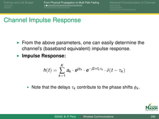

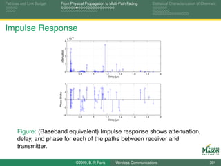
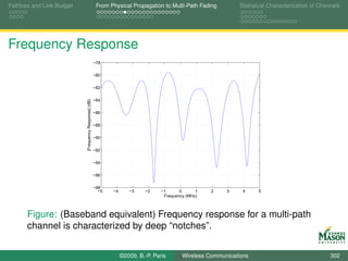
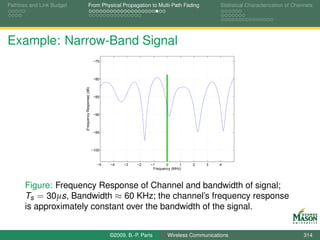
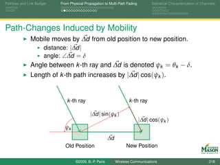
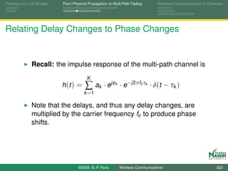
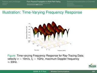
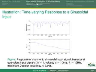
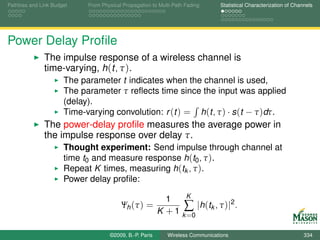
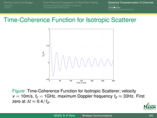
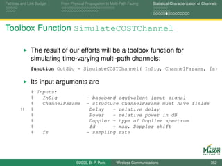
![Pathloss and Link Budget From Physical Propagation to Multi-Path Fading Statistical Characterization of Channels
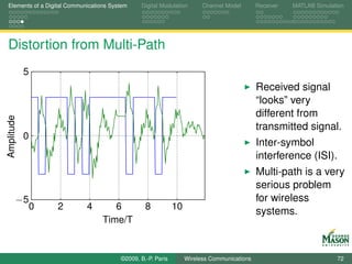
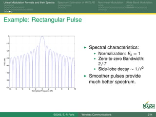
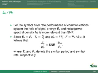
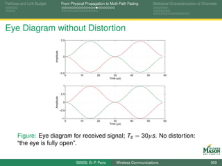
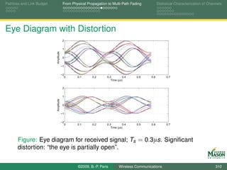
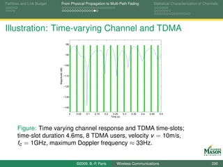
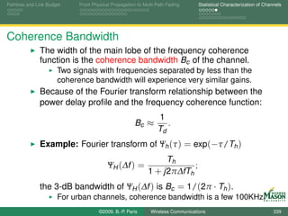
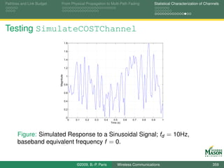
Eye Diagrams for Visualizing Distortion
An eye diagram is a simple but useful tool for quickly
gaining an appreciation for the amount of distortion present
in a received signal.
An eye diagram is obtained by plotting many segments of
the received signal on top of each other.
The segments span two symbol periods.
This can be accomplished in MATLAB via the command
plot( tt(1:2*fsT), real(reshape(Received(1:Ns*fsT), 2*fsT, [ ])))
Ns - number of symbols; should be large (e.g., 1000),
Received - vector of received samples.
The reshape command turns the vector into a matrix with
2*fsT rows, and
the plot command plots each column of the resulting matrix
individually.
©2009, B.-P. Paris Wireless Communications 308](https://image.slidesharecdn.com/handouts-122962284592-phpapp01/85/Simulation-of-Wireless-Communication-Systems-308-320.jpg)

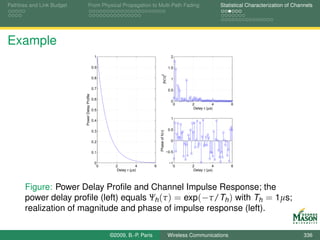
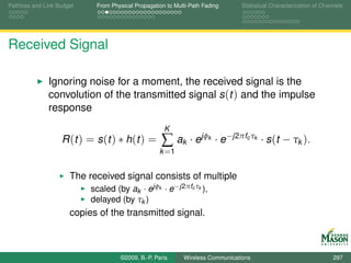
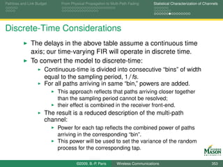
![Pathloss and Link Budget From Physical Propagation to Multi-Path Fading Statistical Characterization of Channels
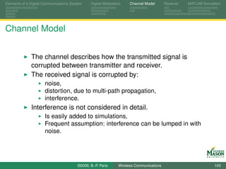
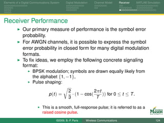
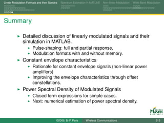
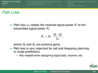
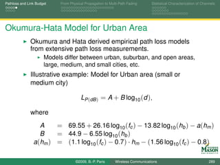
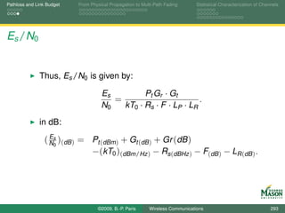
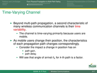
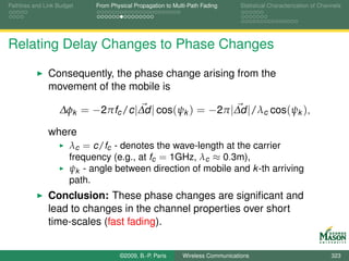
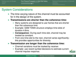
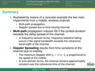
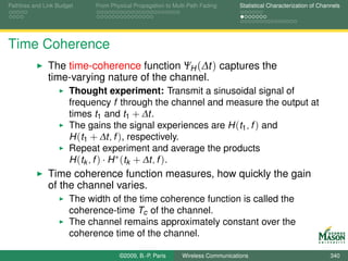
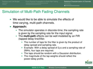
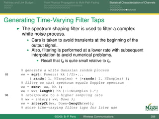
Simulation of Multi-Path Fading Channels
The taps are modeled as
Gaussian random processes
with variances given by the power delay profile, and
power spectral density given by the Doppler spectrum.
s [n ]
D D
a0 (t ) × a1 ( t ) × a2 (t ) ×
r [n ]
+ +
©2009, B.-P. Paris Wireless Communications 349](https://image.slidesharecdn.com/handouts-122962284592-phpapp01/85/Simulation-of-Wireless-Communication-Systems-349-320.jpg)
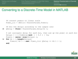


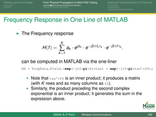
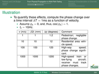
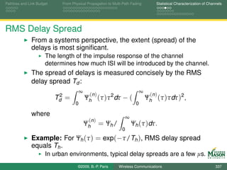
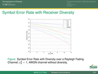
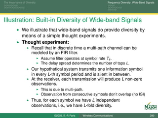
![The Importance of Diversity Frequency Diversity: Wide-Band Signals
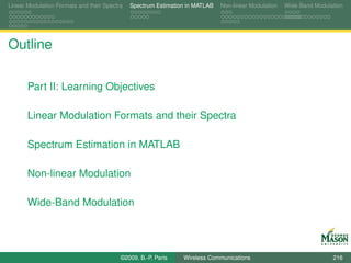
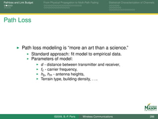
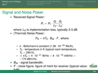
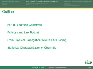
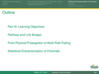
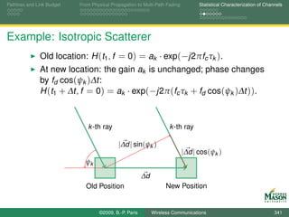
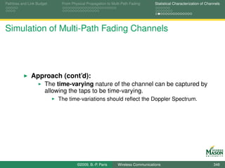
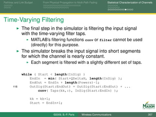
System to be Analyzed
The simple communication system in the diagram below
will be analyzed.
Focus on the effects of the multi-path channel h(t ).
Assumption: low baud rate, i.e., narrow-band signal.
Sampler,
N (t )
rate fs
bn s (t ) R (t ) R [n] to
× p (t ) × h (t ) + ΠTs (t )
DSP
∑ δ(t − nT ) A
©2009, B.-P. Paris Wireless Communications 368](https://image.slidesharecdn.com/handouts-122962284592-phpapp01/85/Simulation-of-Wireless-Communication-Systems-368-320.jpg)
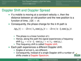
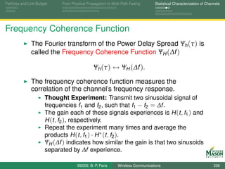
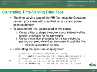
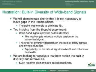
![The Importance of Diversity Frequency Diversity: Wide-Band Signals
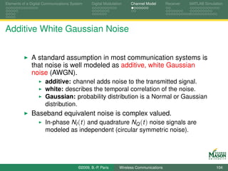
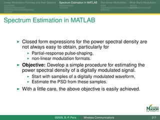
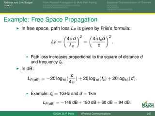
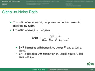
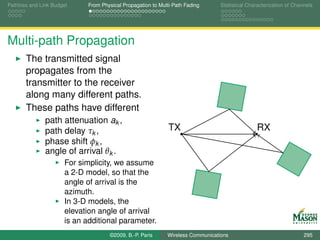
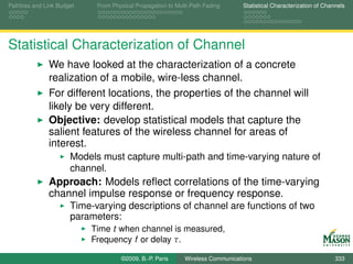
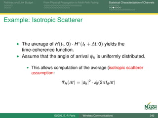
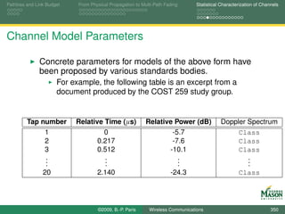
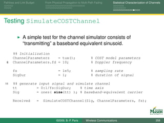
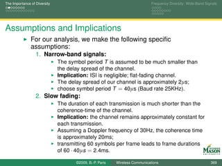
Implications on Channel Model
With the above assumptions, the multi-path channel
reduces effectively to attenuation by a factor a.
a is complex Gaussian (multiplicative noise),
The magnitude |a| is Rayleigh distributed (Rayleigh fading).
Short frame duration implies a is constant during a frame.
Sampler,
N (t )
rate fs
bn s (t ) R (t ) R [n] to
× p (t ) × × + ΠTs (t )
DSP
∑ δ(t − nT ) A a
©2009, B.-P. Paris Wireless Communications 370](https://image.slidesharecdn.com/handouts-122962284592-phpapp01/85/Simulation-of-Wireless-Communication-Systems-370-320.jpg)
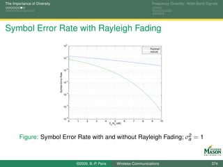
![The Importance of Diversity Frequency Diversity: Wide-Band Signals
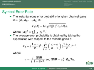
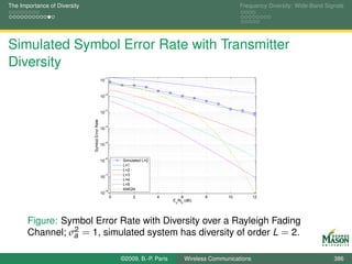
Average Symbol Error Rate
The instantaneous symbol error rate varies from frame to
frame and depends on a.
The average symbol error rate provides a measure of
performance that is independent of the attenuation a.
It is obtained by averaging over a:
Pe = E[Pe (a)] = Pe (a) · PA (a) da,
where PA (a) is the pdf for the attenuation a.
For a complex Gaussian attenuation a with zero mean and
2
variance σa :
1 SNR
Pe = (1 − ),
2 1 + SNR
2
where SNR = σa · Es /N0 .
©2009, B.-P. Paris Wireless Communications 373](https://image.slidesharecdn.com/handouts-122962284592-phpapp01/85/Simulation-of-Wireless-Communication-Systems-373-320.jpg)
![The Importance of Diversity Frequency Diversity: Wide-Band Signals
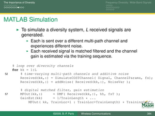
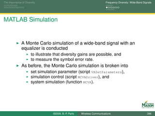
MATLAB Simulation
The simulation begins with the generation of the
transmitted signal.
New facet: a known training sequence is inserted in the
middle of the frame.
%% simulate discrete-time equivalent system
% transmitter and channel via toolbox functions
InfoSymbols = RandomSymbols( NSymbols, Alphabet, Priors );
% insert training sequence
45 Symbols = [ InfoSymbols(1:TrainLoc) TrainingSeq ...
InfoSymbols(TrainLoc+1:end)];
% linear modulation
©2009, B.-P. Paris Wireless Communications 383](https://image.slidesharecdn.com/handouts-122962284592-phpapp01/85/Simulation-of-Wireless-Communication-Systems-383-320.jpg)
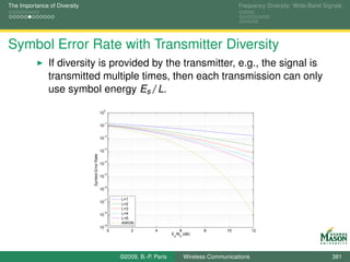
![The Importance of Diversity Frequency Diversity: Wide-Band Signals
MATLAB Simulation
The final processing step is maximum-ratio combining.
The matched filter outputs are multiplied with the conjugate
complex of the channel gains and added.
Multiplying with the conjugate complex of the channel gains
reverses phase rotations by the channel, and
gives more weight to strong channels.
61
% delete traning, MRC, and slicer
MFOut(:, TrainLoc+1 : TrainLoc+TrainLength) = [ ];
MRC = conj(GainEst)*MFOut;
Decisions = SimpleSlicer( MRC(1:NSymbols), Alphabet, ...
©2009, B.-P. Paris Wireless Communications 385](https://image.slidesharecdn.com/handouts-122962284592-phpapp01/85/Simulation-of-Wireless-Communication-Systems-385-320.jpg)


![The Importance of Diversity Frequency Diversity: Wide-Band Signals
Maximum Likelihood Sequence Estimation
The principle behind MLSE is simple.
Given a received sequence of samples R [n], e.g., matched
filter outputs, and
a model for the output of the multi-path channel:
r [n] = s [n] ∗ h[n], where
ˆ
s [n] denotes the symbol sequence, and
h[n] denotes the discrete-time channel impulse response,
i.e., the channel taps.
Find the sequence of information symbol s [n] that
minimizes
N
D2 = ∑ |r [n] − s[n] ∗ h[n]|2 .
n
©2009, B.-P. Paris Wireless Communications 394](https://image.slidesharecdn.com/handouts-122962284592-phpapp01/85/Simulation-of-Wireless-Communication-Systems-394-320.jpg)
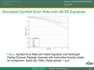
![The Importance of Diversity Frequency Diversity: Wide-Band Signals
Maximum Likelihood Sequence Estimation
The criterion
N
D2 = ∑ |r [n] − s[n] ∗ h[n]|2 .
n
performs diversity combining (via s [n] ∗ h[n]), and
removes ISI.
The minimization of the above metric is difficult because it
is a discrete optimization problem.
The symbols s [n] are from a discrete alphabet.
A computationally efficient algorithm exists to solve the
minimization problem:
The Viterbi Algorithm.
The toolbox contains an implementation of the Viterbi
Algorithm in function va.
©2009, B.-P. Paris Wireless Communications 395](https://image.slidesharecdn.com/handouts-122962284592-phpapp01/85/Simulation-of-Wireless-Communication-Systems-395-320.jpg)
![The Importance of Diversity Frequency Diversity: Wide-Band Signals
MATLAB Simulation: System Parameters
Listing : VASetParameters.m
Parameters.T = 1/1e6; % symbol period
Parameters.fsT = 8; % samples per symbol
Parameters.Es = 1; % normalize received symbol energy to 1
Parameters.EsOverN0 = 6; % Signal-to-noise ratio (Es/N0)
13 Parameters.Alphabet = [1 -1]; % BPSK
Parameters.NSymbols = 500; % number of Symbols per frame
Parameters.TrainLoc = floor(Parameters.NSymbols/2); % location of t
Parameters.TrainLength = 40;
18 Parameters.TrainingSeq = RandomSymbols( Parameters.TrainLength, ...
Parameters.Alphabet, [0.5 0.5]
% channel
Parameters.ChannelParams = tux(); % channel model
23 Parameters.fd = 3; % Doppler
Parameters.L = 6; % channel order
©2009, B.-P. Paris Wireless Communications 397](https://image.slidesharecdn.com/handouts-122962284592-phpapp01/85/Simulation-of-Wireless-Communication-Systems-397-320.jpg)
![The Importance of Diversity Frequency Diversity: Wide-Band Signals
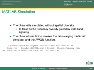
MATLAB Simulation
The first step in the system simulation is the simulation of
the transmitter functionality.
This is identical to the narrow-band case, except that the
baud rate is 1 MHz and 500 symbols are transmitted per
frame.
There are 40 training symbols.
Listing : MCVA.m
41 % transmitter and channel via toolbox functions
InfoSymbols = RandomSymbols( NSymbols, Alphabet, Priors );
% insert training sequence
Symbols = [ InfoSymbols(1:TrainLoc) TrainingSeq ...
InfoSymbols(TrainLoc+1:end)];
46 % linear modulation
Signal = A * LinearModulation( Symbols, hh, fsT );
©2009, B.-P. Paris Wireless Communications 398](https://image.slidesharecdn.com/handouts-122962284592-phpapp01/85/Simulation-of-Wireless-Communication-Systems-398-320.jpg)
![The Importance of Diversity Frequency Diversity: Wide-Band Signals
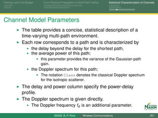
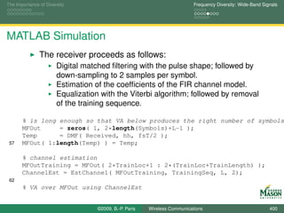
Channel Estimation
Channel Estimate:
h = (S S)−1 · S r,
ˆ
where
S is a Toeplitz matrix constructed from the training
sequence, and
r is the corresponding received signal.
TrainingSPS = zeros(1, length(Received) );
14 TrainingSPS(1:SpS:end) = Training;
% make into a Toepliz matrix, such that T*h is convolution
TrainMatrix = toeplitz( TrainingSPS, [Training(1) zeros(1, Order-1)]);
19 ChannelEst = Received * conj( TrainMatrix) * ...
inv(TrainMatrix’ * TrainMatrix);
©2009, B.-P. Paris Wireless Communications 401](https://image.slidesharecdn.com/handouts-122962284592-phpapp01/85/Simulation-of-Wireless-Communication-Systems-401-320.jpg)


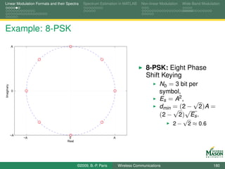
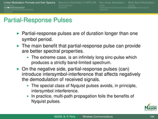
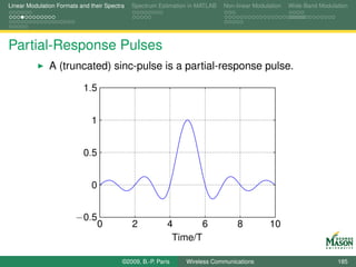
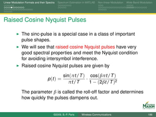
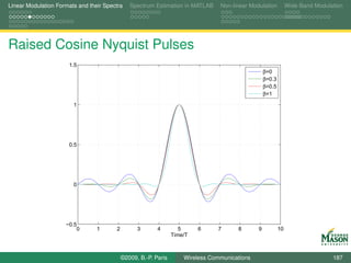
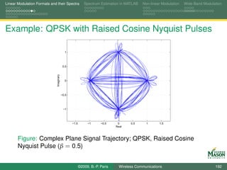
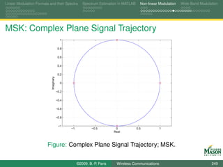
This document provides an outline for a course on modeling wireless communication systems using MATLAB. The course aims to cover both theoretical concepts and practical simulations. MATLAB will be used to illustrate key concepts and visualize signals. Students will learn the basics of MATLAB, including how to represent signals as vectors, perform vector operations, and use built-in functions to manipulate signals. Both theory and MATLAB simulations will be presented in parallel to make concepts concrete.