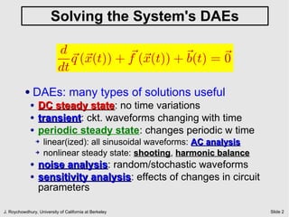
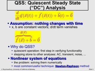
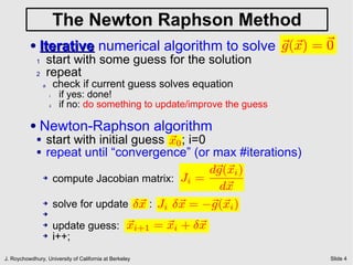
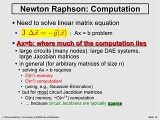
The document discusses quiescent steady state (DC) analysis using the Newton-Raphson method. It begins by introducing DC analysis and defining the goal as solving the system's differential algebraic equations (DAEs) under the assumption of no time variation. It then describes the Newton-Raphson method as an iterative numerical technique for solving nonlinear systems of equations. The method computes the Jacobian matrix at each iteration to determine the update to the state vector that will converge to a solution.

1. Quiescent Steady State (DC) Analysis
The Newton-Raphson Method
J. Roychowdhury, University of California at Berkeley Slide 1

2. Solving the System's DAEs
d
~ (~ (t)) + f (~ (t)) + ~ = ~
q x ~ x b(t) 0
dt
● DAEs: many types of solutions useful
● DC steady state: no time variations
state
● transient: ckt. waveforms changing with time
transient
● periodic steady state: changes periodic w time
➔ linear(ized): all sinusoidal waveforms: AC analysis
➔ nonlinear steady state: shooting, harmonic balance
shooting
● noise analysis: random/stochastic waveforms
analysis
● sensitivity analysis: effects of changes in circuit
analysis
parameters
J. Roychowdhury, University of California at Berkeley Slide 2

3. QSS: Quiescent Steady State
(“DC”) Analysis
d
~ (~ (t)) + f (~ (t)) + ~ = ~
q x ~ x b(t) 0
dt
● Assumption: nothing changes with time
● x, b are constant vectors; d/dt term vanishes
~ (~ )
g x
z }| {
f (~ ) + ~ = ~
~ x b 0
● Why do QSS?
➔ quiescent operation: first step in verifying functionality
➔ stepping stone to other analyses: AC, transient, noise, ...
● Nonlinear system of equations
➔ the problem: solving them numerically
➔ most common/useful technique: Newton-Raphson method
J. Roychowdhury, University of California at Berkeley Slide 3

4. The Newton Raphson Method
● Iterative numerical algorithm to solve ~ (~ ) = ~
g x 0
1 start with some guess for the solution
2 repeat
a check if current guess solves equation
i if yes: done!
ii if no: do something to update/improve the guess
● Newton-Raphson algorithm
● start with initial guess ~ 0 ; i=0
x
● repeat until “convergence” (or max #iterations)
d~ (~ i )
g x
➔ compute Jacobian matrix: Ji =
d~x
➔ solve for update ±~ : Ji ±~ = ¡~ (~ i )
x x g x
➔
➔ update guess: ~ i+1 = ~ i + ±~
x x x
➔ i++;
J. Roychowdhury, University of California at Berkeley Slide 4

5. Newton-Raphson Graphically
g(x)
● Scalar case above
● Key property: generalizes to vector case
J. Roychowdhury, University of California at Berkeley Slide 5

6. Newton Raphson (contd.)
● Does it always work? No.
● Conditions for NR to converge reliably
➔ g(x) must be “smooth”: continuous, differentiable
➔ starting guess “close enough” to solution
● practical NR: needs application-specific heuristics
J. Roychowdhury, University of California at Berkeley Slide 6

7. NR: Convergence Rate
● Key property of NR: quadratic convergence
¤
● Suppose x is the exact solution of g(x) = 0
● At the i
th
NR iteration, define the error ²i = xi ¡ x¤
● meaning of quadratic convergence: ²i+1 < c²2
i
●
(where c is a constant)
● NR's quadratic convergence properties
➔
if g(x) is smooth (at least continuous 1st and 2nd derivatives)
➔ and g 0 (x¤ ) 6= 0
➔ and kxi ¡ x¤ k is small enough, then:
➔ NR features quadratic convergence
J. Roychowdhury, University of California at Berkeley Slide 7

8. Convergence Rate in Digits of
Accuracy
Quadratic convergence Linear convergence
J. Roychowdhury, University of California at Berkeley Slide 8

9. NR: Convergence Strategies
● reltol-abstol on deltax
● stop if norm(deltax) <= tolerance
➔ tolerance = abstol + reltol*x
●
reltol ~ 1e-3 to 1e-6
●
abstol ~ 1e-9 to 1e-12
● better
➔ apply to individual vector entries (and AND)
➔ organize x in variable groups: e.g., voltages, currents, …
➔ (scale DAE equations/unknowns first)
● more sophisticated possible
➔ e.g., use sequence of x values to estimate conv. rate
● residual convergence criterion
● stop if k~ (~ )k < ²residual
g x
● Combinations of deltax and residual
● ultimately: heuristics, tuned to application
J. Roychowdhury, University of California at Berkeley Slide 9

10. Newton Raphson Update Step
● Need to solve linear matrix equation
● J ¢~ = ¡~ (~ ) : Ax = b problem
x g x
d~ (~ )
g x
● J= : Jacobian matrix
d~x
● Derivatives of vector functions
2 3 2 3
x1 g1 (x1 ; ¢ ¢ ¢ ; xn )
6 . 7 6 7
● If ~ (t) = 4 . 5 ;
x . ~ (~ ) = 4
g x .
.
. 5
xn g1 (x1 ; ¢ ¢ ¢ ; xn )
2 dg1 dg1 dg1 dg1
3
dx1 dx2 ¢¢¢ dxn¡1 dxn
6 dg2 dg2 dg2 dg2 7
6 ¢¢¢ 7
d~
g 6 dx1 dx2 dxn¡1 dxn 7
6 . . . . 7
● … then ,6 . . ¢¢¢ . . 7
x 6 dg .
d~ . . . 7
6 n¡1 dgn¡1
¢¢¢ dgn¡1 dgn¡1 7
4 dx1 dx2 dxn¡1 dxn 5
dgn dgn dgn dgn
dx1 dx2 ¢¢¢ dxn¡1 dxn
J. Roychowdhury, University of California at Berkeley Slide 10

11. DAE Jacobian Matrices
1
° 2
°
d
● Ckt DAE: ~ (~ (t)) + f (~ (t)) + ~ = ~
q x ~ x b(t) 0 iE
dt iL
2 3 2 2 3 3 2 3
e1 (t) 0 ¡diode(¡e1 ; IS ; Vt ) ¡ iE 0
6 e2 (t) 7 6 Ce2 7 6 0 7
~ (t) = 6 7 ~(~ ) = 6 7 f (~ ) = 6 iE + iL + e2 7~
7 b(t) = 6 7
x 4 iL (t) 5 q x 4 0 5 ~x 6
4 e2 ¡ e1
R
5 4¡E(t)5
iE (t) ¡LiL e2 0
2 3 2 ddiode 3
0 0 0 0 dv (¡e1 ) 0 0 ¡1
d~
q 60 C 0 07 ~ 6
df 0 1
1 17
Jq , =6
40
7 Jf , =6 R 7
d~
x 0 0 05 d~
x 4 ¡1 1 0 05
0 0 ¡L 0 0 1 0 0
J. Roychowdhury, University of California at Berkeley Slide 11

12. Newton Raphson: Computation
● Need to solve linear matrix equation
● J ¢~ = ¡~ (~ ) : Ax = b problem
x g x
● Ax=b: where much of the computation lies
● large circuits (many nodes): large DAE systems,
large Jacobian matrices
● in general (for arbitrary matrices of size n)
➔ solving Ax = b requires
●
O(n2) memory
●
O(n3) computation!
●
(using, e.g., Gaussian Elimination)
➔ but for most circuit Jacobian matrices
●
O(n) memory, ~O(n1.4) computation
●
… because circuit Jacobians are typically sparse
J. Roychowdhury, University of California at Berkeley Slide 12

13. Dense vs Sparse Matrices
● Sparse Jacobians: typically 3N-4N non-zeros
● compare against N2 for dense
J. Roychowdhury, University of California at Berkeley Slide 13