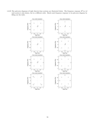
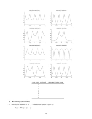
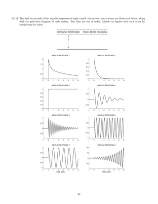
This document contains lecture notes on signals, systems and transforms for a course titled EE 3054: Signals, Systems and Transforms. It covers topics in discrete-time and continuous-time signals and systems, including properties of signals and systems, convolution, Z-transforms, Laplace transforms, difference/differential equations, complex poles, frequency responses, Fourier transforms, and sampling theory. The document provides examples and homework problems for students to work through related to each major topic.

1. EE 3054: Signals, Systems and Transforms
Exercises
Ivan W. Selesnick
March 25, 2013
Contents
1 Discrete-Time Signals and Systems 3
1.1 Signals . . . . . . . . . . . . . . . . . . . . . . . . . . . . . . . . . . . . . . . . . . . . . . . . . . . . . . 3
1.2 System Properties . . . . . . . . . . . . . . . . . . . . . . . . . . . . . . . . . . . . . . . . . . . . . . . 4
1.3 More Convolution . . . . . . . . . . . . . . . . . . . . . . . . . . . . . . . . . . . . . . . . . . . . . . . 9
1.4 Z Transforms . . . . . . . . . . . . . . . . . . . . . . . . . . . . . . . . . . . . . . . . . . . . . . . . . . 12
1.5 Inverse Systems . . . . . . . . . . . . . . . . . . . . . . . . . . . . . . . . . . . . . . . . . . . . . . . . . 16
1.6 Difference Equations . . . . . . . . . . . . . . . . . . . . . . . . . . . . . . . . . . . . . . . . . . . . . . 16
1.7 Complex Poles . . . . . . . . . . . . . . . . . . . . . . . . . . . . . . . . . . . . . . . . . . . . . . . . . 20
1.8 Frequency Responses . . . . . . . . . . . . . . . . . . . . . . . . . . . . . . . . . . . . . . . . . . . . . . 31
1.9 Summary Problems . . . . . . . . . . . . . . . . . . . . . . . . . . . . . . . . . . . . . . . . . . . . . . . 56
1.10 Simple System Design . . . . . . . . . . . . . . . . . . . . . . . . . . . . . . . . . . . . . . . . . . . . . 59
1.11 Matching . . . . . . . . . . . . . . . . . . . . . . . . . . . . . . . . . . . . . . . . . . . . . . . . . . . . 61
1.12 More Problems . . . . . . . . . . . . . . . . . . . . . . . . . . . . . . . . . . . . . . . . . . . . . . . . . 70
2 Continuous-Time Signals and Systems 73
2.1 Signals . . . . . . . . . . . . . . . . . . . . . . . . . . . . . . . . . . . . . . . . . . . . . . . . . . . . . . 73
2.2 System Properties . . . . . . . . . . . . . . . . . . . . . . . . . . . . . . . . . . . . . . . . . . . . . . . 74
2.3 Convolution . . . . . . . . . . . . . . . . . . . . . . . . . . . . . . . . . . . . . . . . . . . . . . . . . . . 80
2.4 Laplace Transform . . . . . . . . . . . . . . . . . . . . . . . . . . . . . . . . . . . . . . . . . . . . . . . 85
2.5 Differential Equations . . . . . . . . . . . . . . . . . . . . . . . . . . . . . . . . . . . . . . . . . . . . . 86
2.6 Complex Poles . . . . . . . . . . . . . . . . . . . . . . . . . . . . . . . . . . . . . . . . . . . . . . . . . 89
2.7 Frequency Response . . . . . . . . . . . . . . . . . . . . . . . . . . . . . . . . . . . . . . . . . . . . . . 97
2.8 Matching . . . . . . . . . . . . . . . . . . . . . . . . . . . . . . . . . . . . . . . . . . . . . . . . . . . . 124
2.9 Simple System Design . . . . . . . . . . . . . . . . . . . . . . . . . . . . . . . . . . . . . . . . . . . . . 125
2.10 Summary . . . . . . . . . . . . . . . . . . . . . . . . . . . . . . . . . . . . . . . . . . . . . . . . . . . . 127
2.11 Old Unused Problems . . . . . . . . . . . . . . . . . . . . . . . . . . . . . . . . . . . . . . . . . . . . . 134
3 Fourier Transform 136
3.1 Fourier Transform . . . . . . . . . . . . . . . . . . . . . . . . . . . . . . . . . . . . . . . . . . . . . . . 136
3.2 Fourier Series . . . . . . . . . . . . . . . . . . . . . . . . . . . . . . . . . . . . . . . . . . . . . . . . . . 144
3.3 Modulation . . . . . . . . . . . . . . . . . . . . . . . . . . . . . . . . . . . . . . . . . . . . . . . . . . . 146
4 The Sampling Theorem 148
1

2. HW 1
Signals: 1.1.1(a,b,c,d,g), 1.1.2, 1.1.6
System properties: 1.2.1 (a,b,c,d), 1.2.2, 1.2.4, 1.2.6, 1.2.7, 1.2.8
HW 2
Systems: 1.2.15, 1.2.17
Convolution: 1.3.1 (a, b, d, f), 1.3.2, 1.3.3, 1.3.7
Z-transforms: 1.4.1, 1.4.2, 1.4.3, 1.4.5, 1.4.7, 1.4.8, 1.4.9, 1.4.13
HW 3
Z-transforms: 1.4.15,
Inverse systems: 1.5.1, 1.5.2,
Difference equations: 1.6.1, 1.6.2, 1.6.3, 1.6.4, 1.6.5, 1.6.6, 1.6.7ab, 1.6.8, 1.6.13
HW 4
Difference equations: 1.6.9, 1.6.14,
Complex poles: 1.7.1 1.7.2, 1.7.3, 1.7.4, 1.7.7, 1.7.9, 1.7.10, 1.7.11, 1.7.12
HW 5
Frequency response: 1.8.1, 1.8.2, 1.8.3, 1.8.4, 1.8.5, 1.8.8, 1.8.9, 1.8.10, 1.8.12, 1.8.15, 1.8.16, 1.8.18, 1.8.22
HW 6
Frequency response: 1.8.24,
Summary exercises: 1.9.3, 1.9.8, 1.9.12,
Simple system design: 1.10.1, 1.10.3, 1.10.4,
Matching: 1.11.1,
More: 1.12.4
HW 7
Complex poles (discrete-time): 1.7.5,
Signals: 2.1.1, 2.1.2 (a,b,c,e),
System properties: 2.2.1, 2.2.3, 2.2.4, 2.2.5, 2.2.8, 2.2.13, 2.2.18
HW 8
System properties: 2.2.7, 2.2.11, 2.2.22,
Convolution: 2.3.1, 2.3.3, 2.3.4, 2.3.7, 2.3.10, 2.3.11, 2.3.12, 2.3.9,
HW 9
Convolution: 2.3.6, 2.3.14, 2.3.16, 2.3.17 (a,b,e),
Laplace transform: 2.4.1, 2.4.2, 2.4.3, 2.4.4, 2.4.5, 2.4.6,
Differential equations: 2.5.1, 2.5.2, 2.5.3, 2.5.4, 2.5.5, 2.5.12, 2.5.14
HW 10
Complex poles: 2.6.1, 2.6.2, 2.6.3, 2.6.4, 2.6.6, 2.6.10,
Frequency responses: 2.7.1, 2.7.2, 2.7.3, 2.7.5, 2.7.6, 2.7.7, 2.7.9, 2.7.17, 2.7.21, 2.7.23, 2.7.24, 2.7.29
HW 11
Systems: 2.9.2, 2.9.3
Fourier Transforms: 3.1.1a, 3.1.2, 3.1.3, 3.1.5, 3.1.7, 3.1.12, 3.1.14, 3.1.21, 3.1.22
Fourier Series: 3.2.1, 3.2.2, 3.2.3, 3.2.8,
HW 12
Sampling theorem:
2

3. 1 Discrete-Time Signals and Systems
1.1 Signals
1.1.1 Make an accurate sketch of each of the discrete-time signals
(a)
x(n) = u(n + 3) + 0.5 u(n − 1)
(b)
x(n) = δ(n + 3) + 0.5 δ(n − 1)
(c)
x(n) = 2n
· δ(n − 4)
(d)
x(n) = 2n
· u(−n − 2)
(e)
x(n) = (−1)n
u(−n − 4).
(f)
x(n) = 2 δ(n + 4) − δ(n − 2) + u(n − 3)
(g)
x(n) =
∞
k=0
4 δ(n − 3 k − 1)
(h)
x(n) =
∞
k=−∞
(−1)k
δ(n − 3 k)
1.1.2 Make a sketch of each of the following signals
(a)
x(n) =
∞
k=−∞
(0.9)
|k|
δ(n − k)
(b)
x(n) = cos(π n) u(n)
(c)
x(n) = u(n) − 2 u(n − 4) + u(n − 8)
1.1.3 Sketch x(n), x1(n), x2(n), and x3(n) where
x(n) = u(n + 4) − u(n), x1(n) = x(n − 3),
x2(n) = x(5 − n), x3(n) =
n
k=−∞
x(k)
3

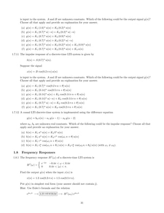
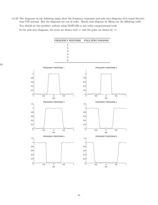
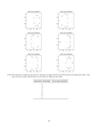
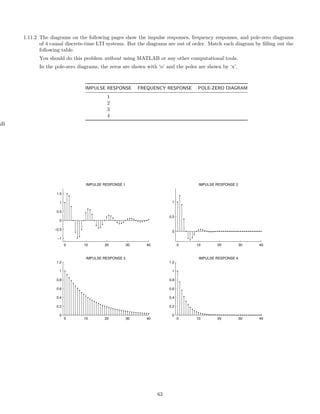
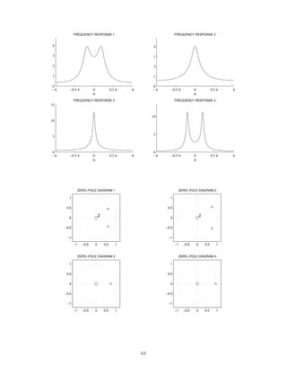
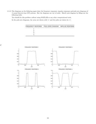
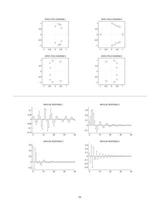
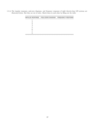
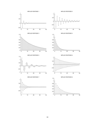
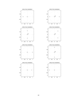
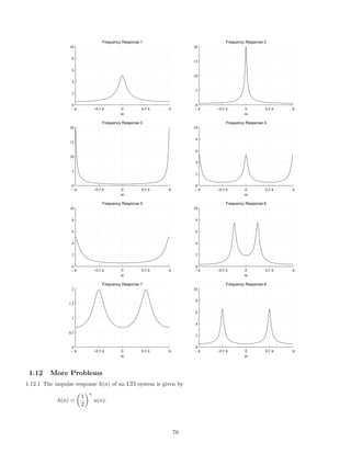
4. 1.1.4 Sketch x(n) and x1(n) where
x(n) = (0.5)n
u(n), x1(n) =
n
k=−∞
x(k)
1.1.5 Sketch x(n) and x1(n) where
x(n) = n [δ(n − 5) + δ(n − 3)], x1(n) =
n
k=−∞
x(k)
1.1.6 Make a sketch of each of the following signals
(a)
f(n) =
∞
k=0
(−0.9)
k
δ(n − 3 k)
(b)
g(n) =
∞
k=−∞
(−0.9)
|k|
δ(n − 3 k)
(c)
x(n) = cos(0.25 π n) u(n)
(d)
x(n) = cos(0.5 π n) u(n)
1.2 System Properties
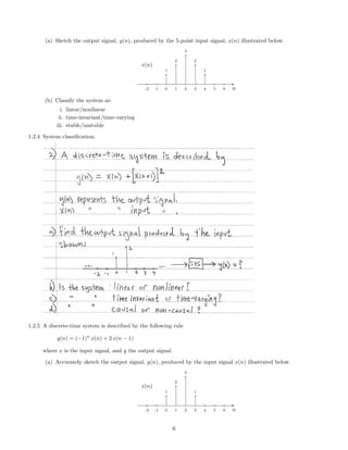
1.2.1 A discrete-time system may be classified as follows:
• memoryless/with memory
• causal/noncausal
• linear/nonlinear
• time-invariant/time-varying
• BIBO stable/unstable
Classify each of the following discrete-times systems.
(a)
y(n) = cos(x(n)).
(b)
y(n) = 2 n2
x(n) + n x(n + 1).
(c)
y(n) = max {x(n), x(n + 1)}
Note: the notation max{a, b} means for example; max{4, 6} = 6.
4

5. (d)
y(n) =
x(n) when n is even
x(n − 1) when n is odd
(e)
y(n) = x(n) + 2 x(n − 1) − 3 x(n − 2).
(f)
y(n) =
∞
k=0
(1/2)k
x(n − k).
That is,
y(n) = x(n) + (1/2) x(n − 1) + (1/4) x(n − 2) + · · ·
(g)
y(n) = x(2 n)
1.2.2 A discrete-time system is described by the following rule
y(n) = 0.5 x(2n) + 0.5 x(2n − 1)
where x is the input signal, and y the output signal.
(a) Sketch the output signal, y(n), produced by the 4-point input signal, x(n) illustrated below.
2
3
2
1
-2 -1 0 1 2 3 4 5 6 n
x(n)
(b) Sketch the output signal, y(n), produced by the 4-point input signal, x(n) illustrated below.
2
3
2
1
-2 -1 0 1 2 3 4 5 6 n
x(n)
(c) Classify the system as:
i. causal/non-causal
ii. linear/nonlinear
iii. time-invariant/time-varying
1.2.3 A discrete-time system is described by the following rule
y(n) =
x(n), when n is an even integer
−x(n), when n is an odd integer
where x is the input signal, and y the output signal.
5

6. (a) Sketch the output signal, y(n), produced by the 5-point input signal, x(n) illustrated below.
1
2
3
2
1
-2 -1 0 1 2 3 4 5 6 n
x(n)
(b) Classify the system as:
i. linear/nonlinear
ii. time-invariant/time-varying
iii. stable/unstable
1.2.4 System classification:
1.2.5 A discrete-time system is described by the following rule
y(n) = (−1)n
x(n) + 2 x(n − 1)
where x is the input signal, and y the output signal.
(a) Accurately sketch the output signal, y(n), produced by the input signal x(n) illustrated below.
1
2
3
1
-2 -1 0 1 2 3 4 5 6 n
x(n)
6

7. (b) Classify the system as:
i. causal/non-causal
ii. linear/nonlinear
iii. time-invariant/time-varying
1.2.6 Predict the output of an LTI system:
1.2.7 The impulse response of a discrete-time LTI system is
h(n) = 2 δ(n) + 3 δ(n − 1) + δ(n − 2).
Find and sketch the output of this system when the input is the signal
x(n) = δ(n) + 3 δ(n − 1) + 2 δ(n − 2).
1.2.8 Consider a discrete-time LTI system described by the rule
y(n) = x(n − 5) +
1
2
x(n − 7).
What is the impulse response h(n) of this system?
1.2.9 The impulse response of a discrete-time LTI system is
h(n) = δ(n) + 2 δ(n − 1) + δ(n − 2).
Sketch the output of this system when the input is
x(n) =
∞
k=0
δ(n − 4 k).
1.2.10 The impulse response of a discrete-time LTI system is
h(n) = 2 δ(n) − δ(n − 4).
Find and sketch the output of this system when the input is the step function
x(n) = u(n).
1.2.11 Consider the discrete-time LTI system with impulse response
h(n) = n u(n).
7

8. (a) Find and sketch the output y(n) when the input x(n) is
x(n) = δ(n) − 2 δ(n − 5) + δ(n − 10).
(b) Classify the system as BIBO stable/unstable.
1.2.12 Predict the output of an LTI system:
1.2.13 The impulse response h(n) of an LTI system is given by
h(n) =
2
3
n
u(n).
Find and sketch the output y(n) when the input is given by
(a) x(n) = δ(n)
(b) x(n) = δ(n − 2)
1.2.14 For the LTI system with impulse response
h(t) = cos (πt) u(n),
find and sketch the step response s(t) and classify the system as BIBO stable/unstable.
1.2.15 Consider the LTI system with impulse response
h(n) = δ(n − 1).
(a) Find and sketch the output y(n) when the input x(n) is the impulse train with period 6,
x(n) =
∞
k=−∞
δ(n − 6k).
(b) Classify the system as BIBO stable/unstable.
1.2.16 An LTI system is described by the following equation
y(n) =
∞
k=0
1
3
k
x(n − k).
Sketch the impulse response h(n) of this system.
8

9. 1.2.17 Consider the parallel combination of two LTI systems.
E h2(n)
E h1(n)
x(n)
c
T
l+ E y(n)
You are told that
h1(n) = u(n) − 2 u(n − 1) + u(n − 2).
You observe that the step response of the total system is
s(n) = 2 r(n) − 3 r(n − 1) + r(n − 2)
where r(n) = n u(n). Find and sketch h2(n).
1.2.18 The impulse response of a discrete-time LTI system is given by
h(n) =
1 if n is a positive prime number
0 otherwise
(a) Is the system causal?
(b) Is the system BIBO stable?
1.2.19 You observe an unknown LTI system and notice that
u(n) − u(n − 2) E S E δ(n − 1) − 1
4 δ(n − 4)
Sketch the step response s(n). The step response is the system output when the input is the step function u(n).
1.2.20 For an LTI system it is known that input signal
x(n) = δ(n) + 3 δ(n − 1)
produces the following output signal:
y(n) =
1
2
n
u(n).
What is the output signal when the following input signal is applied to the system?
x2(n) = 2 δ(n − 2) + 6 δ(n − 3)
1.3 More Convolution
1.3.1 Derive and sketch the convolution x(n) = f(n) ∗ g(n) where
(a)
f(n) = 2 δ(n + 10) + 2 δ(n − 10)
g(n) = 3 δ(n + 5) + 3 δ(n − 5)
9

10. (b)
f(n) = δ(n − 4) − δ(n − 1)
g(n) = 2 δ(n − 4) − δ(n − 1)
(c)
f(n) = −δ(n + 2) − δ(n + 1) − δ(n)
g(n) = δ(n) + δ(n + 1) + δ(n + 2)
(d)
f(n) = 4
g(n) = δ(n) + 2 δ(n − 1) + δ(n − 2).
(e)
f(n) = δ(n) + δ(n − 1) + 2 δ(n − 2)
g(n) = δ(n − 2) − δ(n − 3).
(f)
f(n) = (−1)n
g(n) = δ(n) + δ(n − 1).
1.3.2 The impulse response of a discrete-time LTI system is
h(n) = u(n) − u(n − 5).
Sketch the output of this system when the input is
x(n) =
∞
k=0
δ(n − 5 k).
1.3.3 The signal f is given by
f(n) = cos
π
2
n .
The signal g is illustrated.
1 1
-1 -1
-2 -1 0 1 4 5 n
g(n)
Sketch the signal, x(n), obtained by convolving f(n) and g(n),
x(n) = f(n) ∗ g(n).
10

11. 1.3.4 The signals f and g are given by
f(n) = 2,
g(n) =
1
2
n
u(n).
Sketch the signal, x(n), obtained by convolving f(n) and g(n),
x(n) = f(n) ∗ g(n).
1.3.5 The signals f(n) and g(n) are shown:
−4 −3 −2 −1 0 1 2 3 4
0
1
2
3
1
2
3
2
1
f(n)
n
−4 −3 −2 −1 0 1 2 3 4
−2
−1
0
1
2
3
−1
2
−1
g(n)
n
Sketch the convolution x(n) = f(n) ∗ g(n).
1.3.6 The N-point moving average filter has the impulse response
h(n) =
1/N 0 ≤ n ≤ N − 1
0 otherwise
Use the Matlab conv command to compute
y(n) = h(n) ∗ h(n)
for N = 5, 10, 20, and in each case make a stem plot of h(n) and y(n).
What is the general expression for y(n)?
1.3.7 The convolution of two finite length signals can be written as a matrix vector product. Look at the documentation
for the Matlab convmtx command and the following Matlab code that shows the convolution of two signals by
(1) a matrix vector product and (2) the conv command. Describe the form of the convolution matrix and why
it works.
11

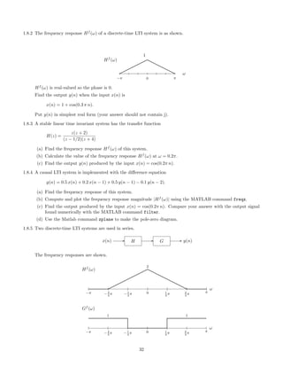
12. >> x = [1 4 2 5]; h = [1 3 -1 2];
>> convmtx(h’,4)*x’
ans =
1
7
13
9
21
-1
10
>> conv(h,x)’
ans =
1
7
13
9
21
-1
10
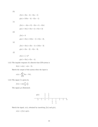
1.3.8 Sketch the convolution of the discrete-time signal x(n)
2
3
2
1
-2 -1 0 1 2 3 4 5 6 n
x(n)
with each of the following signals.
(a) f(n) = 2δ(n) − δ(n − 1)
(b) f(n) = u(n)
(c) f(n) = 0.5
(d) f(n) =
∞
k=−∞
δ(n − 5k)
1.4 Z Transforms
1.4.1 The Z-transform of the discrete-time signal x(n) is
X(z) = −3 z2
+ 2 z−3
Accurately sketch the signal x(n).
1.4.2 Define the discrete-time signal x(n) as
x(n) = −0.3 δ(n + 2) + 2.0 δ(n) + 1.5 δ(n − 3) − δ(n − 5)
12

13. (a) Sketch x(n).
(b) Write the Z-transform X(z).
(c) Define G(z) = z−2
X(z). Sketch g(n).
1.4.3 The signal g(n) is defined by the sketch.
1.4.4 Let x(n) be the length-5 signal
x(n) = {1, 2, 3, 2, 1}
where x(0) is underlined. Sketch the signal corresponding to each of the following Z-transforms.
(a) X(2z)
(b) X(z2
)
(c) X(z) + X(−z)
(d) X(1/z)
1.4.5 Sketch the discrete-time signal x(n) with the Z-transform
X(z) = (1 + 2 z) (1 + 3 z−1
) (1 − z−1
).
1.4.6 Define three discrete-time signals:
a(n) = u(n) − u(n − 4)
b(n) = δ(n) + 2 δ(n − 3)
c(n) = δ(n) − δ(n − 1)
Define three new Z-transforms:
D(z) = A(−z), E(z) = A(1/z), F(z) = A(−1/z)
(a) Sketch a(n), b(n), c(n)
(b) Write the Z-transforms A(z), B(z), C(z)
(c) Write the Z-transforms D(z), E(z), F(z)
(d) Sketch d(n), e(n), f(n)
1.4.7 Find the Z-transform X(z) of the signal
x(n) = 4
1
3
n
u(n) −
2
3
n
u(n).
13

14. 1.4.8 Find the right-sided signal x(n) from the Z-transform
X(z) =
2z + 1
z2 − 5
6 z + 1
6
1.4.9 Consider the LTI system with impulse response
h(n) = 3
2
3
n
u(n)
Find the output y(n) when the input x(n) is
x(n) =
1
2
n
u(n).
1.4.10 A discrete-time LTI system has impulse response
h(n) = −2
1
5
n
u(n)
Find the output signal produced by the system when the input signal is
x(n) = 3
1
2
n
u(n)
1.4.11 The transfer function of a discrete-time LTI system is
H(z) = 2 + 4 z−1
− z−3
.
(a) Sketch the impulse response h(n).
(b) Find the difference equation to describe this system.
(c) Classify the system as BIBO stable/unstable.
1.4.12 Sketch the step response of the system in the previous problem.
(In other words, sketch the output signal when the input signal is the step function u(n).)
What is the steady state value of the step response (as n → ∞)?
1.4.13 Consider the transfer functions of two discrete-time LTI systems,
H1(z) = 1 + 2z−1
+ z−2
,
H2(z) = 1 + z−1
+ z−2
.
(a) If these two systems are cascaded in series, what is the impulse response of the total system?
x(n) - H1(z) - H2(z) - y(n)
(b) If these two systems are combined in parallel, what is the impulse response of the total system?
- H2(z)
- H1(z)
x(n)
?
6
j+ - y(n)
14

15. 1.4.14 Connected systems:
1.4.15 Consider the parallel combination of two LTI systems.
E h2(n)
E h1(n)
x(n)
c
T
l+ E y(n)
You are told that the impulse responses of the two systems are
h1(n) = 3
1
2
n
u(n)
and
h2(n) = 2
1
3
n
u(n)
(a) Find the impulse response h(n) of the total system.
(b) You want to implement the total system as a cascade of two first order systems g1(n) and g2(n). Find
g1(n) and g2(n), each with a single pole, such that when they are connected in cascade, they give the same
system as h1(n) and h2(n) connected in parallel.
x(n) E g1(n) E g2(n) E y(n)
1.4.16 Consider the cascade combination of two LTI systems.
x(n) E SYS 1 E SYS 2 E y(n)
The impulse response of SYS 1 is
h1(n) = δ(n) + 0.5 δ(n − 1) − 0.5 δ(n − 2)
and the transfer function of SYS 2 is
H2(z) = z−1
+ 2 z−2
+ 2 z−3
.
(a) Sketch the impulse response of the total system.
(b) What is the transfer function of the total system?
15

16. 1.5 Inverse Systems
1.5.1 The impulse response of a discrete-time LTI system is
h(n) = −δ(n) + 2
1
2
n
u(n).
(a) Find the impulse response of the stable inverse of this system.
(b) Use MATLAB to numerically verify the correctness of your answer by computing the convolution of h(n)
and the impulse response of the inverse system. You should get δ(n). Include your program and plots with
your solution.
1.5.2 A discrete-time LTI system
x(n) E h(n) E y(n)
has the impulse response
h(n) = δ(n) + 3.5 δ(n − 1) + 1.5 δ(n − 2).
(a) Find the transfer function of the system h(n).
(b) Find the impulse response of the stable inverse of this system.
(c) Use MATLAB to numerically verify the correctness of your answer by computing the convolution of h(n)
and the impulse response of the inverse system. You should get δ(n). Include your program and plots with
your solution.
1.5.3 Consider a discrete-time LTI system with the impulse response
h(n) = δ(n + 1) −
10
3
δ(n) + δ(n − 1).
(a) Find the impulse response g(n) of the stable inverse of this system.
(b) Use MATLAB to numerically verify the correctness of your answer by computing the convolution of h(n)
and the impulse response of the inverse system. You should get δ(n). Include your program and plots with
your solution.
1.5.4 A causal discrete-time LTI system
x(n) E H(z) E y(n)
is described by the difference equation
y(n) −
1
3
y(n − 1) = x(n) − 2 x(n − 1).
What is the impulse response of the stable inverse of this system?
1.6 Difference Equations
1.6.1 A causal discrete-time system is described by the difference equation,
y(n) = x(n) + 3 x(n − 1) + 2 x(n − 4)
(a) What is the transfer function of the system?
16

17. (b) Sketch the impulse response of the system.
1.6.2 Given the impulse response . . .
1.6.3 A causal discrete-time LTI system is implemented using the difference equation
y(n) = x(n) + x(n − 1) + 0.5 y(n − 1)
where x is the input signal, and y the output signal. Find and sketch the impulse response of the system.
1.6.4 Given the impulse response . . .
1.6.5 Given two discrete-time LTI systems described by the difference equations
T1 : y(n) +
1
3
y(n − 1) = x(n) + 2x(n − 1)
T2 : y(n) +
1
3
y(n − 1) = x(n) − 2x(n − 1)
17

18. let T be the cascade of T1 and T2 in series. What is the difference equation describing T? Suppose T1 and T2
are causal systems. Is T causal? Is T stable?
1.6.6 Consider the parallel combination of two causal discrete-time LTI systems.
E SYS 1
E SYS 2
x(n)
c
T
l+ E r(n)
You are told that System 1 is described by the difference equation
y(n) − 0.1 y(n − 1) = x(n) + x(n − 2)
and that System 2 is described by the difference equation
y(n) − 0.1 y(n − 1) = x(n) + x(n − 1).
Find the difference equation of the total system.
1.6.7 Consider a causal discrete-time LTI system described by the difference equation
y(n) −
5
6
y(n − 1) +
1
6
y(n − 2) = 2 x(n) +
2
3
x(n − 1).
(a) Find the transfer function H(z).
(b) Find the impulse response h(n). You may use Matlab to do the partial fraction expansion. See the command
residue. Make a stem plot of h(n) with Matlab.
(c) Plot the magnitude of the frequency response |H(ejω
)| of the system. Use the Matlab command freqz.
1.6.8 A room where echos are present can be modeled as an LTI system that has the following rule:
y(n) =
∞
k=0
2−k
x(n − 10 k)
The output y(n) is made up of delayed versions of the input x(n) of decaying amplitude.
(a) Sketch the impulse response h(n).
(b) What is transfer function H(z)?
(c) Write the corresponding finite-order difference equation.
1.6.9 Echo Canceler. A recorded discrete-time signal r(n) is distorted due to an echo. The echo has a lag of 10
samples and an amplitude of 2/3. That means
r(n) = x(n) +
2
3
x(n − 10)
where x(n) is the original signal. Design an LTI system with impulse response g(n) that removes the echo from
the recorded signal. That means, the system you design should recover the original signal x(n) from the signal
r(n).
(a) Find the impulse response g(n).
(b) Find a difference equation that can be used to implement the system.
18

19. (c) Is the system you designed both causal and stable?
1.6.10 Consider a causal discrete-time LTI system with the impulse response
h(n) =
3
2
3
4
n
u(n) + 2 δ(n − 4)
(a) Make a stem plot of h(n) with Matlab.
(b) Find the transfer function H(z).
(c) Find the difference equation that describes this system.
(d) Plot the magnitude of the frequency response |H(ejω
)| of the system. Use the Matlab command freqz.
1.6.11 Consider a stable discrete-time LTI system described by the difference equation
y(n) = x(n) − x(n − 1) − 2 y(n − 1).
(a) Find the transfer function H(z) and its ROC.
(b) Find the impulse response h(n).
1.6.12 Two LTI systems are connected in series:
E SYS 1 E SYS 2 E
The system SYS 1 is described by the difference equation
y(n) = x(n) + 2 x(n − 1) + x(n − 2)
where x(n) represents the input into SYS 1 and y(n) represents the output of SYS 1.
The system SYS 2 is described by the difference equation
y(n) = x(n) + x(n − 1) + x(n − 2)
where x(n) represents the input into SYS 2 and y(n) represents the output of SYS 2.
(a) What difference equation describes the total system?
(b) Sketch the impulse response of the total system.
1.6.13 Three causal discrete-time LTI systems are used to create the a single LTI system.
x(n) H1
H2
H3
+ y(n)
r(n)
f(n)
g(n)
The difference equations used to implement the systems are:
H1 : r(n) = 2 x(n) −
1
2
r(n − 1)
H2 : f(n) = r(n) −
1
3
f(n − 1)
H3 : g(n) = r(n) −
1
4
r(n − 1)
What is the transfer function Htot(z) for the total system?
19

20. 1.6.14 Given the difference equation...
1.7 Complex Poles
1.7.1 A causal discrete-time LTI system is implemented using the difference equation
y(n) = x(n) − y(n − 2)
where x is the input signal, and y the output signal.
(a) Sketch the pole/zero diagram of the system.
(b) Find and sketch the impulse response of the system.
(c) Classify the system as stable/unstable.
1.7.2 The impulse response of an LTI discrete-time system is
h(n) =
1
2
n
cos
2π
3
n u(n).
Find the difference equation that implements this system.
1.7.3 A causal discrete-time LTI system is implemented using the difference equation
y(n) = x(n) − 4 y(n − 2)
where x is the input signal, and y the output signal.
(a) Sketch the pole/zero diagram of the system.
(b) Find and sketch the impulse response of the system.
(c) Classify the system as stable/unstable.
(d) Find the form of the output signal when the input signal is
x(n) = 2
1
3
n
u(n).
You do not need to compute the constants produced by the partial fraction expansion procedure (PFA)
— you can just leave them as constants: A, B, etc. Be as accurate as you can be in your answer without
actually going through the arithmetic of the PFA.
20

21. 1.7.4 A causal discrete-time LTI system is implemented using the difference equation
y(n) = x(n) −
1
2
x(n − 1) +
1
2
y(n − 1) −
5
8
y(n − 2)
where x is the input signal, and y the output signal.
(a) Sketch the pole/zero diagram of the system.
(b) Find and sketch the impulse response of the system.
(c) Use Matlab to verify your answers to (a) and (b). Use the command residue and zplane. Use the command
filter to compute the impulse response numerically and verify that it is the same as your formula in (b).
1.7.5 A causal discrete-time LTI system is implemented using the difference equation
y(n) = x(n) −
√
2 x(n − 1) + x(n − 2) − 0.5 y(n − 2)
where x is the input signal, and y the output signal.
(a) Find the poles and zeros of the system.
(b) Sketch the pole/zero diagram of the system.
(c) Find the dc gain of the system.
(d) Find the value of the frequency response at ω = π.
(e) Based on parts (a),(b),(c), roughly sketch the frequency response magnitude |Hf
(ω)| of the system.
(f) Suppose the step function u(n) is applied as the input signal to the system. Find the steady state behavior
of the output signal.
(g) Suppose the cosine waveform cos(0.25πn)u(n) is applied as the input signal to the system. Find the steady
state behavior of the output signal.
(h) Find the impulse response of the system. Your answer should not contain j.
1.7.6 A causal discrete-time LTI system is described by the equation
y(n) =
1
4
3
k=0
x(n − k)
where x is the input signal, and y the output signal.
(a) Sketch the impulse response of the system.
(b) How many zeros does the transfer function H(z) have?
(c) What is the dc gain of the system? (Find Hf
(0).)
(d) Find the value of the frequency response at ω = 0.5 π. (Find Hf
(0.5 π).)
(e) Find the value of the frequency response at ω = π. (Find Hf
(π).)
(f) Based on (b), (d) and (e), find the zeros of H(z); and sketch the pole/zero diagram.
(g) Based on the pole/zero diagram, sketch the frequency response magnitude |Hf
(ω)|.
21

22. 1.7.7 The diagrams on the following pages show the impulse responses and pole-zero diagrams of 8 causal discrete-time
LTI systems. But the diagrams are out of order. Match each diagram by filling out the following table.
You should do this problem without using MATLAB or any other computational tools.
In the pole-zero diagrams, the zeros are shown with ‘o’ and the poles are shown by ‘x’.
IMPULSE RESPONSE POLE-ZERO DIAGRAM
1
2
3
4
5
6
7
8
dOrderMatching/Match1
22

23. 0 10 20 30 40
−1
0
1
2
3
IMPULSE RESPONSE 7
0 10 20 30 40
0
0.5
1
1.5
2
IMPULSE RESPONSE 8
0 10 20 30 40
−1
−0.5
0
0.5
1
1.5
IMPULSE RESPONSE 1
0 10 20 30 40
−0.5
0
0.5
1
1.5
IMPULSE RESPONSE 6
0 10 20 30 40
−1
−0.5
0
0.5
1
IMPULSE RESPONSE 5
0 10 20 30 40
0
5
10
15
IMPULSE RESPONSE 2
0 10 20 30 40
0
0.2
0.4
0.6
0.8
1
1.2
IMPULSE RESPONSE 3
0 10 20 30 40
0
0.2
0.4
0.6
0.8
1
1.2
IMPULSE RESPONSE 4
23

24. −1 −0.5 0 0.5 1
−1
−0.5
0
0.5
1
2
ZERO−POLE DIAGRAM 8
−1 −0.5 0 0.5 1
−1
−0.5
0
0.5
1
2
ZERO−POLE DIAGRAM 2
−1 −0.5 0 0.5 1
−1
−0.5
0
0.5
1
2
ZERO−POLE DIAGRAM 5
−1 −0.5 0 0.5 1
−1
−0.5
0
0.5
1
2
ZERO−POLE DIAGRAM 3
−1 −0.5 0 0.5 1
−1
−0.5
0
0.5
1
ZERO−POLE DIAGRAM 4
−1 −0.5 0 0.5 1
−1
−0.5
0
0.5
1
ZERO−POLE DIAGRAM 6
−1 −0.5 0 0.5 1
−1
−0.5
0
0.5
1
ZERO−POLE DIAGRAM 7
−1 −0.5 0 0.5 1
−1
−0.5
0
0.5
1
ZERO−POLE DIAGRAM 1
24

25. 1.7.8 The diagrams on the following pages show the pole-zero diagrams and impulse responses of 8 causal discrete-time
LTI systems. But the diagrams are out of order. Match each diagram by filling out the following table.
You should do this problem without using MATLAB or any other computational tools.
In the pole-zero diagrams, the zeros are shown with ‘o’ and the poles are shown by ‘x’.
POLE-ZERO DIAGRAM IMPULSE RESPONSE
1
2
3
4
5
6
7
8
ero
25

26. −1.5 −1 −0.5 0 0.5 1 1.5
−1
−0.5
0
0.5
1
POLE−ZERO DIAGRAM 2
−1.5 −1 −0.5 0 0.5 1 1.5
−1
−0.5
0
0.5
1
2
POLE−ZERO DIAGRAM 4
−1.5 −1 −0.5 0 0.5 1 1.5
−1
−0.5
0
0.5
1
2
POLE−ZERO DIAGRAM 8
−1.5 −1 −0.5 0 0.5 1 1.5
−1
−0.5
0
0.5
1
2
POLE−ZERO DIAGRAM 6
−1.5 −1 −0.5 0 0.5 1 1.5
−1
−0.5
0
0.5
1
3
POLE−ZERO DIAGRAM 3
−1.5 −1 −0.5 0 0.5 1 1.5
−1
−0.5
0
0.5
1
2
POLE−ZERO DIAGRAM 7
−1.5 −1 −0.5 0 0.5 1 1.5
−1
−0.5
0
0.5
1
2
POLE−ZERO DIAGRAM 5
−1.5 −1 −0.5 0 0.5 1 1.5
−1
−0.5
0
0.5
1
2
POLE−ZERO DIAGRAM 1
26

27. 0 10 20 30 40 50
0
0.2
0.4
0.6
0.8
1
IMPULSE RESPONSE 1
0 10 20 30 40 50
−2
−1
0
1
2
IMPULSE RESPONSE 5
0 10 20 30 40 50
−20
−10
0
10
20
IMPULSE RESPONSE 4
0 10 20 30 40 50
−2
−1
0
1
2
IMPULSE RESPONSE 8
0 10 20 30 40 50
−5
0
5
IMPULSE RESPONSE 7
0 10 20 30 40 50
−1
−0.5
0
0.5
1
IMPULSE RESPONSE 3
0 10 20 30 40 50
−1
−0.5
0
0.5
1
IMPULSE RESPONSE 2
0 10 20 30 40 50
−1
−0.5
0
0.5
1
IMPULSE RESPONSE 6
27

28. 1.7.9 The pole-zero diagrams of eight discrete-time systems are illustrated below. The impulse response h(n) of each
system is also shown, but in a different order. Match each frequency response to its pole-zero diagram by filling
out the table.
POLE-ZERO DIAGRAM IMPULSE RESPONSE
1
2
3
4
5
6
7
8
28

29. −1 −0.5 0 0.5 1
−1
−0.5
0
0.5
1
2
ZERO−POLE DIAGRAM 7
−1 −0.5 0 0.5 1
−1
−0.5
0
0.5
1
2
ZERO−POLE DIAGRAM 8
−1 −0.5 0 0.5 1
−1
−0.5
0
0.5
1
2
ZERO−POLE DIAGRAM 2
−1 −0.5 0 0.5 1
−1
−0.5
0
0.5
1
2
ZERO−POLE DIAGRAM 3
−1 −0.5 0 0.5 1
−1
−0.5
0
0.5
1
ZERO−POLE DIAGRAM 6
−1 −0.5 0 0.5 1
−1
−0.5
0
0.5
1
ZERO−POLE DIAGRAM 4
−1 −0.5 0 0.5 1
−1
−0.5
0
0.5
1
ZERO−POLE DIAGRAM 1
−1 −0.5 0 0.5 1
−1
−0.5
0
0.5
1
ZERO−POLE DIAGRAM 5
29

30. 0 10 20 30 40
−1
−0.5
0
0.5
1
IMPULSE RESPONSE 8
0 10 20 30 40
−6
−4
−2
0
2
4
6
8
IMPULSE RESPONSE 2
0 10 20 30 40
−1
−0.5
0
0.5
1
1.5
IMPULSE RESPONSE 7
0 10 20 30 40
−10
−5
0
5
IMPULSE RESPONSE 4
0 10 20 30 40
0
0.2
0.4
0.6
0.8
1
1.2
IMPULSE RESPONSE 3
0 10 20 30 40
0
5
10
15
20
25
IMPULSE RESPONSE 6
0 10 20 30 40
−1
−0.5
0
0.5
1
IMPULSE RESPONSE 5
0 10 20 30 40
−20
−10
0
10
20
IMPULSE RESPONSE 1
1.7.10 The impulse response of a discrete-time LTI system is given by
h(n) = A (0.7)n
u(n).
Suppose the signal
x(n) = B (0.9)n
u(n)
30

31. is input to the system. A and B are unknown constants. Which of the following could be the output signal y(n)?
Choose all that apply and provide an explanation for your answer.
(a) y(n) = K1 (1.6)n
u(n) + K2 (0.2)n
u(n)
(b) y(n) = K1 (0.7)n
u(−n) + K2 (0.2)n
u(−n)
(c) y(n) = K1 (0.7)n
u(n) + K2 (0.9)n
u(n)
(d) y(n) = K1 (0.7)n
u(n) + K2 (0.2)n
u(−n)
(e) y(n) = K1 (0.7)n
u(n) + K2 (0.2)n
u(n) + K3 (0.9)n
u(n)
(f) y(n) = K1 (0.7)n
u(n) + K2 (0.2)n
u(n) + K3 u(n)
1.7.11 The impulse response of a discrete-time LTI system is given by
h(n) = A (0.7)n
u(n).
Suppose the signal
x(n) = B cos(0.2 π n) u(n)
is input to the system. A and B are unknown constants. Which of the following could be the output signal y(n)?
Choose all that apply and provide an explanation for your answer.
(a) y(n) = K1 (0.7)n
cos(0.2 π n + θ) u(n)
(b) y(n) = K1 (0.14)n
cos(0.5 π n + θ) u(n)
(c) y(n) = K1 (0.14)n
u(n) + K2 cos(0.14 π n + θ) u(n)
(d) y(n) = K1 (0.14)n
u(−n) + K2 cos(0.14 π n + θ) u(n)
(e) y(n) = K1 (0.7)n
u(−n) + K2 cos(0.2 π n + θ) u(n)
(f) y(n) = K1 (0.7)n
u(n) + K2 cos(0.2 π n + θ) u(n)
1.7.12 A causal LTI discrete-time system is implemented using the difference equation
y(n) = b0 x(n) − a1 y(n − 1) − a2 y(n − 2)
where ak, bk are unknown real constants. Which of the following could be the impulse response? Choose all that
apply and provide an explanation for your answer.
(a) h(n) = K1 an
u(n) + K2 bn
u(n)
(b) h(n) = K1 an
u(n) + K2 rn
cos(ω1 n + θ) u(n)
(c) h(n) = K1 rn
cos(ω1 n + θ) u(n)
(d) h(n) = K1 rn
1 cos(ω1 n + θ1) u(n) + K2 rn
2 cos(ω2 n + θ2) u(n) (with ω1 = ω2).
1.8 Frequency Responses
1.8.1 The frequency response Hf
(ω) of a discrete-time LTI system is
Hf
(ω) =
e−jω
−0.4π < ω < 0.4π
0 0.4π < |ω| < π.
Find the output y(n) when the input x(n) is
x(n) = 1.2 cos(0.3 π n) + 1.5 cos(0.5 π n).
Put y(n) in simplest real form (your answer should not contain j).
Hint: Use Euler’s formula and the relation
ejωon
−→ LTI SYSTEM −→ Hf
(ωo) ejωon
31

32. 1.8.2 The frequency response Hf
(ω) of a discrete-time LTI system is as shown.
−π 0
1
π
ω
Hf
(ω)
¨
¨¨¨
¨¨rr
rrr
r
Hf
(ω) is real-valued so the phase is 0.
Find the output y(n) when the input x(n) is
x(n) = 1 + cos(0.3 π n).
Put y(n) in simplest real form (your answer should not contain j).
1.8.3 A stable linear time invariant system has the transfer function
H(z) =
z(z + 2)
(z − 1/2)(z + 4)
(a) Find the frequency response Hf
(ω) of this system.
(b) Calculate the value of the frequency response Hf
(ω) at ω = 0.2π.
(c) Find the output y(n) produced by the input x(n) = cos(0.2π n).
1.8.4 A causal LTI system is implemented with the difference equation
y(n) = 0.5 x(n) + 0.2 x(n − 1) + 0.5 y(n − 1) − 0.1 y(n − 2).
(a) Find the frequency response of this system.
(b) Compute and plot the frequency response magnitude |Hf
(ω)| using the MATLAB command freqz.
(c) Find the output produced by the input x(n) = cos(0.2π n). Compare your answer with the output signal
found numerically with the MATLAB command filter.
(d) Use the Matlab command zplane to make the pole-zero diagram.
1.8.5 Two discrete-time LTI systems are used in series.
x(n) H G y(n)
The frequency responses are shown.
ω
−π −2
3
π −1
3
π 0 1
3
π 2
3
π π
Hf
(ω)
2
ω
−π −2
3
π −1
3
π 0 1
3
π 2
3
π π
Gf
(ω)
1 1
32

33. (a) Accurately sketch the frequency response of the total system.
(b) Find the output signal y(n) produced by the input signal
x(n) = 5 + 3 cos
π
2
n + 2 cos
2π
3
n + 4 (−1)n
.
1.8.6 Three discrete-time LTI systems are combined as illustrated:
x(n) H1
H2
H3
+ y(n)
r(n)
f(n)
g(n)
The frequency responses of the systems are:
ω
−π −2
3
π −1
3
π 0 1
3
π 2
3
π π
Hf
1 (ω)
2
ω
−π −2
3
π −1
3
π 0 1
3
π 2
3
π π
Hf
2 (ω)
1
ω
−π −2
3
π −1
3
π 0 1
3
π 2
3
π π
Hf
3 (ω)
1 1
(a) Accurately sketch the frequency response of the total system.
(b) Find the output signal y(n) produced by the input signal
x(n) = 5 + 3 cos
π
6
n + 2 cos
π
2
n + 4 (−1)n
.
1.8.7 Three discrete-time LTI systems are combined as illustrated:
x(n) H1
H2
H3
+ y(n)
r(n)
f(n)
g(n)
The frequency responses of the systems are:
ω
−π − 2
3 π − 1
3 π 0 1
3 π 2
3 π π
Hf
1 (ω)
1
33

34. ω
−π − 2
3 π − 1
3 π 0 1
3 π 2
3 π π
Hf
2 (ω)
1
ω
−π − 2
3 π − 1
3 π 0 1
3 π 2
3 π π
Hf
3 (ω)
1 1
(a) Accurately sketch the frequency response of the total system.
(b) Find the output signal y(n) produced by the input signal
x(n) = 2 + cos
π
3
n + 3 cos
π
2
n + 0.5 (−1)n
.
1.8.8 The mangitude and phase of the frequency response of a discrete-time LTI system are:
|Hf
(ω)| =
2 for |ω| < 0.5 π
1 for 0.5π < |ω| < π.
∠Hf
(ω) =
0.3 π for − π < ω < 0
−0.3 π for 0 < ω < π.
(a) Sketch the frequency response magnitude |Hf
(ω)| for |ω| ≤ π.
(b) Sketch the frequency response phase ∠Hf
(ω) for |ω| ≤ π.
(c) Find the output signal y(n) produced by the input signal
x(n) = 2 sin(0.2 π n) + 3 cos(0.6 π n + 0.2 π).
1.8.9 The frequency response of a discrete-time LTI system is given by,
Hf
(ω) =



1, |ω| ≤ 0.25 π
0, 0.25 π < |ω| ≤ 0.5π
1, 0.5 π < |ω| ≤ π
(a) Sketch the frequency response.
(b) Find the output signal produced by the input signal
x(n) = 3 + 2 cos(0.3 π n) + 2 cos(0.7 π n) + (−1)n
.
(c) Classify the system as a low-pass filter, high-pass filter, band-pass filter, band-stop filter, or none of these.
1.8.10 The frequency response of a discrete-time LTI system is given by
Hf
(ω) =



−j, 0 < ω ≤ 0.4π
j, −0.4π ≤ ω < 0π
0, 0.4 π < |ω| ≤ π
(a) Sketch the frequency response magnitude |Hf
(ω)| for |ω| ≤ π.
(b) Sketch the frequency response phase ∠Hf
(ω) for |ω| ≤ π.
34

35. (c) Find the output signal y(n) when the input signal is
x(n) = 2 cos(0.3 π n) + 0.7 cos(0.7 π n) + (−1)n
.
Simplify your answer so that it does not contain j.
1.8.11 The frequency response of a real discrete-time LTI system is given by
Hf
(ω) =



0, 0 ≤ |ω| ≤ 0.4π
−j, 0.4π < ω < π
j, −π < ω < −0.4 π
(a) Sketch the frequency response magnitude |Hf
(ω)| for |ω| ≤ π.
(b) Sketch the frequency response phase ∠Hf
(ω) for |ω| ≤ π.
(c) Find the output signal y(n) produced by the input signal
x(n) = 3 + 2 cos(0.3 π n) + 2 cos(0.7 π n).
Simplify your answer so that it does not contain j.
(d) Classify the system as a low-pass filter, high-pass filter, band-pass filter, band-stop filter, or none of these.
1.8.12 The frequency response of a discrete-time LTI system is given by
Hf
(ω) =
2 e−j 1.5 ω
, for |ω| ≤ 0.4π
0, for 0.4 π < |ω| ≤ π
(a) Sketch the frequency response magnitude |Hf
(ω)| for |ω| ≤ π.
(b) Sketch the frequency response phase ∠Hf
(ω) for |ω| ≤ π.
(c) Find the output signal y(n) produced by the input signal
x(n) = 3 + 2 cos(0.3 π n) + 0.7 cos(0.7 π n) + (−1)n
.
Simplify your answer so that it does not contain j.
1.8.13 The frequency response of a discrete-time LTI system is given by
Hf
(ω) =



0, |ω| ≤ 0.25 π
e−j2.5ω
, 0.25 π < |ω| ≤ 0.5π
0, 0.5 π < |ω| ≤ π
(a) Sketch the frequency response magnitude |Hf
(ω)| for |ω| ≤ π.
(b) Sketch the frequency response phase ∠Hf
(ω) for |ω| ≤ π.
(c) Find the output signal produced by the input signal
x(n) = 3 + 2 cos(0.3 π n) + 2 cos(0.7 π n) + (−1)n
.
Simplify your answer so that it does not contain j.
(d) Classify the system as a low-pass filter, high-pass filter, band-pass filter, band-stop filter, or none of these.
1.8.14 The frequency response of a discrete-time LTI system is given by
Hf
(ω) =



2 e−jω
, |ω| ≤ 0.25 π
e−j2ω
, 0.25 π < |ω| ≤ 0.5π
0, 0.5 π < |ω| ≤ π
35

36. (a) Sketch the frequency response magnitude |Hf
(ω)| for |ω| ≤ π.
(b) Sketch the frequency response phase ∠Hf
(ω) for |ω| ≤ π.
(c) Find the output signal produced by the input signal
x(n) = 3 + 2 cos(0.3 π n) + 2 cos(0.7 π n) + (−1)n
.
(d) Is the impulse response of the system real-valued? Explain.
1.8.15 The following figure shows the frequency response magnitudes |Hf
(ω)| of four discrete-time LTI systems (Systems
A, B, C, and D). The signal
x(n) = 2 cos(0.15 π n) u(n − 5) + 2 cos(0.24 π n) u(n − 5)
shown below is applied as the input to each of the four systems. The input signal x(n) and each of the four
output signals are also shown below. But the output signals are out of order. For each of the four systems,
identify which signal is the output signal. Explain your answer.
You should do this problem without using MATLAB or any other computational tools.
System Output signal
A
B
C
D
Output
0 10 20 30 40 50 60 70 80 90 100
−5
0
5
n
INPUTSIGNAL
0 0.25 π 0.5 π 0.75 π π
0
0.2
0.4
0.6
0.8
1
SYSTEMA
ω
0 0.25 π 0.5 π 0.75 π π
0
0.2
0.4
0.6
0.8
1
SYSTEMB
ω
0 0.25 π 0.5 π 0.75 π π
0
0.2
0.4
0.6
0.8
1
1.2
SYSTEMC
ω
0 0.25 π 0.5 π 0.75 π π
0
0.2
0.4
0.6
0.8
1
1.2
SYSTEMD
ω
36

37. 0 10 20 30 40 50 60 70 80 90 100
−5
0
5
n
OUTPUTSIGNAL1
OUTPUT SIGNALS
0 10 20 30 40 50 60 70 80 90 100
−5
0
5
n
OUTPUTSIGNAL2
0 10 20 30 40 50 60 70 80 90 100
−5
0
5
n
OUTPUTSIGNAL3
0 10 20 30 40 50 60 70 80 90 100
−5
0
5
n
OUTPUTSIGNAL4
37

38. 1.8.16 The three discrete-time signals below are each applied to two discrete-time systems to produce a total of six
output signals. The frequency response of each system is shown below. Indicate how each of the six output
signals are produced by completing the table below.
−5 0 5 10 15 20 25
−4
−2
0
2
4
INPUT SIGNAL 1
−5 0 5 10 15 20 25
−4
−2
0
2
4
INPUT SIGNAL 2
−5 0 5 10 15 20 25
−4
−2
0
2
4
INPUT SIGNAL 3
0 0.25 π 0.5 π 0.75 π π
0
1
2
3
4
SYSTEM 1 FREQUENCY RESPONSE
ω
|Hf
1
(ω)|
0 0.25 π 0.5 π 0.75 π π
0
1
2
3
4
SYSTEM 2 FREQUENCY RESPONSE
ω
|Hf
2
(ω)|
Input signal System Output signal
1 1
2 1
3 1
1 2
2 2
3 2
38

39. −5 0 5 10 15 20 25
−4
−2
0
2
4
OUTPUT SIGNAL 2
−5 0 5 10 15 20 25
−4
−2
0
2
4
OUTPUT SIGNAL 4
−5 0 5 10 15 20 25
−4
−2
0
2
4
OUTPUT SIGNAL 3
−5 0 5 10 15 20 25
−4
−2
0
2
4
OUTPUT SIGNAL 6
−5 0 5 10 15 20 25
−4
−2
0
2
4
OUTPUT SIGNAL 5
−5 0 5 10 15 20 25
−4
−2
0
2
4
OUTPUT SIGNAL 1
39

40. 1.8.17 The three discrete-time signals below are each applied to two discrete-time LTI systems to produce a total of
six output signals. The frequency response Hf
(ω) of each system is shown below. Indicate how each of the six
output signals are produced by completing the table below.
Input signal System Output signal
1 1
1 2
2 1
2 2
3 1
3 2
−π −0.5 π 0 0.5 π π
0
0.2
0.4
0.6
0.8
1
SYSTEM 1 FREQUENCY RESPONSE
ω
−π −0.5 π 0 0.5 π π
0
0.2
0.4
0.6
0.8
1
SYSTEM 2 FREQUENCY RESPONSE
ω
40

41. 0 10 20 30 40 50 60 70 80
−1
−0.5
0
0.5
1
INPUT SIGNAL 1
0 10 20 30 40 50 60 70 80
−1
−0.5
0
0.5
1
INPUT SIGNAL 2
0 10 20 30 40 50 60 70 80
−1
−0.5
0
0.5
1
INPUT SIGNAL 3
41

42. 0 10 20 30 40 50 60 70 80
−1
−0.5
0
0.5
1
OUTPUT SIGNAL 1
0 10 20 30 40 50 60 70 80
−1
−0.5
0
0.5
1
OUTPUT SIGNAL 2
0 10 20 30 40 50 60 70 80
−1
−0.5
0
0.5
1
OUTPUT SIGNAL 3
0 10 20 30 40 50 60 70 80
−1
−0.5
0
0.5
1
OUTPUT SIGNAL 4
42

43. 0 10 20 30 40 50 60 70 80
−1
−0.5
0
0.5
1
OUTPUT SIGNAL 5
0 10 20 30 40 50 60 70 80
−1
−0.5
0
0.5
1
OUTPUT SIGNAL 6
1.8.18 Each of the two discrete-time signals below are processed with each of two LTI systems. The frequency response
magnitude |Hf
(ω)| are shown below. Indicate how each of the four output signals are produced by completing
the table below.
Input signal System Output signal
1 1
1 2
2 1
2 2
0 10 20 30 40 50 60
−1
−0.5
0
0.5
1
INPUT SIGNAL 1
0 10 20 30 40 50 60
−1
−0.5
0
0.5
1
INPUT SIGNAL 2
43

44. −π −0.5 π 0 0.5 π π
0
0.2
0.4
0.6
0.8
1
SYSTEM 1 FREQUENCY RESPONSE
ω
−π −0.5 π 0 0.5 π π
0
0.2
0.4
0.6
0.8
1
SYSTEM 2 FREQUENCY RESPONSE
ω
0 10 20 30 40 50 60
−1
−0.5
0
0.5
1
OUTPUT SIGNAL 4
0 10 20 30 40 50 60
−1
−0.5
0
0.5
1
OUTPUT SIGNAL 3
0 10 20 30 40 50 60
−1
−0.5
0
0.5
1
OUTPUT SIGNAL 1
0 10 20 30 40 50 60
−1
−0.5
0
0.5
1
OUTPUT SIGNAL 2
44

45. 1.8.19 Each of the two discrete-time signals below are processed with each of two LTI systems. The frequency response
magnitude |Hf
(ω)| are shown below. Indicate how each of the four output signals are produced by completing
the table below.
Input signal 1 is given by: cos(0.9 π n) u(n − 4)
Input signal 2 is given by: 0.75 cos(0.07 π n) u(n − 4) + 0.25 (−1)n
u(n − 4)
Input signal System Output signal
1 1
1 2
2 1
2 2
0 10 20 30 40 50 60 70 80
−1
0
1
INPUT SIGNAL 1
0 10 20 30 40 50 60 70 80
−1
0
1
INPUT SIGNAL 2
−π −0.5 π 0 0.5 π π
0
0.2
0.4
0.6
0.8
1
SYSTEM 1 FREQUENCY RESPONSE
ω
−π −0.5 π 0 0.5 π π
0
0.2
0.4
0.6
0.8
1
SYSTEM 2 FREQUENCY RESPONSE
ω
45

46. 0 10 20 30 40 50 60 70 80
−1
0
1
OUTPUT SIGNAL 3
0 10 20 30 40 50 60 70 80
−1
0
1
OUTPUT SIGNAL 2
0 10 20 30 40 50 60 70 80
−1
0
1
OUTPUT SIGNAL 4
0 10 20 30 40 50 60 70 80
−1
0
1
OUTPUT SIGNAL 1
1.8.20 Each of the two discrete-time signals below are processed with each of two LTI systems. The frequency response
magnitude |Hf
(ω)| are shown below. Indicate how each of the four output signals are produced by completing
the table below.
Input signal 1 is given by: cos(0.95 π n) u(n − 4)
Input signal 2 is given by: 0.25 cos(0.07 π n) u(n − 4) + 0.75 (−1)n
u(n − 4)
0 10 20 30 40 50 60 70 80
−1
0
1
INPUT SIGNAL 1
0 10 20 30 40 50 60 70 80
−1
0
1
INPUT SIGNAL 2
−π −0.5 π 0 0.5 π π
0
0.2
0.4
0.6
0.8
1
SYSTEM 1 FREQUENCY RESPONSE
ω
−π −0.5 π 0 0.5 π π
0
0.2
0.4
0.6
0.8
1
SYSTEM 2 FREQUENCY RESPONSE
ω
46

47. 0 10 20 30 40 50 60 70 80
−1
0
1
OUTPUT SIGNAL 2
0 10 20 30 40 50 60 70 80
−1
0
1
OUTPUT SIGNAL 4
0 10 20 30 40 50 60 70 80
−1
0
1
OUTPUT SIGNAL 1
0 10 20 30 40 50 60 70 80
−1
0
1
OUTPUT SIGNAL 3
Input signal System Output signal
1 1
1 2
2 1
2 2
1.8.21 Each of the two discrete-time signals below are processed with each of two LTI systems. The frequency response
magnitude |Hf
(ω)| are shown below. Indicate how each of the four output signals are produced by completing
the table below.
Input signal 1: cos(0.15 π n) u(n − 4)
Input signal 2: 0.75 cos(0.1 π n) u(n − 4) + 0.25 cos(0.5 π n) u(n − 4)
Input signal System Output signal
1 1
1 2
2 1
2 2
0 10 20 30 40 50 60 70 80 90
−1
0
1
INPUT SIGNAL 1
0 10 20 30 40 50 60 70 80 90
−1
0
1
INPUT SIGNAL 2
47

48. −π −0.5 π 0 0.5 π π
0
0.2
0.4
0.6
0.8
1
SYSTEM 1 FREQUENCY RESPONSE
ω
−π −0.5 π 0 0.5 π π
0
0.2
0.4
0.6
0.8
1
SYSTEM 2 FREQUENCY RESPONSE
ω
0 10 20 30 40 50 60 70 80 90
−1
0
1
OUTPUT SIGNAL 3
0 10 20 30 40 50 60 70 80 90
−1
0
1
OUTPUT SIGNAL 2
0 10 20 30 40 50 60 70 80 90
−1
0
1
OUTPUT SIGNAL 4
0 10 20 30 40 50 60 70 80 90
−1
0
1
OUTPUT SIGNAL 1
1.8.22 The diagrams on the following pages show the frequency responses magnitudes |Hf
(ω)| and pole-zero diagrams
of 8 causal discrete-time LTI systems. But the diagrams are out of order. Match each diagram by filling out the
following table.
You should do this problem without using MATLAB or any other computational tools.
In the pole-zero diagrams, the zeros are shown with ‘o’ and the poles are shown by ‘x’.
FREQUENCY RESPONSE POLE-ZERO DIAGRAM
1
2
3
4
5
6
7
8
48

49. dOrderMatching/Match2
−1 −0.5 0 0.5 1
0
2
4
6
8
10
12
ω/π
FREQUENCY RESPONSE 4
−1 −0.5 0 0.5 1
0
1
2
3
4
ω/π
FREQUENCY RESPONSE 2
−1 −0.5 0 0.5 1
0
0.5
1
1.5
2
ω/π
FREQUENCY RESPONSE 1
−1 −0.5 0 0.5 1
0
1
2
3
4
ω/π
FREQUENCY RESPONSE 5
−1 −0.5 0 0.5 1
0
1
2
3
4
5
6
7
ω/π
FREQUENCY RESPONSE 8
−1 −0.5 0 0.5 1
0.5
1
1.5
2
2.5
3
ω/π
FREQUENCY RESPONSE 3
−1 −0.5 0 0.5 1
0
1
2
3
4
5
6
ω/π
FREQUENCY RESPONSE 6
−1 −0.5 0 0.5 1
0
0.2
0.4
0.6
0.8
1
1.2
1.4
ω/π
FREQUENCY RESPONSE 7
49

50. −1 −0.5 0 0.5 1
−1
−0.5
0
0.5
1
2
ZERO−POLE DIAGRAM 3
−1 −0.5 0 0.5 1
−1
−0.5
0
0.5
1
ZERO−POLE DIAGRAM 6
−1 −0.5 0 0.5 1
−1
−0.5
0
0.5
1
2
ZERO−POLE DIAGRAM 5
−1 −0.5 0 0.5 1
−1
−0.5
0
0.5
1
2
ZERO−POLE DIAGRAM 2
−1 −0.5 0 0.5 1
−1
−0.5
0
0.5
1
ZERO−POLE DIAGRAM 8
−1 −0.5 0 0.5 1
−1
−0.5
0
0.5
1
ZERO−POLE DIAGRAM 7
−1 −0.5 0 0.5 1
−1
−0.5
0
0.5
1
ZERO−POLE DIAGRAM 4
−1 −0.5 0 0.5 1
−1
−0.5
0
0.5
1
ZERO−POLE DIAGRAM 1
50

51. 1.8.23 The diagrams on the following pages show the frequency responses and pole-zero diagrams of 6 causal discrete-
time LTI systems. But the diagrams are out of order. Match each diagram by filling out the following table.
You should do this problem without using MATLAB or any other computational tools.
In the pole-zero diagrams, the zeros are shown with ‘o’ and the poles are shown by ‘x’.
FREQUENCY RESPONSE POLE-ZERO DIAGRAM
1
2
3
4
5
6
hD
−1 −0.5 0 0.5 1
0
0.2
0.4
0.6
0.8
1
ω/π
FREQUENCY RESPONSE 1
−1 −0.5 0 0.5 1
0
0.2
0.4
0.6
0.8
1
ω/π
FREQUENCY RESPONSE 2
−1 −0.5 0 0.5 1
0
0.2
0.4
0.6
0.8
1
1.2
ω/π
FREQUENCY RESPONSE 3
−1 −0.5 0 0.5 1
0
0.2
0.4
0.6
0.8
1
1.2
ω/π
FREQUENCY RESPONSE 4
−1 −0.5 0 0.5 1
0
0.2
0.4
0.6
0.8
1
1.2
ω/π
FREQUENCY RESPONSE 5
−1 −0.5 0 0.5 1
0
0.2
0.4
0.6
0.8
1
1.2
ω/π
FREQUENCY RESPONSE 6
51

52. −1 −0.5 0 0.5 1
−1
−0.5
0
0.5
1
ZERO−POLE DIAGRAM 5
−1 −0.5 0 0.5 1
−1
−0.5
0
0.5
1
ZERO−POLE DIAGRAM 4
−1 −0.5 0 0.5 1
−1
−0.5
0
0.5
1
ZERO−POLE DIAGRAM 2
−1 −0.5 0 0.5 1
−1
−0.5
0
0.5
1
ZERO−POLE DIAGRAM 1
−1 −0.5 0 0.5 1
−1
−0.5
0
0.5
1
ZERO−POLE DIAGRAM 6
−1 −0.5 0 0.5 1
−1
−0.5
0
0.5
1
ZERO−POLE DIAGRAM 3
1.8.24 The frequency responses and pole-zero diagrams of eight discrete-time LTI systems are illustrated below. But
they are out of order. Match them to each other by filling out the table.
FREQUENCY RESPONSE POLE-ZERO DIAGRAM
1
2
3
4
5
6
7
8
52

53. − π −0.5 π 0 0.5 π π
0
0.5
1
1.5
Frequency Response 8
ω
− π −0.5 π 0 0.5 π π
0
0.5
1
1.5
2
2.5
Frequency Response 2
ω
− π −0.5 π 0 0.5 π π
0
1
2
3
Frequency Response 5
ω
− π −0.5 π 0 0.5 π π
0
1
2
3
Frequency Response 7
ω
− π −0.5 π 0 0.5 π π
0.2
0.4
0.6
0.8
1
1.2
Frequency Response 6
ω
− π −0.5 π 0 0.5 π π
0
1
2
3
4
Frequency Response 1
ω
− π −0.5 π 0 0.5 π π
0
0.5
1
1.5
Frequency Response 3
ω
− π −0.5 π 0 0.5 π π
0
0.5
1
1.5
Frequency Response 4
ω
53

54. −1 0 1
−1
−0.5
0
0.5
1
ZERO−POLE DIAGRAM 7
−1 0 1
−1
−0.5
0
0.5
1
ZERO−POLE DIAGRAM 4
−1 0 1
−1
−0.5
0
0.5
1
ZERO−POLE DIAGRAM 1
−1 0 1
−1
−0.5
0
0.5
1
ZERO−POLE DIAGRAM 6
−1 0 1
−1
−0.5
0
0.5
1
ZERO−POLE DIAGRAM 3
−1 0 1
−1
−0.5
0
0.5
1
ZERO−POLE DIAGRAM 2
−1 0 1
−1
−0.5
0
0.5
1
ZERO−POLE DIAGRAM 8
−1 0 1
−1
−0.5
0
0.5
1
ZERO−POLE DIAGRAM 5
54

55. 1.8.25 The pole-zero diagrams of eight discrete-time systems are illustrated below. The frequency response Hf
(ω) of
each system is also shown, but in a different order. Match each frequency response to its pole-zero diagram by
filling out the table.
−1 −0.5 0 0.5 1
−1
−0.5
0
0.5
1
4
Real Part
ImaginaryPart
POLE−ZERO DIAGRAM 1
−1 −0.5 0 0.5 1
−1
−0.5
0
0.5
1
4
Real Part
ImaginaryPart
POLE−ZERO DIAGRAM 2
−1 −0.5 0 0.5 1
−1
−0.5
0
0.5
1
2
Real Part
ImaginaryPart
POLE−ZERO DIAGRAM 3
−1 −0.5 0 0.5 1
−1
−0.5
0
0.5
1
2
Real Part
ImaginaryPart
POLE−ZERO DIAGRAM 4
−1 −0.5 0 0.5 1
−1
−0.5
0
0.5
1
2
Real Part
ImaginaryPart
POLE−ZERO DIAGRAM 5
−1 −0.5 0 0.5 1
−1
−0.5
0
0.5
1
Real Part
ImaginaryPart POLE−ZERO DIAGRAM 6
−1 −0.5 0 0.5 1
−1
−0.5
0
0.5
1
Real Part
ImaginaryPart
POLE−ZERO DIAGRAM 7
−1 −0.5 0 0.5 1
−1
−0.5
0
0.5
1
Real Part
ImaginaryPart
POLE−ZERO DIAGRAM 8
55

56. −π −0.5 π 0 0.5 π π
0
0.2
0.4
0.6
0.8
1
1.2
FREQUENCY RESPONSE 5
−π −0.5 π 0 0.5 π π
0
0.2
0.4
0.6
0.8
1
FREQUENCY RESPONSE 1
−π −0.5 π 0 0.5 π π
0
0.2
0.4
0.6
0.8
1
1.2
FREQUENCY RESPONSE 4
−π −0.5 π 0 0.5 π π
0
0.2
0.4
0.6
0.8
1
FREQUENCY RESPONSE 3
−π −0.5 π 0 0.5 π π
0
0.2
0.4
0.6
0.8
1
FREQUENCY RESPONSE 7
−π −0.5 π 0 0.5 π π
0
0.2
0.4
0.6
0.8
1
FREQUENCY RESPONSE 2
−π −0.5 π 0 0.5 π π
0
0.2
0.4
0.6
0.8
1
1.2
FREQUENCY RESPONSE 6
−π −0.5 π 0 0.5 π π
0
0.2
0.4
0.6
0.8
1
1.2
FREQUENCY RESPONSE 8
POLE-ZERO DIAGRAM FREQUENCY RESPONSE
1
2
3
4
5
6
7
8
1.9 Summary Problems
1.9.1 The impulse response of an LTI discrete-time system is given by
h(n) = 2 δ(n) + δ(n − 1).
56

57. (a) Find the transfer function of the system.
(b) Find the difference equation with which the system can be implemented.
(c) Sketch the pole/zero diagram of the system.
(d) What is the dc gain of the system? (In other words, what is Hf
(0)?).
(e) Based on the pole/zero diagram sketch the frequency response magnitude |Hf
(ω)|. Mark the value at ω = 0
and ω = π.
(f) Sketch the output of the system when the input x(n) is the constant unity signal, x(n) = 1.
(g) Sketch the output of the system when the input x(n) is the unit step signal, x(n) = u(n).
(h) Find a formula for the output signal when the input signal is
x(n) =
1
2
n
u(n).
1.9.2 A causal LTI system is implemented using the difference equation
y(n) = x(n) +
9
14
y(n − 1) −
1
14
y(n − 2)
(a) What is the transfer function H(z) of this system?
(b) What is the impulse response h(n) of this system?
(c) Use the MATLAB command filter to numerically verify the correctness of your formula for h(n). (Use
this command to numerically compute the first few values of h(n) from the difference equation, and compare
with the formula.)
1.9.3 A causal discrete-time LTI system is implemented using the difference equation
y(n) = x(n) + 0.5 x(n − 1) + 0.2 y(n − 1)
where x is the input signal, and y the output signal.
(a) Sketch the pole/zero diagram of the system.
(b) Find the dc gain of the system.
(c) Find the value of the frequency response at ω = π.
(d) Based on parts (a),(b),(c), roughly sketch the frequency response magnitude of the system.
(e) Find the form of the output signal when the input signal is
x(n) = 2
1
3
n
u(n).
You do not need to compute the constants produced by the partial fraction expansion procedure (PFA) you
can just leave them as constants: A, B, etc. Be as accurate as you can be in your answer without actually
going through the arithmetic of the PFA.
1.9.4 For the causal discrete-time LTI system implemented using the difference equation
y(n) = x(n) + 0.5 x(n − 1) + 0.5 y(n − 1),
(a) Sketch the pole/zero diagram.
(b) Find the dc gain of the system.
(c) Find the output signal produced by the input signal x(n) = 0.5.
(d) Find the value of the frequency response at ω = π.
(e) Find the steady-state output signal produced by the input signal x(n) = 0.6 (−1)n
u(n). (The steady-state
output signal is the output signal after the transients have died out.)
57

58. (f) Validate your answers using Matlab.
1.9.5 A causal discrete-time LTI system is implemented using the difference equation
y(n) = x(n) − x(n − 2) + 0.8 y(n − 1)
where x is the input signal, and y the output signal.
(a) Sketch the pole/zero diagram of the system.
(b) Find the dc gain of the system.
(c) Find the value of the frequency response at ω = π.
(d) Based on parts (a),(b),(c), roughly sketch the frequency response magnitude |Hf
(ω)| of the system.
1.9.6 The impulse response of a discrete-time LTI system is given by
h(n) =
0.25 for 0 ≤ n ≤ 3
0 for other values of n.
Make an accurate sketch of the output of the system when the input signal is
x(n) =
1 for 0 ≤ n ≤ 30
0 for other values of n.
You should do this problem with out using MATLAB, etc.
1.9.7 If a discrete-time LTI system has the transfer function H(z) = 5, then what difference equation implements this
system? Classify this system as memoryless/with memory.
1.9.8 First order difference system: A discrete-time LTI system is implemented using the difference equation
y(n) = 0.5 x(n) − 0.5 x(n − 1).
(a) What is the transfer function H(z) of the system?
(b) What is the impulse response h(n) of the system?
(c) What is the frequency response Hf
(ω) of the system?
(d) Accurately sketch the frequency response magnitude |Hf
(ω)|.
(e) Find the output y(n) when the input signal is the step signal u(n).
(f) Sketch the pole-zero diagram of the system.
(g) Is the system a low-pass filter, high-pass filter, or neither?
1.9.9 A causal discrete-time LTI system is implemented with the difference equation
y(n) = 3 x(n) +
3
2
y(n − 1).
(a) Find the output signal when the input signal is
x(n) = 3 (2)n
u(n).
Show your work.
(b) Is the system stable or unstable?
(c) Sketch the pole-zero diagram of this system.
1.9.10 A causal discrete-time LTI system is described by the equation
y(n) =
1
3
x(n) +
1
3
x(n − 1) +
1
3
x(n − 2)
where x is the input signal, and y the output signal.
58

59. (a) Sketch the impulse response of the system.
(b) What is the dc gain of the system? (Find Hf
(0).)
(c) Sketch the output of the system when the input x(n) is the constant unity signal, x(n) = 1.
(d) Sketch the output of the system when the input x(n) is the unit step signal, x(n) = u(n).
(e) Find the value of the frequency response at ω = π. (Find Hf
(π).)
(f) Find the output of the system produced by the input x(n) = (−1)n
.
(g) How many zeros does the transfer function H(z) have?
(h) Find the value of the frequency response at ω = 2
3 π. (Find Hf
(2 π/3).)
(i) Find the poles and zeros of H(z); and sketch the pole/zero diagram.
(j) Find the output of the system produced by the input x(n) = cos 2
3 πn .
1.9.11 Two-Point Moving Average. A discrete-time LTI system has impulse response
h(n) = 0.5 δ(n) + 0.5 δ(n − 1).
(a) Sketch the impulse response h(n).
(b) What difference equation implements this system?
(c) Sketch the pole-zero diagram of this system.
(d) Find the frequency resposnse Hf
(ω). Find simple expressions for |Hf
(ω)| and ∠Hf
(ω) and sketch them.
(e) Is this a lowpass, highpass, or bandpass filter?
(f) Find the output signal y(n) when the input signal is x(n) = u(n).
Also, x(n) = cos(ωo n) u(n) for what value of ωo?
(g) Find the output signal y(n) when the input signal is x(n) = (−1)n
u(n).
Also, x(n) = cos(ωo n) u(n) for what value of ωo?
1.9.12 Four-Point Moving Average. A discrete-time LTI system has impulse response
h(n) = 0.25 δ(n) + 0.25 δ(n − 1) + 0.25 δ(n − 2) + 0.25 δ(n − 3)
(a) Sketch h(n).
(b) What difference equation implements this system?
(c) Sketch the pole-zero diagram of this system.
(d) Find the frequency resposnse Hf
(ω). Find simple expressions for |Hf
(ω)| and ∠Hf
(ω) and sketch them.
(e) Is this a lowpass, highpass, or bandpass filter?
1.10 Simple System Design
1.10.1 In this problem you are to design a simple causal real discrete-time FIR LTI system with the following properties:
(a) The system should kill the signal cos(0.75 π n)
(b) The system should have unity dc gain. That is, Hf
(0) = 1.
For the system you design:
(a) Find the difference equation to implement the system.
(b) Sketch the impulse response of the system.
(c) Roughly sketch the frequency response magnitude |Hf
(ω)|. Clearly show the nulls of the frequency response.
1.10.2 In this problem you are to design a causal discrete-time LTI system with the following properties:
(a) The transfer function should have two poles. They should be at z = 1/2 and at z = 0.
(b) The system should kill the signal cos(0.75 π n).
59

60. (c) The system should have unity dc gain. That is, Hf
(0) = 1.
For the system you design:
(a) Find the difference equation to implement the system.
(b) Roughly sketch the frequency response magnitude |Hf
(ω)|. What is the value of the frequency response at
ω = π?
(c) Find the output signal produced by the system when the input signal is sin(0.75 π n).
1.10.3 In this problem you are to design a causal discrete-time LTI system with the following properties:
(a) The transfer function should have two poles. They should be at z = j/2 and at z = −j/2.
(b) The system should kill the signal cos(0.5 π n).
(c) The system should have unity dc gain. That is, Hf
(0) = 1.
For the system you design:
(a) Find the difference equation to implement the system.
(b) Roughly sketch the frequency response magnitude |Hf
(ω)|. What is the value of the frequency response at
ω = π?
(c) Find the output signal produced by the system when the input signal is sin(0.5 π n).
1.10.4 In this problem you are to design a simple causal real discrete-time LTI system with the following properties:
(a) The system should kill the signals (−1)n
and cos(0.5 π n)
(b) The system should have unity dc gain. That is, Hf
(0) = 1.
For the system you design:
(a) Find the difference equation to implement the system.
(b) Sketch the impulse response of the system.
(c) Roughly sketch the frequency response magnitude |Hf
(ω)|. Clearly show the nulls of the frequency response.
1.10.5 Design a simple causal real discrete-time LTI system with the properties:
(a) The system should exactly preserve the signal cos(0.5 π n).
(b) The system should annihilate constant signals. That is, the frequency response should have a null at dc.
Hint: It can be done with an impulse response of length 3.
For the system you design:
(a) Find the difference equation to implement the system.
(b) Sketch the impulse response of the system.
(c) Sketch the poles and zeros of the system.
(d) Find and sketch the frequency response magnitude |Hf
(ω)|.
Clearly show the nulls of the frequency response.
60

61. 1.11 Matching
1.11.1 The diagrams on the following pages show the impulse responses, frequency responses, and pole-zero diagrams
of 4 causal discrete-time LTI systems. But the diagrams are out of order. Match each diagram by filling out the
following table.
You should do this problem without using MATLAB or any other computational tools.
In the pole-zero diagrams, the zeros are shown with ‘o’ and the poles are shown by ‘x’.
IMPULSE RESPONSE FREQUENCY RESPONSE POLE-ZERO DIAGRAM
1
2
3
4
hA
0 10 20 30 40
−1
−0.5
0
0.5
1
1.5
2
IMPULSE RESPONSE 1
0 10 20 30 40
−0.5
0
0.5
1
IMPULSE RESPONSE 2
0 10 20 30 40
0
0.2
0.4
0.6
0.8
1
1.2
IMPULSE RESPONSE 3
0 10 20 30 40
−0.5
0
0.5
1
IMPULSE RESPONSE 4
61

62. − π −0.5 π 0 0.5 π π
0
5
10
15
FREQUENCY RESPONSE 2
ω
− π −0.5 π 0 0.5 π π
0
2
4
6
8
FREQUENCY RESPONSE 4
ω
− π −0.5 π 0 0.5 π π
0
2
4
6
8
FREQUENCY RESPONSE 3
ω
− π −0.5 π 0 0.5 π π
0
2
4
6
FREQUENCY RESPONSE 1
ω
−1 −0.5 0 0.5 1
−1
−0.5
0
0.5
1
2
ZERO−POLE DIAGRAM 3
−1 −0.5 0 0.5 1
−1
−0.5
0
0.5
1
2
ZERO−POLE DIAGRAM 1
−1 −0.5 0 0.5 1
−1
−0.5
0
0.5
1
ZERO−POLE DIAGRAM 2
−1 −0.5 0 0.5 1
−1
−0.5
0
0.5
1
ZERO−POLE DIAGRAM 4
62

63. 1.11.2 The diagrams on the following pages show the impulse responses, frequency responses, and pole-zero diagrams
of 4 causal discrete-time LTI systems. But the diagrams are out of order. Match each diagram by filling out the
following table.
You should do this problem without using MATLAB or any other computational tools.
In the pole-zero diagrams, the zeros are shown with ‘o’ and the poles are shown by ‘x’.
IMPULSE RESPONSE FREQUENCY RESPONSE POLE-ZERO DIAGRAM
1
2
3
4
hB
0 10 20 30 40
−1
−0.5
0
0.5
1
1.5
IMPULSE RESPONSE 1
0 10 20 30 40
0
0.5
1
IMPULSE RESPONSE 2
0 10 20 30 40
0
0.2
0.4
0.6
0.8
1
1.2
IMPULSE RESPONSE 3
0 10 20 30 40
0
0.2
0.4
0.6
0.8
1
1.2
IMPULSE RESPONSE 4
63

64. − π −0.5 π 0 0.5 π π
0
5
10
FREQUENCY RESPONSE 4
ω
− π −0.5 π 0 0.5 π π
0
1
2
3
4
FREQUENCY RESPONSE 1
ω
− π −0.5 π 0 0.5 π π
0
5
10
15
FREQUENCY RESPONSE 3
ω
− π −0.5 π 0 0.5 π π
0
1
2
3
4
FREQUENCY RESPONSE 2
ω
−1 −0.5 0 0.5 1
−1
−0.5
0
0.5
1
2
ZERO−POLE DIAGRAM 2
−1 −0.5 0 0.5 1
−1
−0.5
0
0.5
1
2
ZERO−POLE DIAGRAM 1
−1 −0.5 0 0.5 1
−1
−0.5
0
0.5
1
ZERO−POLE DIAGRAM 4
−1 −0.5 0 0.5 1
−1
−0.5
0
0.5
1
ZERO−POLE DIAGRAM 3
64

65. 1.11.3 The diagrams on the following pages show the frequency responses, impulse responses and pole-zero diagrams of
4 causal discrete-time LTI systems. But the diagrams are out of order. Match each diagram by filling out the
following table.
You should do this problem without using MATLAB or any other computational tools.
In the pole-zero diagrams, the zeros are shown with ‘o’ and the poles are shown by ‘x’.
FREQUENCY RESPONSE POLE-ZERO DIAGRAM IMPULSE RESPONSE
1
2
3
4
hC
−1 −0.5 0 0.5 1
0
0.2
0.4
0.6
0.8
1
ω/π
FREQUENCY RESPONSE 1
−1 −0.5 0 0.5 1
0
0.2
0.4
0.6
0.8
1
ω/π
FREQUENCY RESPONSE 2
−1 −0.5 0 0.5 1
0
0.2
0.4
0.6
0.8
1
1.2
ω/π
FREQUENCY RESPONSE 3
−1 −0.5 0 0.5 1
0
0.2
0.4
0.6
0.8
1
1.2
ω/π
FREQUENCY RESPONSE 4
65

66. −1 −0.5 0 0.5 1
−1
−0.5
0
0.5
1
ZERO−POLE DIAGRAM 4
−1 −0.5 0 0.5 1
−1
−0.5
0
0.5
1
ZERO−POLE DIAGRAM 3
−1 −0.5 0 0.5 1
−1
−0.5
0
0.5
1
ZERO−POLE DIAGRAM 2
−1 −0.5 0 0.5 1
−1
−0.5
0
0.5
1
ZERO−POLE DIAGRAM 1
0 10 20 30 40
−0.1
0
0.1
0.2
0.3
IMPULSE RESPONSE 2
0 10 20 30 40
−0.3
−0.2
−0.1
0
0.1
0.2
0.3
IMPULSE RESPONSE 4
0 10 20 30 40
−0.15
−0.1
−0.05
0
0.05
0.1
IMPULSE RESPONSE 1
0 10 20 30 40
−0.2
0
0.2
0.4
0.6
IMPULSE RESPONSE 3
66

67. 1.11.4 The impulse responses, pole-zero diagrams, and frequency responses of eight discrete-time LTI systems are
illustrated below. But they are out of order. Match them to each other by filling out the table.
IMPULSE RESPONSE POLE-ZERO DIAGRAM FREQUENCY RESPONSE
1
2
3
4
5
6
7
8
67

68. 0 10 20 30 40
−1
−0.5
0
0.5
1
IMPULSE RESPONSE 2
0 10 20 30 40
−1
−0.5
0
0.5
1
1.5
IMPULSE RESPONSE 5
0 10 20 30 40
−0.5
0
0.5
1
IMPULSE RESPONSE 1
0 10 20 30 40
0
0.2
0.4
0.6
0.8
1
1.2
IMPULSE RESPONSE 8
0 10 20 30 40
0
0.2
0.4
0.6
0.8
1
1.2
IMPULSE RESPONSE 3
0 10 20 30 40
0
0.2
0.4
0.6
0.8
1
1.2
IMPULSE RESPONSE 4
0 10 20 30 40
−0.5
0
0.5
1
IMPULSE RESPONSE 7
0 10 20 30 40
−1
−0.5
0
0.5
1
IMPULSE RESPONSE 6
68

69. −1 −0.5 0 0.5 1
−1
−0.5
0
0.5
1
2
ZERO−POLE DIAGRAM 6
−1 −0.5 0 0.5 1
−1
−0.5
0
0.5
1
2
ZERO−POLE DIAGRAM 4
−1 −0.5 0 0.5 1
−1
−0.5
0
0.5
1
2
ZERO−POLE DIAGRAM 3
−1 −0.5 0 0.5 1
−1
−0.5
0
0.5
1
2
ZERO−POLE DIAGRAM 2
−1 −0.5 0 0.5 1
−1
−0.5
0
0.5
1
ZERO−POLE DIAGRAM 5
−1 −0.5 0 0.5 1
−1
−0.5
0
0.5
1
ZERO−POLE DIAGRAM 7
−1 −0.5 0 0.5 1
−1
−0.5
0
0.5
1
ZERO−POLE DIAGRAM 1
−1 −0.5 0 0.5 1
−1
−0.5
0
0.5
1
ZERO−POLE DIAGRAM 8
69

70. − π −0.5 π 0 0.5 π π
0
2
4
6
8
10
Frequency Response 8
ω
− π −0.5 π 0 0.5 π π
0
2
4
6
8
10
Frequency Response 6
ω
− π −0.5 π 0 0.5 π π
0
0.5
1
1.5
2
Frequency Response 7
ω
− π −0.5 π 0 0.5 π π
0
2
4
6
8
10
Frequency Response 4
ω
− π −0.5 π 0 0.5 π π
0
5
10
15
20
Frequency Response 2
ω
− π −0.5 π 0 0.5 π π
0
2
4
6
8
10
Frequency Response 1
ω
− π −0.5 π 0 0.5 π π
0
2
4
6
8
10
Frequency Response 5
ω
− π −0.5 π 0 0.5 π π
0
5
10
15
20
Frequency Response 3
ω
1.12 More Problems
1.12.1 The impulse response h(n) of an LTI system is given by
h(n) =
1
2
n
u(n).
70

71. Find and sketch the output y(n) when the input is given by
x(n) = u(n) − u(n − 2).
Simplify your mathematical formula for y(n) as far as you can. Show your work.
1.12.2 The impulse response h(n) of an LTI system is given by
h(n) = δ(n) + δ(n − 2).
Find and sketch the output y(n) when the input is given by
x(n) =
∞
k=−∞
(−1)k
δ(n − 2 k).
Simplify your mathematical formula for y(n) as far as you can. Show your work.
1.12.3 The impulse response h(n) of an LTI system is given by
h(n) = u(n) − u(n − 5).
(a) What is the transfer function H(z) of this system?
(b) What difference equation implements this system?
1.12.4 Feedback Loop Consider the following connection of two discrete-time LTI systems.
E E
h2(n)
E
'
h1(n)
T
+i
You are told that
h1(n) = δ(n) + δ(n − 1), h2(n) =
1
2
δ(n − 1).
(a) Find the impulse response h(n) of the total system.
(b) Sketch h1(n), h2(n), and h(n).
(c) Find the difference equation describing the total system.
1.12.5 Feedback Loop Consider the following interconnection of two causal discrete-time LTI systems
E E
SYS 1
E
'
SYS 2
T
+i
71

72. where SYS 1 is implemented using the difference equation
y(n) = 2 x(n) − 0.5 y(n − 1)
and SYS 2 is implemented using the difference equation
y(n) = 2 x(n) − 0.2 y(n − 1)
Find the impulse response of the total system, htot(n).
Find the difference equation for the total system.
1.12.6 The signal g(n) is given by
g(n) =
1
2
n
u(n − 1)
(a) Sketch g(n).
(b) Find the Z-transform G(z) of the signal g(n) and its region of convergence.
1.12.7 Two discrete-time LTI systems have the following impulse responses
h1(n) =
1
2
n
u(n), h2(n) = −
1
2
n
u(n)
If the two systems are connected in parallel,
- H2(z)
- H1(z)
x(n)
?
6
j+ - y(n)
Find and make an accurate sketch of the impulse response of the total system.
72

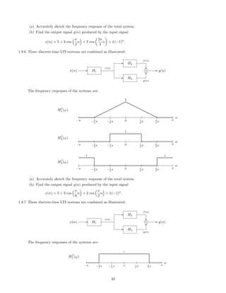
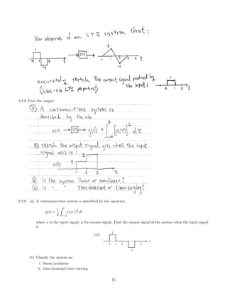
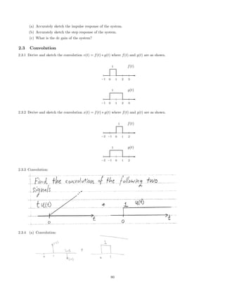
73. 2 Continuous-Time Signals and Systems
2.1 Signals
2.1.1 Make an accurate sketch of each continuous-time signal.
(a)
x(t) = u(t + 1) − u(t),
d
dt
x(t),
t
−∞
x(τ) dτ
(b)
x(t) = e−t
u(t),
d
dt
x(t),
t
−∞
x(τ) dτ
Hint: use the product rule for d
dt (f(t) g(t)).
(c)
x(t) =
1
t
[δ(t − 1) + δ(t + 2)],
t
−∞
x(τ) dτ
(d)
x(t) = r(t) − 2 r(t − 1) + 2 r(t − 3) − r(t − 4)
where r(t) := t u(t) is the ramp function.
(e)
g(t) = x(3 − 2 t), where x(t) is defined as x(t) = 2−t
u(t − 1).
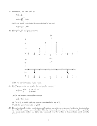
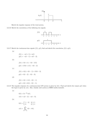
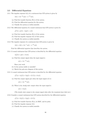
2.1.2 Sketch the continuous-time signals f(t) and g(t) and the product signal f(t) · g(t).
(a)
f(t) = u(t + 4) − u(t − 4), g(t) =
∞
k=−∞
δ(t − 3 k)
(b)
f(t) = cos
π
2
t , g(t) =
∞
k=−∞
δ(t − 2k)
Also write f(t) · g(t) in simple form.
(c)
f(t) = sin
π
2
t , g(t) =
∞
k=−∞
δ(t − 2 k)
(d)
f(t) = sin
π
2
t , g(t) =
∞
k=−∞
δ(t − 2k − 1)
Also write f(t) · g(t) in simple form.
73

74. (e)
f(t) =
1
2
|t|
, g(t) =
∞
k=−∞
δ(t − 2 k).
(f)
f(t) =
∞
k=−∞
(−1)k
δ(t − 0.5 k), g(t) = 2−|t|
2.1.3 Given
f(t) = δ(t) − 2δ(t − 1) + δ(t − 2), g(t) = t u(t)
Define x(t) = f(t) g(t). Accurately sketch x(t).
2.2 System Properties
2.2.1 A continuous-time system is described by the following rule
y(t) = sin(πt) x(t) + cos(πt) x(t − 1)
where x is the input signal, and y is the output signal. Classify the system as:
(a) linear/nonlinear
(b) time-invariant/time-varying
(c) stable/unstable
2.2.2 A continuous-time system is described by the following rule
y(t) =
x(t)
x(t − 1)
.
Classify the system as:
(a) memoryless/with memory
(b) causal/noncausal
(c) linear/nonlinear
(d) time-invariant/time-varying
(e) BIBO stable/unstable
2.2.3 You observe an unknown system and notice that
u(t) − u(t − 1) E S E e−t
u(t)
and that
u(t) − u(t − 2) E S E e−2t
u(t)
Which conclusion can you make?
74

75. (a) The system is LTI.
(b) The system is not LTI.
(c) There is not enough information to decide.
2.2.4 You observe an unknown LTI system and notice that
−1 0 1 2 3 4
1
¡
¡e
e
E h(t) E
−1 0 1 2 3 4
2
¡
¡
¡¡e
e
ee
What is the output of the same LTI system when the input is as shown?
−1 0 1 2 3 4
1
¡
¡e
e¡
¡e
e
E h(t) E
−1 0 1 2 3 4
?
2.2.5 You observe an unknown continuous-time LTI system and notice that
−1 0 1 2 3 4
1
¡
¡e
e
E h(t) E
−1 0 1 2 3 4
2
¡
¡
¡¡e
e
ee
What is the output of the same LTI system when the input is as shown?
−1 0 1 2 3 4
1
¡
¡e
e
e
e¡
¡
E h(t) E
−1 0 1 2 3 4
?
Use the LTI properties and be careful!
2.2.6 You observe an unknown LTI system and notice that
−1 0 1 2 3 4
1
E S E
−1 0 1 2 3 4
1
rr
rr
What is the output of the same LTI system when the input is as shown?
−1 0 1 2 3 4
1
2
1
E S E
−1 0 1 2 3 4
?
2.2.7 Predict the output
75

76. 2.2.8 Find the output.
2.2.9 (a) A continuous-time system is described by the equation,
y(t) =
1
2
t
t−2
(x(τ))2
dτ
where x is the input signal, y the output signal. Find the output signal of the system when the input signal
is
1
-1
0 1 2 5
t
x(t)
(b) Classify the system as:
i. linear/nonlinear
ii. time-invariant/time-varying
76

77. iii. stable/unstable
iv. causa/non-causal
2.2.10 You observe an unknown continuous-time LTI system and notice that
u(t) − u(t − 1) E S E r(t) − 2 r(t − 1) + r(t − 2)
(a) Find and sketch the step response s(t).
(b) Find and sketch the impulse response h(t).
(c) Classify the system as BIBO stable/unstable.
2.2.11 Find the output.
2.2.12 The impulse response h(t) of an LTI system is the triangular pulse shown.
h(t)
-
−1 0 1 2 3
1
d
dd
Suppose the input x(t) is the periodic impulse train
x(t) =
∞
k=−∞
δ(t − k T).
Sketch the output of the system y(t) when
(a) T = 3
(b) T = 2
(c) T = 1.5
2.2.13 Consider an LTI system described by the rule
y(t) = x(t − 5) +
1
2
x(t − 7).
Find and accurately sketch the impulse response h(t) of this system.
77

78. 2.2.14 Consider the LTI system with impulse response
h(t) = t u(t).
(a) Find and sketch the output y(t) when the input x(t) is
x(t) = δ(t) − 2 δ(t − 1) + δ(t − 2).
(b) Classify the system as BIBO stable/unstable.
2.2.15 Consider the LTI system with impulse response
h(t) = δ(t) −
1
4
δ(t − 2).
(a) Find and sketch the output y(t) when the input x(t) is
x(t) = 2−t
u(t).
(b) Classify the system as BIBO stable/unstable.
2.2.16 Consider the continuous-time LTI system with impulse response
h(t) = δ(t − 1).
(a) Find and sketch the output y(t) when the input x(t) is the impulse train with period 2,
x(t) =
∞
k=−∞
δ(t − 2k).
(b) Classify the system as BIBO stable/unstable.
2.2.17 (a) The integrator:
(b) Same (a), but system is defined as
y(t) =
t
t−1
x(τ) dτ
2.2.18 A continuous-time LTI system is described by the equation,
y(t) =
1
2
t
t−2
x(τ) dτ
where x is the input signal, y the output signal.
(a) Write in words what this system does to the input signal.
(b) Accurately sketch the impulse response of the system.
(c) What is the dc gain of the system?
78

79. 2.2.19 A continuous-time LTI system is described by the equation,
y(t) =
t
t−1
x(τ) dτ +
1
2
t−1
t−3
x(τ) dτ
where x is the input signal, y the output signal.
(a) Accurately sketch the impulse response of the system.
(b) Accurately sketch the step response of the system.
(c) What is the dc gain of the system?
2.2.20 You observe a continuous-time LTI system and notice that
1
0 1 2 3
t
H
1
0 1 2 3
t
(a) Accurately sketch the output produced by the following input signal.
1
0 1 2 3
t
H ?
(b) Accurately sketch the step response of the system.
(c) Accurately sketch the impulse response of the system.
2.2.21 Differentiator.
2.2.22 A left-sided signal.
2.2.23 A continuous-time LTI system is described by the equation,
y(t) =
1
5
t−2
t−4
x(τ) dτ
where x is the input signal, y the output signal.
79

80. (a) Accurately sketch the impulse response of the system.
(b) Accurately sketch the step response of the system.
(c) What is the dc gain of the system?
2.3 Convolution
2.3.1 Derive and sketch the convolution v(t) = f(t) ∗ g(t) where f(t) and g(t) are as shown.
f(t)
-
−1 0 1 2 3
1
g(t)
-
−1 0 1 2 3
1
2.3.2 Derive and sketch the convolution x(t) = f(t) ∗ g(t) where f(t) and g(t) are as shown.
f(t)
-
−2 −1 0 1 2
1
g(t)
-
−2 −1 0 1 2
1
2.3.3 Convolution:
2.3.4 (a) Convolution:
80

81. (b) Convolution:
2.3.5 Find and sketch the convolution x(t) = f(t) ∗ g(t) where
f(t) = u(t), g(t) = 3 e−2t
u(t)
2.3.6 Find and sketch the convolution x(t) = f(t) ∗ g(t) where
f(t) = et
u(−t), g(t) = e−t
u(t)
2.3.7 Sketch the continuous-time signals f(t), g(t).
Find and sketch the convolution y(t) = f(t) ∗ g(t).
f(t) = e−t
u(t),
g(t) = e−t
u(t)
2.3.8 Using the convolution integral, find the convolution of the signal f(t) = e−2t
u(t) with itself.
e−2t
u(t) ∗ e−2t
u(t) = ?
2.3.9 Find and sketch the convolution of
g(t) = e−2t
u(t)
and
1
0 1 2 3 4 5
t
f(t)
2.3.10 Sketch the continuous-time signals f(t), g(t).
Find and sketch the convolution y(t) = f(t) ∗ g(t).
f(t) = u(t + 2) − u(t − 2)
g(t) =
∞
k=−∞
δ(t − 3 k)
2.3.11 Sketch the convolution of the following two signals.
1
0 1 2 3 4 5
t
f(t)
1
0 1 2 3 4 5
t
g(t)
81

82. 2.3.12 Consider the cascade connection of two continuous-time LTI systems
x(t) E SYS 1 E SYS 2 E y(t)
with the following impulse responses,
h1(t)
-
−1 0 1 2 3
1
h2(t)
-
−1 0 3
1
−1
Accurately sketch the impulse response of the total system.
82

83. 2.3.13 Two continuous-time LTI systems are connected in cascade.
x(t) h1(t) h2(t) y(t)
The impulse responses of the two systems are:
1
-1
0 3 4 5
t
h1(t)
1
-1
0 1 3 5
t
h2(t)
Sketch the impulse response of the total system.
2.3.14 Two continuous-time LTI systems are connected in cascade.
x(t) h1(t) h2(t) y(t)
The impulse responses of the two systems are:
0 t
1
2
h1(t)
0 t3
(1)1
−1
2
h2(t)
Sketch the impulse response of the total system. (The convolution of h1(t) and h2(t).)
2.3.15 Two continuous-time LTI systems are connected in cascade.
x(t) h1(t) h2(t) y(t)
The impulse responses of the two systems are:
0 t
1
2
h1(t)
83

84. 0 t
(2)
1
1
2
h2(t)
Sketch the impulse response of the total system.
2.3.16 Sketch the convolution of the following two signals.
1
0 1 2 3 4 5
t
f(t)
1
0 1 2 3 4 5
t
g(t)
2.3.17 Sketch the continuous-time signals f(t), g(t); find and sketch the convolution f(t) ∗ g(t).
(a)
f(t) = −u(t + 1) + u(t)
g(t) = −u(t − 1) + u(t − 2).
(b)
f(t) = δ(t + 1) − δ(t − 2.5)
g(t) = 2 δ(t + 1.5) − δ(t − 2)
(c)
f(t) = δ(t) + δ(t − 1) + 2 δ(t − 2)
g(t) = δ(t − 2) − δ(t − 3).
(d)
f(t) = δ(t + 1.2) − δ(t − 1)
g(t) = δ(t + 0.3) − δ(t − 1).
2.3.18 The impulse response of a continuous-time LTI system is given by h(t). Find and sketch the output y(t) when
the input is given by x(t). Also, classify each system as BIBO stable/unstable.
(a)
h(t) = 2 e−3t
u(t).
x(t) = u(t − 2) − u(t − 3).
(b)
h(t) =
1 − |t| |t| ≤ 1
0 |t| ≥ 1
x(t) =
∞
k=−∞
δ(t − 4 k).
84

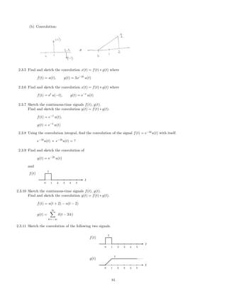
85. (c)
h(t) = e−t
u(t)
x(t) = u(t) − u(t − 2),
(d)
h(t) = cos (πt) u(t).
x(t) = u(t) − u(t − 3).
2.4 Laplace Transform
You may use MATLAB. The residue and roots commands should be useful for some of the following problems.
2.4.1 Given h(t), find H(s) and its region of convergence (ROC).
h(t) = 5e−4t
u(t) + 2e−3t
u(t)
2.4.2 Given H(s), use partial fraction expansion to expand it (by hand). You may use the Matlab command residue
to verify your result. Find the causal impulse response corresponding to H(s).
(a)
H(s) =
s + 4
s2 + 5s + 6
(b)
H(s) =
s − 1
2s2 + 3s + 1
2.4.3 Let
f(t) = e−t
u(t), g(t) = e−2t
u(t)
Use the Laplace transform to find the convolution of these two signals, y(t) = f(t) ∗ g(t).
2.4.4 Let
f(t) = e−t
u(t), g(t) = e−t
u(t)
Use the Laplace transform to find and sketch the convolution of these two signals, y(t) = f(t) ∗ g(t). [Yes, f(t)
and g(t) are the same here.]
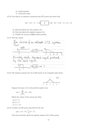
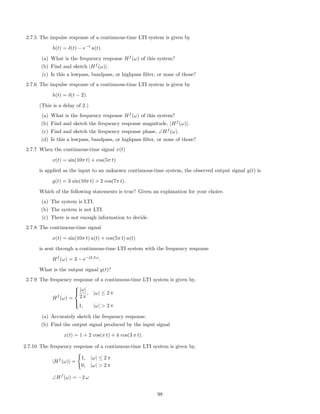
2.4.5 The impulse response of a continuous-time LTI system is given by
h(t) =
1
2
t
u(t).
Sketch h(t) and find the transfer function H(s) of the system.
2.4.6 Let r(t) denote the ramp function, r(t) = t u(t). If the signal g(t) is defined as g(t) = r(t − 2), then what is the
Laplace transform of g(t)?
85

86. 2.5 Differential Equations
2.5.1 The impulse response h(t) of a continuous-time LTI system is given by
h(t) = 3 e−2t
u(t) − e−3t
u(t).
(a) Find the transfer function H(s) of the system.
(b) Find the differential equation for this system.
(c) Classify the system as stable/unstable.
2.5.2 The differential equation of a causal continuous-time LTI system is given by
y (t) + y (t) − 2 y(t) = x(t)
(a) Find the transfer function H(s) of the system.
(b) Find the impulse response h(t) of this system.
(c) Classify the system as stable/unstable.
2.5.3 The impulse response of a continuous-time LTI system is given by
h(t) = δ(t) + 2 e−t
u(t) − e−2t
u(t)
Find the differential equation that describes the system.
2.5.4 A causal continuous-time LTI system is described by the differential equation
2 y (t) + y(t) = 3 x(t).
(a) Find the output signal when the input signal is
x(t) = 5 e−3 t
u(t).
Show your work.
(b) Is the system stable or unstable?
(c) Sketch the pole-zero diagram of this system.
2.5.5 A causal continuous-time LTI system is described by the differential equation
y (t) + 4 y (t) + 3 y(t) = 2 x (t) + 3 x(t)
(a) Find the output signal y(t) when the input signal x(t) is
x(t) = 3 e−2t
u(t).
(b) What is the steady state output when the input signal is
x(t) = 3 u(t).
(The steady state output is the output signal value after the transients have died out.)
2.5.6 Consider a causal continuous-time LTI system described by the differential equation
y (t) + 3 y (t) + 2 y(t) = 2 x (t)
(a) Find the transfer function H(s), its ROC, and its poles.
(b) Find the impulse response h(t).
(c) Classify the system as stable/unstable.
86

87. (d) Find the output of the system when the input signal is
x(t) = 2 u(t).
2.5.7 A causal continuous-time LTI system is described by the differential equation
y (t) + 5 y (t) + 4 y(t) = 3 x (t) + 6 x(t)
(a) Find the impulse response h(t).
(b) Find the output signal y(t) when the input signal x(t) is as shown:
x(t)
-
−1 0 1 2 3
1
2.5.8 Differential equation:
2.5.9 Impulse response:
2.5.10 Consider a continuous-time LTI system with the impulse response
h(t) = e−3t
u(t) + 2 e−t
u(t)
(a) Find the differential equation that describes the system.
(b) Sketch the pole-zero diagram.
(c) Find the output signal y(t) produced by the input signal
x(t) = e−2t
u(t).
You may leave the residues as unspecified constants.
87

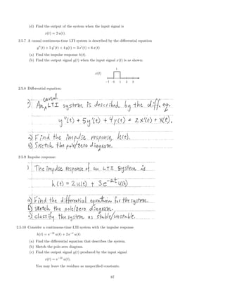
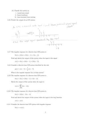
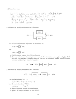
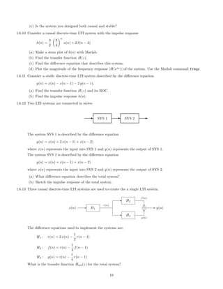
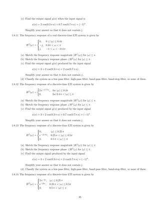
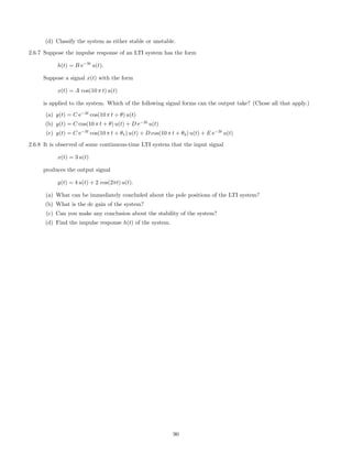
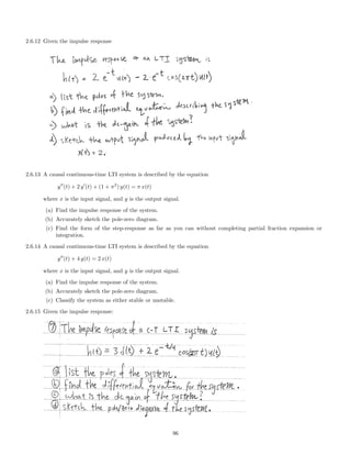
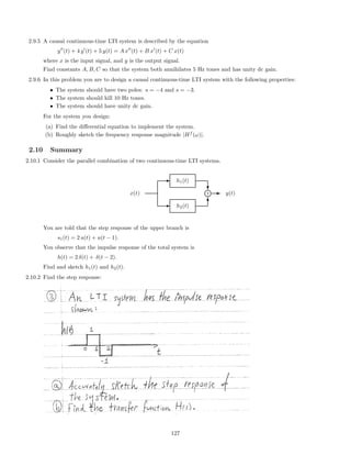
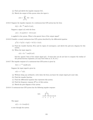
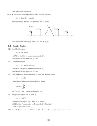
88. 2.5.11 A causal LTI system is described by the differential equation
y (t) + 7 y (t) + 12 y(t) = 3 x (t) + 2 x(t).
(a) Find the transfer function H(s) and the ROC of H(s).
(b) List the poles of H(s).
(c) Find the impulse response h(t).
(d) Classify the system as stable/unstable.
(e) Fnd the output y(t) when the input is
x(t) = e−t
u(t) + e−2t
u(t).
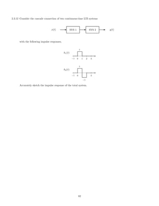
2.5.12 Given the two LTI systems described the the differential equations:
T1 : y (t) + 3 y (t) + 7 y(t) = 2 x (t) + x(t)
T2 : y (t) + y (t) + 4 y(t) = x (t) − 3 x(t)
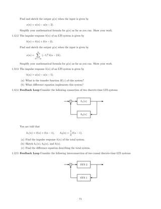
(a) Let T be the cascade of T1 and T2, T[x(t)] = T2[T1[x(t)]], as shown in the diagram.
x(t) E SYS 1 E SYS 2 E y(t)
What are H1(s), H2(s), Htot(s), the transfer functions of T1, T2 and T? What is the differential equation
describing the total system T?
(b) Let T be the sum of T1 and T2, T[x(t)] = T2[x(t)] + T1[x(t)], as shown in the diagram.
E SYS 2
E SYS 1
x(t)
c
T
l+ E y(t)
What is Htot(s), the transfer function of the total system T? What is the differential equation describing
the total system T?
2.5.13 Given a causal LTI system described by
y (t) +
1
3
y(t) = 2 x(t)
find H(s). Given the input x(t) = e−2t
u(t), find the output y(t) without explicitly finding h(t). (Use Y (s) =
H(s)X(s), and find y(t) from Y (s).)
2.5.14 The impulse response of an LTI continuous-time system is given by
h(t) = 3 e−t
u(t) + 2 e−2 t
u(t) + e−t
u(t)
(a) Find the transfer function of the system.
(b) Find the differential equation with which the system can be implemented.
(c) List the poles of the system.
(d) What is the dc gain of the system?
(e) Sketch the output signal produced by input signal, x(t) = 1.
(f) Find the steady-state output produced by input signal, x(t) = u(t).
88

89. 2.6 Complex Poles
2.6.1 Consider a causal continuous-time LTI system described by the differential equation
y (t) + y(t) = x(t).
(a) Find the transfer function H(s), its ROC, and its poles.
(b) Find the impulse response h(t).
(c) Classify the system as stable/unstable.
(d) Find the step response of the system.
2.6.2 Given the impulse response of a continuous-time LTI system, find the transfer function H(s), the ROC of H(s),
and the poles of the system. Use Euler’s formula! Also find the differential equation describing each system.
(a) h(t) = sin(3 t) u(t)
(b) h(t) = e−t/2
sin(3 t) u(t)
(c) h(t) = e−t
u(t) + e−t/2
cos(3 t) u(t)
2.6.3 A causal continuous-time LTI system is described by the equation
y (t) + 2 y (t) + 5 y(t) = x(t)
where x is the input signal, and y is the output signal.
(a) Find the impulse response of the system.
(b) Accurately sketch the pole-zero diagram.
(c) What is the dc gain of the system?
(d) Classify the system as either stable or unstable.
(e) Write down the form of the step response of the system, as far as it can be determined without actually
calculating the resides. (You do not need to complete the partial fraction expansion).
2.6.4 Given a causal LTI system described by the differential equation find H(s), the ROC of H(s), and the impulse
response h(t) of the system. Classify the system as stable/unstable. List the poles of H(s). You should the
Matlab residue command for this problem.
(a) y + 3 y + 2 y = x + 6 x + 6 x
(b) y + 8 y + 46 y + 68y = 10 x + 53 x + 144 x
2.6.5 It is observed of some continuous-time LTI system that the input signal
x(t) = e−2 t
u(t)
produces the output signal
y(t) = 0.5 e−2 t
u(t) + 2 e−3t
cos(2πt) u(t).
What can be concluded about the pole positions of the LTI system?
2.6.6 A causal continuous-time LTI system is described by the equation
y (t) + 4 y (t) + 5 y(t) = x (t) + 2x(t)
where x is the input signal, and y is the output signal.
(a) Find the impulse response of the system.
(b) Accurately sketch the pole-zero diagram.
(c) What is the dc gain of the system?
89

90. (d) Classify the system as either stable or unstable.
2.6.7 Suppose the impulse response of an LTI system has the form
h(t) = B e−3t
u(t).
Suppose a signal x(t) with the form
x(t) = A cos(10 π t) u(t)
is applied to the system. Which of the following signal forms can the output take? (Chose all that apply.)
(a) y(t) = C e−3t
cos(10 π t + θ) u(t)
(b) y(t) = C cos(10 π t + θ) u(t) + D e−3t
u(t)
(c) y(t) = C e−3t
cos(10 π t + θ1) u(t) + D cos(10 π t + θ2) u(t) + E e−3t
u(t)
2.6.8 It is observed of some continuous-time LTI system that the input signal
x(t) = 3 u(t)
produces the output signal
y(t) = 4 u(t) + 2 cos(2πt) u(t).
(a) What can be immediately concluded about the pole positions of the LTI system?
(b) What is the dc gain of the system?
(c) Can you make any conclusion about the stability of the system?
(d) Find the impulse response h(t) of the system.
90

91. 2.6.9 The following diagrams indicate the pole locations of six continuous-time LTI systems. Match each with the
corresponding impulse response with out actually computing the Laplace transform.
POLE-ZERO DIAGRAM IMPULSE RESPONSE
1
2
3
4
5
6
−1 0 1
−5
0
5 #1
−1 0 1
−5
0
5 #2
−1 0 1
−5
0
5 #3
−1 0 1
−5
0
5 #4
−1 0 1
−5
0
5 #5
−1 0 1
−5
0
5 #6
0 2 4
−1
0
1
2
A
0 2 4
−1
0
1
2
B
0 2 4
−1
0
1
2
C
0 2 4
−1
0
1
2
D
0 2 4
−1
0
1
2
E
0 2 4
−1
0
1
2
F
91

92. 2.6.10 The impulse responses of eight causal continuous-time systems are illustrated below, along with the pole/zero
diagram of each system. But they are out of order. Match the figures with each other by completing the table.
IMPULSE RESPONSE POLE-ZERO DIAGRAM
1
2
...
8
−1 0 1 2 3 4 5 6
0
0.2
0.4
0.6
0.8
1
IMPULSE RESPONSE 1
−1 0 1 2 3 4 5 6
0
0.2
0.4
0.6
0.8
1
IMPULSE RESPONSE 2
−1 0 1 2 3 4 5 6
0
5
10
15
20
IMPULSE RESPONSE 3
−1 0 1 2 3 4 5 6
−0.5
0
0.5
1
IMPULSE RESPONSE 4
−1 0 1 2 3 4 5 6
−0.5
0
0.5
1
IMPULSE RESPONSE 5
−1 0 1 2 3 4 5 6
−0.5
0
0.5
1
IMPULSE RESPONSE 6
−1 0 1 2 3 4 5 6
−15
−10
−5
0
5
10
15
IMPULSE RESPONSE 7
TIME (SEC)
−1 0 1 2 3 4 5 6
−10
0
10
20
IMPULSE RESPONSE 8
TIME (SEC)
92

93. −3 −2 −1 0 1 2 3
−20
−10
0
10
20
REAL
IMAG
POLE/ZERO DIAGRAM 6
−3 −2 −1 0 1 2 3
−20
−10
0
10
20
REAL
IMAG
POLE/ZERO DIAGRAM 1
−3 −2 −1 0 1 2 3
−20
−10
0
10
20
REAL
IMAG
POLE/ZERO DIAGRAM 8
−3 −2 −1 0 1 2 3
−20
−10
0
10
20
REAL
IMAG
POLE/ZERO DIAGRAM 3
−3 −2 −1 0 1 2 3
−20
−10
0
10
20
REAL
IMAG
POLE/ZERO DIAGRAM 2
−3 −2 −1 0 1 2 3
−20
−10
0
10
20
REAL
IMAG
POLE/ZERO DIAGRAM 7
−3 −2 −1 0 1 2 3
−20
−10
0
10
20
REAL
IMAG
POLE/ZERO DIAGRAM 4
−3 −2 −1 0 1 2 3
−20
−10
0
10
20
REAL
IMAG
POLE/ZERO DIAGRAM 5
93

94. 2.6.11 The first six seconds of the impulse responses of eight causal continuous-time systems are illustrated below, along
with the pole/zero diagram of each system. But they are out of order. Match the figures with each other by
completing the table.
IMPULSE RESPONSE POLE-ZERO DIAGRAM
1
2
...
8
−1 0 1 2 3 4 5 6
0
0.5
1
1.5
2
IMPULSE RESPONSE 1
−1 0 1 2 3 4 5 6
0
0.2
0.4
0.6
0.8
1
IMPULSE RESPONSE 2
−1 0 1 2 3 4 5 6
0
0.2
0.4
0.6
0.8
1
IMPULSE RESPONSE 3
−1 0 1 2 3 4 5 6
−0.5
0
0.5
1
IMPULSE RESPONSE 4
−1 0 1 2 3 4 5 6
−0.5
0
0.5
1
IMPULSE RESPONSE 5
−1 0 1 2 3 4 5 6
−1
−0.5
0
0.5
1
IMPULSE RESPONSE 6
−1 0 1 2 3 4 5 6
−1
−0.5
0
0.5
1
IMPULSE RESPONSE 7
TIME (SEC)
−1 0 1 2 3 4 5 6
−10
0
10
20
IMPULSE RESPONSE 8
TIME (SEC)
94

95. −3 −2 −1 0 1 2 3
−20
−10
0
10
20
REAL
IMAG
POLE/ZERO DIAGRAM 5
−3 −2 −1 0 1 2 3
−20
−10
0
10
20
REAL
IMAG
POLE/ZERO DIAGRAM 4
−3 −2 −1 0 1 2 3
−20
−10
0
10
20
REAL
IMAG
POLE/ZERO DIAGRAM 7
−3 −2 −1 0 1 2 3
−20
−10
0
10
20
REAL
IMAG
POLE/ZERO DIAGRAM 2
−3 −2 −1 0 1 2 3
−20
−10
0
10
20
REAL
IMAG
POLE/ZERO DIAGRAM 3
−3 −2 −1 0 1 2 3
−20
−10
0
10
20
REAL
IMAG
POLE/ZERO DIAGRAM 8
−3 −2 −1 0 1 2 3
−20
−10
0
10
20
REAL
IMAG
POLE/ZERO DIAGRAM 1
−3 −2 −1 0 1 2 3
−20
−10
0
10
20
REAL
IMAG
POLE/ZERO DIAGRAM 6
95

96. 2.6.12 Given the impulse response
2.6.13 A causal continuous-time LTI system is described by the equation
y (t) + 2 y (t) + (1 + π2
) y(t) = π x(t)
where x is the input signal, and y is the output signal.
(a) Find the impulse response of the system.
(b) Accurately sketch the pole-zero diagram.
(c) Find the form of the step-response as far as you can without completing partial fraction expansion or
integration.
2.6.14 A causal continuous-time LTI system is described by the equation
y (t) + 4 y(t) = 2 x(t)
where x is the input signal, and y is the output signal.
(a) Find the impulse response of the system.
(b) Accurately sketch the pole-zero diagram.
(c) Classify the system as either stable or unstable.
2.6.15 Given the impulse response:
96

97. 2.7 Frequency Response
2.7.1 The frequency response of a continuous-time LTI system is given by
Hf
(ω) =
1 for |ω| < 4 π
0 for |ω| ≥ 4 π.
(a) Sketch the frequency response.
(b) Find the output y(t) of the system when the input is
x(t) = 3 cos(2 π t) + 6 sin(5 π t).
2.7.2 The signal x(t) in the previous problem is filtered with a continuous-time LTI system having the following
frequency response. Find the output y(t).
−4π 0
6
4π
ω
Hf
(ω)
t
t
t
tt
2.7.3 Consider the cascade combination of two continuous-time LTI systems.
x(t) E SYS 1 E SYS 2 E y(t)
The frequency response of SYS 1 is
Hf
1 (ω) =
1 for |ω| 6 π
0 for |ω| ≥ 6 π.
The frequency response of SYS 2 is
Hf
2 (ω) =
0 for |ω| 4 π
1 for |ω| ≥ 4 π.
(a) Sketch the frequency responses of each of the two systems.
(b) If the input signal is
x(t) = 2 cos(3π t) − 3 sin(5π t) + 4 cos(7π t)
what is the output signal y(t)?
(c) What is the frequency response of the total system?
2.7.4 The frequency response Hf
(ω) of a continuous-time LTI system is given by
Hf
(ω) =
1
j ω
.
(a) Find the output y(t) when the input is given by
x(t) = cos(2 t) + sin(4 t).
(b) Sketch the magnitude of the frequency response, |Hf
(ω)|, and the phase of the frequency response, ∠Hf
(ω).
(c) Classify the system as stable/unstable and give a brief explanation for your answer.
97

98. 2.7.5 The impulse response of a continuous-time LTI system is given by
h(t) = δ(t) − e−t
u(t).
(a) What is the frequency response Hf
(ω) of this system?
(b) Find and sketch |Hf
(ω)|.
(c) Is this a lowpass, bandpass, or highpass filter, or none of those?
2.7.6 The impulse response of a continuous-time LTI system is given by
h(t) = δ(t − 2).
(This is a delay of 2.)
(a) What is the frequency response Hf
(ω) of this system?
(b) Find and sketch the frequency response magnitude, |Hf
(ω)|.
(c) Find and sketch the frequency response phase, ∠Hf
(ω).
(d) Is this a lowpass, bandpass, or highpass filter, or none of those?
2.7.7 When the continuous-time signal x(t)
x(t) = sin(10π t) + cos(5π t)
is applied as the input to an unknown continuous-time system, the observed output signal y(t) is
y(t) = 3 sin(10π t) + 2 cos(7π t).
Which of the following statements is true? Given an explanation for your choice.
(a) The system is LTI.
(b) The system is not LTI.
(c) There is not enough information to decide.
2.7.8 The continuous-time signal
x(t) = sin(10π t) u(t) + cos(5π t) u(t)
is sent through a continuous-time LTI system with the frequency response
Hf
(ω) = 3 − e−j2.3 ω
.
What is the output signal y(t)?
2.7.9 The frequency response of a continuous-time LTI system is given by,
Hf
(ω) =



|ω|
2 π
, |ω| ≤ 2 π
1, |ω| 2 π
(a) Accurately sketch the frequency response.
(b) Find the output signal produced by the input signal
x(t) = 1 + 2 cos(π t) + 4 cos(3 π t).
2.7.10 The frequency response of a continuous-time LTI system is given by,
|Hf
(ω)| =
1, |ω| ≤ 2 π
0, |ω| 2 π
∠Hf
(ω) = −2 ω
98

99. (a) Accurately sketch the frequency response magnitude |Hf
(ω)| and phase ∠Hf
(ω).
(b) Find the output signal produced by the input signal
x(t) = 1 + 2 cos(π t) + 4 cos(3 π t).
2.7.11 Consider the cascade connection of two copies of the same continuous-time LTI system:
x(t) E h1(t) E h1(t) E y(t)
where h1(t) is as shown:
h1(t)
-
−1 0 1 2 3
1
(a) Find the frequency response Hf
1 (ω).
(b) Find the frequency response of the total system Hf
tot(ω).
2.7.12 Suppose H is an ideal lowpass filter with cut-off frequency ωo. Suppose H is connected in series with another
copy of itself,
x(t) −→ H −→ H −→ y(t)
Find and sketch the frequency response of the total system.
2.7.13 Two continuous-time LTI systems are connected in cascade.
x(t) h1(t) h2(t) y(t)
The impulse responses of the two systems are:
h1(t) = 10 sinc (10 t)
h2(t) = δ(t) − 5 sinc (5 t)
(a) Accurately sketch the frequency response of the total system.
(b) Find the impulse response h(t) of the total system.
2.7.14 Consider the continuous-time LTI system that delays its input by 2.5 seconds,
y(t) = x(t − 2.5).
(a) Accurately sketch the impulse response h(t).
(b) Find the frequency response Hf
(ω).
(c) Accurately sketch the frequency response magnitude |Hf
(ω)|.
(d) Accurately sketch the frequency response phase ∠Hf
(ω).
(e) Find the output signal produced by the input signal
x(t) = 1 + 2 cos(π t) + 4 cos(3 π t).
99

100. 2.7.15 An echo can be modeled with a causal LTI system described by the equation
y(t) = x(t) −
1
2
x(t − 10).
(a) Find the impulse response h(t).
(b) Classify the system as stable/unstable.
(c) Find the frequency response Hf
(ω) and sketch |Hf
(ω)|2
.
2.7.16 Two continuous-time LTI systems are connected in cascade.
x(t) E h1(t) E h2(t) E y(t)
The impulse responses are given by
h1(t) = δ(t − 0.5)
h2(t) = e−2t
u(t)
(a) Find the impulse response h(t) of the total system.
(b) Find the frequency response Hf
(ω) of the total system.
(c) Find the steady-state output signal y(t) when the input is
x(t) = cos(2 π t) u(t).
2.7.17 Consider a continuous-time LTI system with the frequency response:
Hf
(ω) =
j ω, |ω| ≤ 4π
0, |ω| 4π
(a) Sketch the frequency response magnitude |Hf
(ω)|.
(b) Sketch the frequency response phase ∠Hf
(ω).
(c) Find the output signal produced by the input signal
x(t) = 2 + cos(πt) + 0.5 sin(2πt) + 3 cos(6πt).
Simplify your answer so that it does not contain j. Show your work.
(d) Based on (c) explain why this system may be called a low-pass differentiator.
2.7.18 Find the output:
100

101. 2.7.19 Sketch the frequency response:
2.7.20 Given the frequency response
101

102. 102

103. 2.7.21 Match the impulse response h(t) of a continuous-time LTI system with the correct plot of its frequency response
|Hf
(ω)|. Explain how you obtain your answer.
−0.5 0 0.5 1 1.5 2 2.5 3 3.5 4 4.5 5
−1
−0.5
0
0.5
1
t
IMPULSE RESPONSE
−8 −6 −4 −2 0 2 4 6 8
0
0.2
0.4
0.6
0.8
1
ω
FREQUENCYRESPONSEA
−8 −6 −4 −2 0 2 4 6 8
0
0.2
0.4
0.6
0.8
1
ω
FREQUENCYRESPONSEB
−8 −6 −4 −2 0 2 4 6 8
0
0.2
0.4
0.6
0.8
1
ω
FREQUENCYRESPONSEC
−8 −6 −4 −2 0 2 4 6 8
0
0.2
0.4
0.6
0.8
1
ω
FREQUENCYRESPONSED
103

104. 2.7.22 For the impulse response h(t) illustrated in the previous problem, identify the correct diagram of the poles of
H(s). Explain how you obtain your answer.
−2 0 2
−10
−5
0
5
10
#1
Real part
Imagpart
−2 0 2
−10
−5
0
5
10
#2
Real part
Imagpart
−2 0 2
−10
−5
0
5
10
#3
Real part
Imagpart
−2 0 2
−10
−5
0
5
10
#4
Real partImagpart
104

105. 2.7.23 The figure shows the pole diagrams and frequency responses of four continuous-time LTI systems. But they are
out of order. Match each pole diagram with its frequency response.
POLE-ZERO DIAGRAM FREQUENCY RESPONSE
1
2
3
4
−3 −2.5 −2 −1.5 −1 −0.5 0 0.5
−20
−10
0
10
20
POLE−ZERO DIAGRAM 1
−6 −4 −2 0 2 4 6
0.2
0.4
0.6
0.8
1
1.2
FREQUENCY RESPONSE 3
−3 −2.5 −2 −1.5 −1 −0.5 0 0.5
−20
−10
0
10
20
POLE−ZERO DIAGRAM 2
−6 −4 −2 0 2 4 6
0.05
0.1
0.15
0.2
0.25
0.3
0.35
0.4
FREQUENCY RESPONSE 1
−3 −2.5 −2 −1.5 −1 −0.5 0 0.5
−20
−10
0
10
20
POLE−ZERO DIAGRAM 3
−6 −4 −2 0 2 4 6
0.1
0.2
0.3
0.4
0.5
0.6
FREQUENCY RESPONSE 2
−3 −2.5 −2 −1.5 −1 −0.5 0 0.5
−20
−10
0
10
20
POLE−ZERO DIAGRAM 4
−6 −4 −2 0 2 4 6
0.1
0.2
0.3
0.4
0.5
0.6
FREQUENCY RESPONSE 4
FREQUENCY (Hz)
105

106. 2.7.24 The diagrams on the following pages show the pole-zero diagrams and frequency responses of 8 causal continuous-
time LTI systems. But the diagrams are out of order. Match each diagram by filling out the following table.
In the pole-zero diagrams, the zeros are shown with ‘o’ and the poles are shown by ×.
POLE-ZERO DIAGRAM FREQUENCY RESPONSE
1
2
3
4
5
6
7
8
−6 −4 −2 0 2 4 6
−10
−5
0
5
10
POLE−ZERO DIAGRAM 2
−6 −4 −2 0 2 4 6
−10
−5
0
5
10
POLE−ZERO DIAGRAM 5
−6 −4 −2 0 2 4 6
−10
−5
0
5
10
POLE−ZERO DIAGRAM 8
−6 −4 −2 0 2 4 6
−10
−5
0
5
10
POLE−ZERO DIAGRAM 7
−6 −4 −2 0 2 4 6
−10
−5
0
5
10
POLE−ZERO DIAGRAM 3
−6 −4 −2 0 2 4 6
−10
−5
0
5
10
POLE−ZERO DIAGRAM 4
−6 −4 −2 0 2 4 6
−10
−5
0
5
10
POLE−ZERO DIAGRAM 6
−6 −4 −2 0 2 4 6
−10
−5
0
5
10
POLE−ZERO DIAGRAM 1
106

107. −20 −10 0 10 20
0
0.2
0.4
0.6
0.8
1
FREQUENCY RESPONSE 4
−20 −10 0 10 20
0
0.2
0.4
0.6
0.8
1
FREQUENCY RESPONSE 8
−20 −10 0 10 20
0
0.2
0.4
0.6
0.8
1
FREQUENCY RESPONSE 6
−20 −10 0 10 20
0
0.2
0.4
0.6
0.8
1
FREQUENCY RESPONSE 5
−20 −10 0 10 20
0
0.2
0.4
0.6
0.8
1
FREQUENCY RESPONSE 2
−20 −10 0 10 20
0
0.2
0.4
0.6
0.8
1
FREQUENCY RESPONSE 7
−20 −10 0 10 20
0
0.2
0.4
0.6
0.8
1
FREQUENCY RESPONSE 1
−20 −10 0 10 20
0
0.2
0.4
0.6
0.8
1
FREQUENCY RESPONSE 3
107

108. 2.7.25 The frequency responses of eight causal continuous-time systems are illustrated below, along with the pole/zero
diagram of each system. But they are out of order. Match the figures with each other by completing a table.
FREQUENCY RESPONSE POLE-ZERO DIAGRAM
1
2
3
4
5
6
7
8
−20 −10 0 10 20
0
0.2
0.4
0.6
0.8
1
FREQUENCY RESPONSE 3
−20 −10 0 10 20
0
0.2
0.4
0.6
0.8
1
FREQUENCY RESPONSE 1
−20 −10 0 10 20
0
0.2
0.4
0.6
0.8
1
FREQUENCY RESPONSE 7
−20 −10 0 10 20
0
0.2
0.4
0.6
0.8
1
FREQUENCY RESPONSE 2
−20 −10 0 10 20
0
0.2
0.4
0.6
0.8
1
FREQUENCY RESPONSE 5
−20 −10 0 10 20
0
0.2
0.4
0.6
0.8
1
FREQUENCY RESPONSE 6
−20 −10 0 10 20
0
0.2
0.4
0.6
0.8
1
FREQUENCY RESPONSE 8
−20 −10 0 10 20
0
0.2
0.4
0.6
0.8
1
FREQUENCY RESPONSE 4
108

109. −6 −4 −2 0 2 4 6
−10
−5
0
5
10
POLE−ZERO DIAGRAM 2
−6 −4 −2 0 2 4 6
−10
−5
0
5
10
POLE−ZERO DIAGRAM 5
−6 −4 −2 0 2 4 6
−10
−5
0
5
10
POLE−ZERO DIAGRAM 8
−6 −4 −2 0 2 4 6
−10
−5
0
5
10
POLE−ZERO DIAGRAM 7
−6 −4 −2 0 2 4 6
−10
−5
0
5
10
POLE−ZERO DIAGRAM 3
−6 −4 −2 0 2 4 6
−10
−5
0
5
10
POLE−ZERO DIAGRAM 4
−6 −4 −2 0 2 4 6
−10
−5
0
5
10
POLE−ZERO DIAGRAM 6
−6 −4 −2 0 2 4 6
−10
−5
0
5
10
POLE−ZERO DIAGRAM 1
109

110. 2.7.26 The frequency responses of eight causal continuous-time systems are illustrated below, along with the pole/zero
diagram of each system. But they are out of order. Match the figures with each other by completing the table
(copy the table into your answer book).
FREQUENCY RESPONSE POLE-ZERO DIAGRAM
1
2
3
4
5
6
7
8
−20 −10 0 10 20
0
0.2
0.4
0.6
0.8
1
FREQUENCY RESPONSE 4
−20 −10 0 10 20
0
0.2
0.4
0.6
0.8
1
FREQUENCY RESPONSE 8
−20 −10 0 10 20
0
0.2
0.4
0.6
0.8
1
FREQUENCY RESPONSE 6
−20 −10 0 10 20
0
0.2
0.4
0.6
0.8
1
FREQUENCY RESPONSE 5
−20 −10 0 10 20
0
0.2
0.4
0.6
0.8
1
FREQUENCY RESPONSE 2
−20 −10 0 10 20
0
0.2
0.4
0.6
0.8
1
FREQUENCY RESPONSE 7
−20 −10 0 10 20
0
0.2
0.4
0.6
0.8
1
FREQUENCY RESPONSE 1
−20 −10 0 10 20
0
0.2
0.4
0.6
0.8
1
FREQUENCY RESPONSE 3
110

111. −6 −4 −2 0 2 4 6
−10
−5
0
5
10
POLE−ZERO DIAGRAM 2
−6 −4 −2 0 2 4 6
−10
−5
0
5
10
POLE−ZERO DIAGRAM 5
−6 −4 −2 0 2 4 6
−10
−5
0
5
10
POLE−ZERO DIAGRAM 8
−6 −4 −2 0 2 4 6
−10
−5
0
5
10
POLE−ZERO DIAGRAM 7
−6 −4 −2 0 2 4 6
−10
−5
0
5
10
POLE−ZERO DIAGRAM 3
−6 −4 −2 0 2 4 6
−10
−5
0
5
10
POLE−ZERO DIAGRAM 4
−6 −4 −2 0 2 4 6
−10
−5
0
5
10
POLE−ZERO DIAGRAM 6
−6 −4 −2 0 2 4 6
−10
−5
0
5
10
POLE−ZERO DIAGRAM 1
111

112. 2.7.27 The figure shows the impulse responses and frequency responses of four continuous-time LTI systems. But they
are out of order. Match the impulse response to its frequency response magnitude, and explain your answer.
IMPULSE RESPONSE FREQUENCY RESPONSE
1
2
3
4
−1 0 1 2 3 4 5 6
−1
−0.5
0
0.5
1
IMPULSE RESPONSE 1
−10 −5 0 5 10
0
0.2
0.4
0.6
FREQUENCY RESPONSE 1
−1 0 1 2 3 4 5 6
−1
−0.5
0
0.5
1
IMPULSE RESPONSE 2
−10 −5 0 5 10
0
0.2
0.4
0.6
FREQUENCY RESPONSE 3
−1 0 1 2 3 4 5 6
−1
−0.5
0
0.5
1
IMPULSE RESPONSE 3
−10 −5 0 5 10
0
0.2
0.4
0.6
FREQUENCY RESPONSE 2
−1 0 1 2 3 4 5 6
−1
−0.5
0
0.5
1
IMPULSE RESPONSE 4
TIME (SEC)
−10 −5 0 5 10
0
0.2
0.4
0.6
FREQUENCY RESPONSE 4
FREQUENCY (Hz)
112

113. 2.7.28 The figure shows the impulse responses and frequency responses of four continuous-time LTI systems. But they
are out of order. Match each impulse response with its frequency response.
IMPULSE RESPONSE FREQUENCY RESPONSE
1
2
3
4
−1 0 1 2 3 4 5 6
−1
−0.5
0
0.5
1
IMPULSE RESPONSE 1
−10 −5 0 5 10
0.2
0.4
0.6
0.8
1
1.2
FREQUENCY RESPONSE 3
−1 0 1 2 3 4 5 6
−1
−0.5
0
0.5
1
IMPULSE RESPONSE 2
−10 −5 0 5 10
0.05
0.1
0.15
0.2
0.25
0.3
0.35
0.4
FREQUENCY RESPONSE 4
FREQUENCY (Hz)
−1 0 1 2 3 4 5 6
−1
−0.5
0
0.5
1
IMPULSE RESPONSE 3
−10 −5 0 5 10
0.1
0.2
0.3
0.4
0.5
0.6
FREQUENCY RESPONSE 1
−1 0 1 2 3 4 5 6
−1
−0.5
0
0.5
1
IMPULSE RESPONSE 4
TIME (SEC)
−10 −5 0 5 10
0.1
0.2
0.3
0.4
0.5
0.6
FREQUENCY RESPONSE 2
113

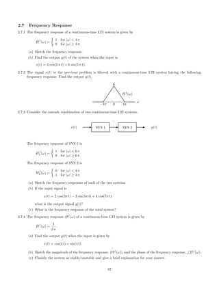
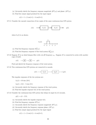
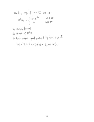
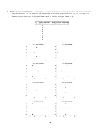
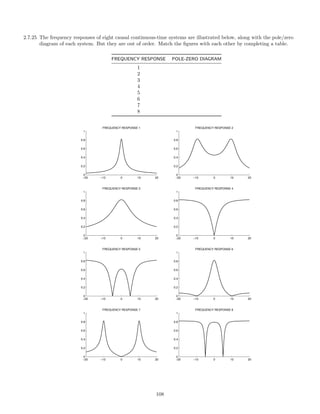
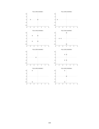
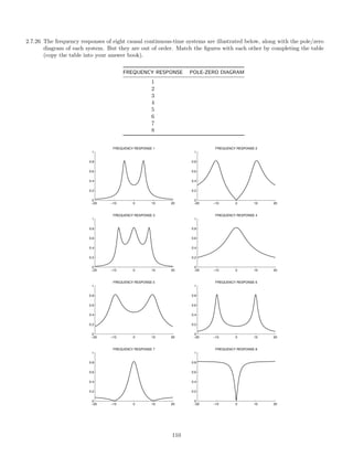
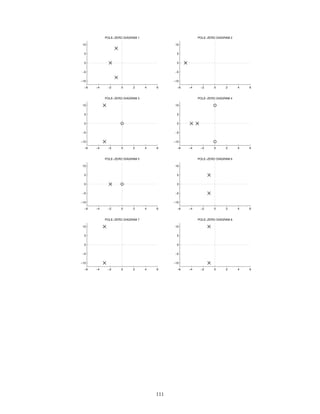
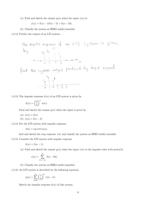
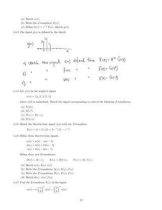
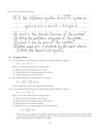
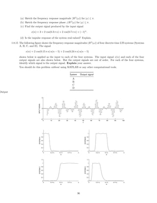
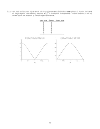
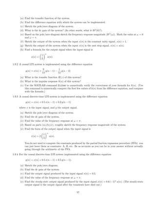
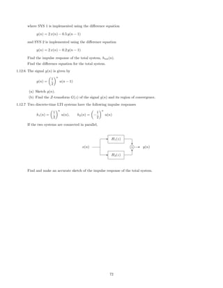
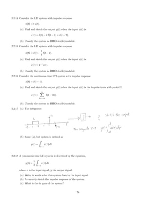
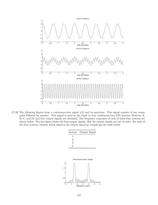
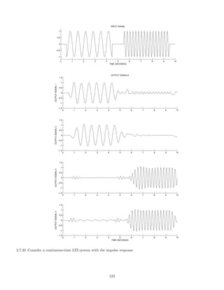
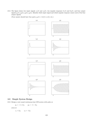
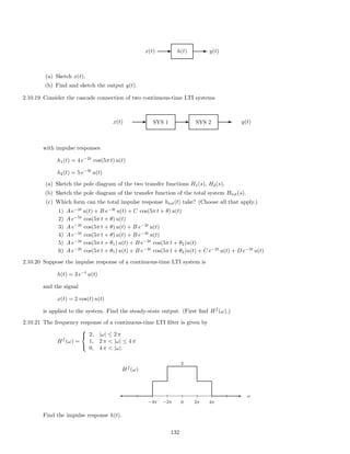
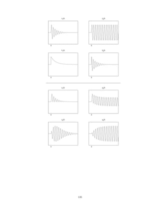
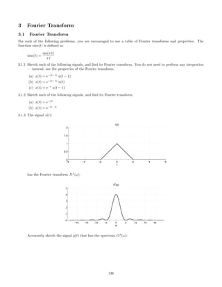
114. 2.7.29 A signal x(t), comprised of three components,
x(t) = 1 + 2 cos(πt) + 0.5 cos(10πt)
is illustrated here:
0 2 4 6 8 10
−4
−2
0
2
4
x(t) [INPUT SIGNAL]
t [SEC.]
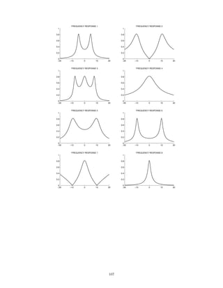
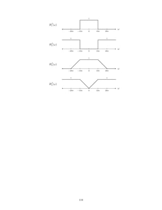
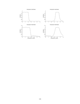
This signal, x(t), is filtered with each of six different continuous-time LTI filters. The frequency response of each
of the six systems are shown below. (For |ω| 3π, each frequency response has the value it has at |ω| = 3π.)
−3π −2π −π 0 π 2π 3π
0
0.5
1
FREQUENCY RESPONSE 1
ω
−3π −2π −π 0 π 2π 3π
0
0.5
1
FREQUENCY RESPONSE 2
ω
−3π −2π −π 0 π 2π 3π
0
0.5
1
FREQUENCY RESPONSE 3
ω
−3π −2π −π 0 π 2π 3π
0
0.5
1
FREQUENCY RESPONSE 4
ω
−3π −2π −π 0 π 2π 3π
0
0.5
1
FREQUENCY RESPONSE 5
ω
−3π −2π −π 0 π 2π 3π
0
0.5
1
FREQUENCY RESPONSE 6
ω
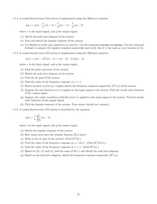
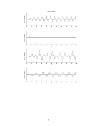
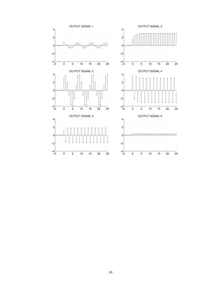
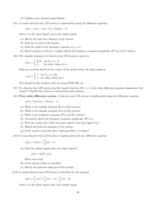
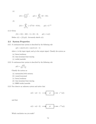
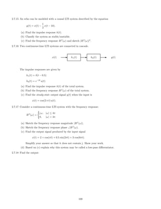
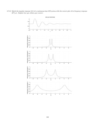
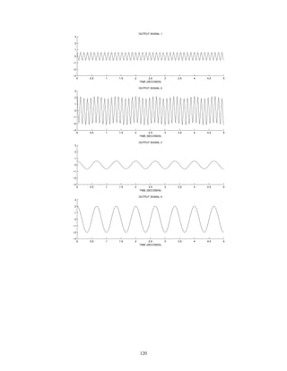
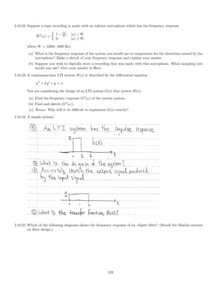
The six output signals are shown below, but they are not numbered in the same order.
114

115. 0 2 4 6 8 10
−4
−2
0
2
4
OUTPUT SIGNAL 1
t [SEC.]
0 2 4 6 8 10
−4
−2
0
2
4
OUTPUT SIGNAL 2
t [SEC.]
0 2 4 6 8 10
−4
−2
0
2
4
OUTPUT SIGNAL 3
t [SEC.]
0 2 4 6 8 10
−4
−2
0
2
4
OUTPUT SIGNAL 4
t [SEC.]
0 2 4 6 8 10
−4
−2
0
2
4
OUTPUT SIGNAL 5
t [SEC.]
0 2 4 6 8 10
−4
−2
0
2
4
OUTPUT SIGNAL 6
t [SEC.]
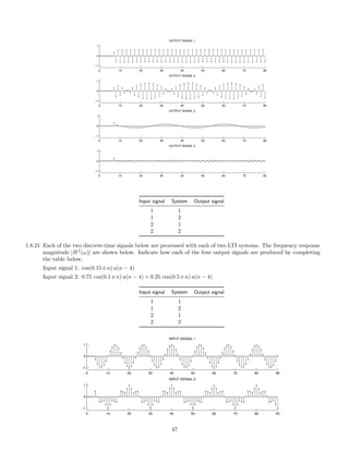
Match each output signal to the system that was used to produce it by completing the table.
System Output signal
1
2
3
4
5
6
115

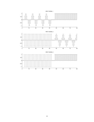
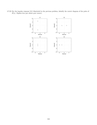
116. 2.7.30 A signal x(t), comprised of three components,
x(t) = 1 + 0.5 cos(πt) + 2 cos(6πt)
is illustrated here:
0 2 4 6 8 10
−4
−2
0
2
4
x(t) [INPUT SIGNAL]
t [SEC.]
This signal, x(t), is filtered with each of six different continuous-time LTI filters. The frequency response of each
of the six systems are shown below. (For |ω| 3π, each frequency response has the value it has at |ω| = 3π.)
−3π −2π −π 0 π 2π 3π
0
0.5
1
FREQUENCY RESPONSE 1
ω
−3π −2π −π 0 π 2π 3π
0
0.5
1
FREQUENCY RESPONSE 2
ω
−3π −2π −π 0 π 2π 3π
0
0.5
1
FREQUENCY RESPONSE 3
ω
−3π −2π −π 0 π 2π 3π
0
0.5
1
FREQUENCY RESPONSE 4
ω
−3π −2π −π 0 π 2π 3π
0
0.5
1
FREQUENCY RESPONSE 5
ω
−3π −2π −π 0 π 2π 3π
0
0.5
1
FREQUENCY RESPONSE 6
ω
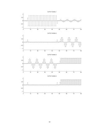
The six output signals are shown below, but they are not numbered in the same order.
116

117. 0 2 4 6 8 10
−4
−2
0
2
4
OUTPUT SIGNAL 1
t [SEC.]
0 2 4 6 8 10
−4
−2
0
2
4
OUTPUT SIGNAL 2
t [SEC.]
0 2 4 6 8 10
−4
−2
0
2
4
OUTPUT SIGNAL 3
t [SEC.]
0 2 4 6 8 10
−4
−2
0
2
4
OUTPUT SIGNAL 4
t [SEC.]
0 2 4 6 8 10
−4
−2
0
2
4
OUTPUT SIGNAL 5
t [SEC.]
0 2 4 6 8 10
−4
−2
0
2
4
OUTPUT SIGNAL 6
t [SEC.]
Match each output signal to the system that was used to produce it by completing the table.
System Output signal
1
2
3
4
5
6
117

118. 2.7.31 Each of the two continuous-time signals below are processed with each of four LTI systems. The two input
signals, illustrated below, are given by:
Input signal 1: 0.6 cos(3πt) + 2 cos(17πt)
Input signal 2: 2 cos(3πt) + 0.6 cos(17πt)
The frequency responses Hf
(ω) are shown below. Indicate how each of the output signals are produced by
completing the table below (copy the table onto your answer sheet). Note: one of the output signals illustrated
below will appear twice in the table (there are seven distinct output signals).
Input signal System Output signal
1 1
1 2
1 3
1 4
2 1
2 2
2 3
2 4
0 0.5 1 1.5 2 2.5 3 3.5 4 4.5 5
−3
−2
−1
0
1
2
3
INPUT SIGNAL 1
TIME (SECONDS)
0 0.5 1 1.5 2 2.5 3 3.5 4 4.5 5
−3
−2
−1
0
1
2
3
INPUT SIGNAL 2
TIME (SECONDS)
118

119. ω
−20π −10π 0 10π 20π
Hf
1 (ω)
1
ω
−20π −10π 0 10π 20π
Hf
2 (ω)
1 1
ω
−20π −10π 0 10π 20π
Hf
3 (ω)
1
ω
−20π −10π 0 10π 20π
Hf
4 (ω)
1 1
119

120. 0 0.5 1 1.5 2 2.5 3 3.5 4 4.5 5
−3
−2
−1
0
1
2
3
OUTPUT SIGNAL 1
TIME (SECONDS)
0 0.5 1 1.5 2 2.5 3 3.5 4 4.5 5
−3
−2
−1
0
1
2
3
OUTPUT SIGNAL 2
TIME (SECONDS)
0 0.5 1 1.5 2 2.5 3 3.5 4 4.5 5
−3
−2
−1
0
1
2
3
OUTPUT SIGNAL 3
TIME (SECONDS)
0 0.5 1 1.5 2 2.5 3 3.5 4 4.5 5
−3
−2
−1
0
1
2
3
OUTPUT SIGNAL 4
TIME (SECONDS)
120

121. 0 0.5 1 1.5 2 2.5 3 3.5 4 4.5 5
−3
−2
−1
0
1
2
3
OUTPUT SIGNAL 5
TIME (SECONDS)
0 0.5 1 1.5 2 2.5 3 3.5 4 4.5 5
−3
−2
−1
0
1
2
3
OUTPUT SIGNAL 6
TIME (SECONDS)
0 0.5 1 1.5 2 2.5 3 3.5 4 4.5 5
−3
−2
−1
0
1
2
3
OUTPUT SIGNAL 7
TIME (SECONDS)
2.7.32 The following figures show a continuous-time signal x(t) and its spectrum. This signal consists of one cosine
pulse followed by another. This signal is used as the input to four continuous-time LTI systems (Systems A,
B, C, and D) and four output signals are obtained. The frequency responses of each of these four systems are
shown below. The last figure shows the four output signals. But the output signals are out of order. For each of
the four systems, identify which signal is the output signal by completing the table below.
System Output Signal
1
2
3
4
0 1 2 3 4 5 6
0
0.5
1
1.5
2
SPECTRUM of INPUT SIGNAL
FREQENCY (HERZ)
121

122. 0 1 2 3 4 5 6
0
0.2
0.4
0.6
0.8
1
SYSTEM1
FREQUENCY RESPONSE
0 1 2 3 4 5 6
0
0.2
0.4
0.6
0.8
1
SYSTEM2
FREQUENCY RESPONSE
0 1 2 3 4 5 6
0
0.2
0.4
0.6
0.8
1
1.2
SYSTEM3
FREQUENCY (HERZ)
FREQUENCY RESPONSE
0 1 2 3 4 5 6
0
0.2
0.4
0.6
0.8
1
1.2
SYSTEM4
FREQUENCY (HERZ)
FREQUENCY RESPONSE
122

123. 0 1 2 3 4 5 6 7 8 9 10
−1
−0.5
0
0.5
1
TIME (SECONDS)
INPUT SIGNAL
0 1 2 3 4 5 6 7 8 9 10
−1.5
−1
−0.5
0
0.5
1
1.5
OUTPUTSIGNAL1
OUTPUT SIGNALS
0 1 2 3 4 5 6 7 8 9 10
−1.5
−1
−0.5
0
0.5
1
1.5
OUTPUTSIGNAL2
0 1 2 3 4 5 6 7 8 9 10
−1.5
−1
−0.5
0
0.5
1
1.5
OUTPUTSIGNAL3
0 1 2 3 4 5 6 7 8 9 10
−1.5
−1
−0.5
0
0.5
1
1.5
OUTPUTSIGNAL4
TIME (SECONDS)
2.7.33 Consider a continuous-time LTI system with the impulse response
123

124. 1
-1 0 1 2 3 4
t
h(t)
(a) Find the frequency response Hf
(ω).
(b) Sketch the frequency response magnitude |Hf
(ω)|. Indicate the frequencies where |Hf
(ω)| equals zero.
(c) Sketch the frequency response phase ∠Hf
(ω).
(d) Find the output signal y(t) produced by the input signal
x(t) = 2 + 5 cos(3πt).
(e) If x(t) is a periodic signal with a fundamental period of 2 seconds and Fourier series coefficients ck,
x(t) =
k
ck ejkωot
,
then what is the output signal y(t) when x(t) is the input signal?
2.7.34 The frequency response of a continuous-time LTI system is given by
Hf
(ω) =
e−jω
1 + (ω/π)2
(a) Sketch the frequency response magnitude |Hf
(ω)|.
(b) Sketch the frequency response phase ∠Hf
(ω).
(c) Find the output signal produced by the input signal
x(t) = 1 + 2 cos(2π t).
2.8 Matching
124

125. 2.8.1 The figure shows two input signals x1(t) and x2(t), two impulse responses h1(t) and h2(t), and four output
signals y1(t), y2(t), y3(t), y4(t). Identify which input signal and which impulse response causes each of the four
output signals.
(Your answer should have four parts, y1(t) = h?(t) ∗ x?(t), etc.)
0
x1
(t)
0
h1
(t)
0
x2
(t)
0
h2
(t)
0
y1
(t)
0
y2
(t)
0
y3
(t)
0
y4
(t)
2.9 Simple System Design
2.9.1 Design a real causal continuous-time LTI system with poles at
p1 = −1 + 2 j, p2 = −1 − 2 j,
zeros at
z1 = 2 j, z2 = −2 j,
125

126. and a dc gain of unity.
(a) Write down the differential equation to implement the system.
(b) Sketch the pole/zero diagram.
(c) Sketch the frequency response magnitude |Hf
(ω)|. Mark the dc gain point and any other prominent points
on the graph.
(d) Write down the form of the impulse response, as far as it can be determined without actually calculating
the residues. (You do not need to complete the partial fraction expansion.)
2.9.2 Find the constants
2.9.3 Design a simple causal continuous-time LTI system with the following properties:
• The system should remove the dc component of the input signal.
• The system should have a pole at s = −5.
• The frequency response Hf
(ω) should approach 0.5 as ω goes to infinity.
For the system you design:
(a) Find the differential equation to implement the system.
(b) Find and sketch the impulse response of the system.
(c) Find the frequency response Hf
(ω) and roughly sketch |Hf
(ω)|.
2.9.4 Find the constants:
126

127. 2.9.5 A causal continuous-time LTI system is described by the equation
y (t) + 4 y (t) + 5 y(t) = A x (t) + B x (t) + C x(t)
where x is the input signal, and y is the output signal.
Find constants A, B, C so that the system both annihilates 5 Hz tones and has unity dc gain.
2.9.6 In this problem you are to design a causal continuous-time LTI system with the following properties:
• The system should have two poles: s = −4 and s = −3.
• The system should kill 10 Hz tones.
• The system should have unity dc gain.
For the system you design:
(a) Find the differential equation to implement the system.
(b) Roughly sketch the frequency response magnitude |Hf
(ω)|.
2.10 Summary
2.10.1 Consider the parallel combination of two continuous-time LTI systems.
E h2(t)
E h1(t)
x(t)
c
T
j+ E y(t)
You are told that the step response of the upper branch is
s1(t) = 2 u(t) + u(t − 1).
You observe that the impulse response of the total system is
h(t) = 2 δ(t) + δ(t − 2).
Find and sketch h1(t) and h2(t).
2.10.2 Find the step response:
127

128. 2.10.3 An LTI system:
2.10.4 It is observed of some continuous-time LTI system that the input signal
x(t) = 3 u(t)
produces the output signal
y(t) = 2 u(t) + 2 e−5t
sin(2πt) u(t).
(a) What are the poles of the LTI system?
(b) What is the dc gain of the system?
(c) Find the impulse response h(t) of the system.
2.10.5 The impulse response of an LTI continuous-time system is given by
h(t) = 2 e−t
u(t) + 3 e−2 t
u(t)
(a) Find the transfer function of the system.
(b) Find the differential equation with which the system can be implemented.
(c) Sketch the pole/zero diagram of the system.
(d) What is the dc gain of the system?
(e) Based on the pole/zero diagram, roughy sketch the frequency response magnitude |Hf
(ω)|. Mark the value
at ω = 0.
(f) Sketch the output signal produced by input signal, x(t) = 1.
(g) Find a formula for the output signal produced by the input signal, x(t) = u(t).
2.10.6 A causal continuous-time LTI system is described by the equation
y (t) + 6 y (t) + 5 y(t) = x (t) + 6 x(t)
where x is the input signal, and y is the output signal.
128

129. (a) Find the impulse response of the system.
(b) Accurately sketch the pole-zero diagram.
(c) Based on the pole/zero diagram, sketch the system’s frequency response magnitude |Hf
(ω)|. Indicate the
value at dc.
(d) Find the steady-state value of the system’s step response.
2.10.7 Lets define two continuous-time signals,
x1(t) = δ(t) + 2 δ(t − 1) + δ(t − 2),
x2(t) = δ(t) + 3 δ(t − 1) + 3 δ(t − 2) + δ(t − 3).
(a) It turns out x2(t) can be written as x2(t) = x1(t) ∗ f(t). What is f(t)?
(b) When x1(t) is applied to some continuous-time LTI system, the following output signal y1(t) is observed.
−1 0 1 2 3 4 5
t
y1(t)
2
¨
¨¨¨
¨r
rrr
r E
Sketch the output signal y2(t) that results when x2(t) is applied to the same system.
2.10.8 When the signal x(t)
x(t) = sin(10 π t)
is applied as the input to an unknown continuous-time system, the observed output signal y(t) is
y(t) = u(t) − u(t − 2).
Which of the following statements is true? Given an explanation for your choice.
(a) The system is LTI.
(b) The system is not LTI.
(c) There is not enough information to decide.
2.10.9 The output y(t) of a continuous-time LTI system is given by
y(t) = 3 x(t) − x(t − 1.5) + x(t − 2)
where x(t) is the input to the system.
(a) What is the impulse response h(t) of this system?
(b) What is the transfer function H(s) of this system?
2.10.10 Two continuous-time LTI systems have the following impulse responses
h1(t) = e−2 t
u(t) h2(t) = e−3 t
u(t)
(a) If the two systems are connected in parallel,
- h2(t)
- h1(t)
x(t)
?
6
j+ - y(t)
129

130. What is the frequency response of the total system?
What differential equation describes this system?
(b) If the two systems are connected in series,
x(t) - h1(t) - h2(t) - y(t)
What is the frequency response of the total system?
What differential equation describes this system?
2.10.11 The impulse response of a continuous-time LTI is given by
h(t) = u(t) − u(t − 2).
Find the output y(t) when the input x(t) is given by
x(t) = t u(t).
Classify the system as BIBO stable/unstable.
2.10.12 Consider the cascade of two causal continuous-time LTI systems.
E H1(s) E H2(s) E
You are told that the first system is described by the differential equation
y + 2 y = x.
You observe that the step response of the total system is
s(t) = e−2t
u(t) − 2 e−t
u(t) + u(t).
Find and sketch the impulse response of the second system.
2.10.13 Consider the following connection of two continuous-time LTI systems.
E E
h2(t)
E
'
h1(t)
T
+i
You are told that
h1(t) = e−t
u(t), h2(t) = −2 e−4t
u(t).
Find the impulse response h(t) of the total system.
2.10.14 The frequency response of a continuous-time LTI system is given by
Hf
(ω) = 2 e−jω
.
130

131. (a) Find and sketch the impulse response h(t).
(b) Sketch the output of this system when the input is
x(t) =
∞
k=−∞
δ(t − 4 k).
2.10.15 Suppose the impulse response of a continuous-time LTI system has the form
h(t) = B e−3t
sin(5 π t) u(t).
Suppose a signal x(t) with the form
x(t) = A cos(10 π t − 0.5 π) u(t)
is applied to the system. What is the generic form of the output signal?
2.10.16 Consider a causal continuous-time LTI system described by the differential equation
y (t) + 5 y (t) + 4 y(t) = 3 x (t) + 2 x(t).
(a) Find the transfer function H(s) and its region of convergence, and sketch the pole-zero diagram for this
system.
(b) When the input signal is
x(t) = 3 e−t
cos(2 t) u(t)
find the ‘generic’ form of the output signal y(t). (I mean that you do not have to compute the residue of
the partial fraction expansion; you may leave them as A, B, etc.)
2.10.17 The impulse response of a continuous-time LTI system is given by
h(t) = e−3 t
sin(2t) u(t).
Suppose the input signal is given by
x(t) = e−t
u(t).
(a) Without doing any arithmetic, write down the form you know the output signal y(t) must take.
(b) Find the transfer function.
(c) Find the differential equation that represents this system.
(d) Find the frequency response Hf
(ω) of this system.
(e) Sketch the pole diagram of the system.
2.10.18 A continuous-time LTI system has the following impulse response:
h(t)
-
−1 0 1 2 3
1
The signal
x(t) = 4 + 3 cos(2π t)
is sent through the system.
131

132. x(t) E h(t) E y(t)
(a) Sketch x(t).
(b) Find and sketch the output y(t).
2.10.19 Consider the cascade connection of two continuous-time LTI systems
x(t) E SYS 1 E SYS 2 E y(t)
with impulse responses
h1(t) = 4 e−2t
cos(5π t) u(t)
h2(t) = 5 e−3t
u(t)
(a) Sketch the pole diagram of the two transfer functions H1(s), H2(s),
(b) Sketch the pole diagram of the transfer function of the total system Htot(s).
(c) Which form can the total impulse response htot(t) take? (Choose all that apply.)
1) A e−2t
u(t) + B e−3t
u(t) + C cos(5π t + θ) u(t)
2) A e−5t
cos(5π t + θ) u(t)
3) A e−3t
cos(5π t + θ) u(t) + B e−2t
u(t)
4) A e−2t
cos(5π t + θ) u(t) + B e−3t
u(t)
5) A e−2t
cos(5π t + θ1) u(t) + B e−3t
cos(5π t + θ2)u(t)
6) A e−2t
cos(5π t + θ1) u(t) + B e−3t
cos(5π t + θ2)u(t) + C e−2t
u(t) + D e−3t
u(t)
2.10.20 Suppose the impulse response of a continuous-time LTI system is
h(t) = 3 e−t
u(t)
and the signal
x(t) = 2 cos(t) u(t)
is applied to the system. Find the steady-state output. (First find Hf
(ω).)
2.10.21 The frequency response of a continuous-time LTI filter is given by
Hf
(ω) =



2, |ω| ≤ 2 π
1, 2 π |ω| ≤ 4 π
0, 4 π |ω|.
Hf
(ω)
-
0
2
−4π −2π 2π 4π
ω
Find the impulse response h(t).
132

133. 2.10.22 Suppose a tape recording is made with an inferior microphone which has the frequency response
Hf
(ω) =
1 − |ω|
W , |ω| W
0, |ω| ≥ W,
where W = 1200π (600 Hz).
(a) What is the frequency response of the system you would use to compensate for the distortion caused by the
microphone? Make a sketch of your frequency response and explain your answer.
(b) Suppose you wish to digitally store a recording that was made with this microphone. What sampling rate
would you use? Give your answer in Herz.
2.10.23 A continuous-time LTI system H(s) is described by the differential equation
y + 2 y + y = x.
You are considering the design of an LTI system G(s) that inverts H(s).
(a) Find the frequency response Gf
(ω) of the inverse system.
(b) Find and sketch |Gf
(ω)|.
(c) Bonus: Why will it be difficult to implement G(s) exactly?
2.10.24 A simple system:
2.10.25 Which of the following diagrams shows the frequency response of an elliptic filter? (Recall the Matlab exercise
on filter design.)
133

134. −5 0 5
0
0.2
0.4
0.6
0.8
1
|H1
f
(ω)|
−5 0 5
0
0.2
0.4
0.6
0.8
1
|H2
f
(ω)|
−5 0 5
0
0.2
0.4
0.6
0.8
1
|H3
f
(ω)|
Also identify the Chebyshev-I filter and the Butterworth filter.
2.11 Old Unused Problems
2.11.1 The figure shows two input signals x1(t) and x2(t), two impulse responses h1(t) and h2(t), and four output
signals y1(t), y2(t), y3(t), y4(t). Identify which input signal and which impulse response causes each of the four
output signals.
(Your answer should have four parts, y1(t) = h?(t) ∗ x?(t), etc.)
134

135. 0
x1
(t)
0
h1
(t)
0
x2
(t)
0
h2
(t)
0
y1
(t)
0
y2
(t)
0
y3
(t)
0
y4
(t)
135

136. 3 Fourier Transform
3.1 Fourier Transform
For each of the following problems, you are encouraged to use a table of Fourier transforms and properties. The
function sinc(t) is defined as
sinc(t) =
sin(π t)
π t
3.1.1 Sketch each of the following signals, and find its Fourier transform. You do not need to perform any integration
— instead, use the properties of the Fourier transform.
(a) x(t) = e−(t−1)
u(t − 1)
(b) x(t) = e−(t−1)
u(t)
(c) x(t) = e−t
u(t − 1)
3.1.2 Sketch each of the following signals, and find its Fourier transform.
(a) x(t) = e−|t|
(b) x(t) = e−|t−1|
3.1.3 The signal x(t):
−6 −4 −2 0 2 4 6
0
0.5
1
1.5
2
t
x(t)
has the Fourier transform Xf
(ω):
−4π −3π −2π −π 0 π 2π 3π 4π
0
1
2
3
4
5
ω
Xf
(ω)
Accurately sketch the signal g(t) that has the spectrum Gf
(ω):
136

137. −4π −3π −2π −π 0 π 2π 3π 4π
0
1
2
3
4
5
ω
G
f
(ω)
Note that the spectrum Gf
(ω) is an expanded version of Xf
(ω). Specifically,
Gf
(ω) = Xf
(0.5 ω).
3.1.4 The Fourier transform of x(t) is Xf
(ω) = rect(ω).
rect(ω) =
1 |ω| ≤ 0.5
0 |ω| 0.5
Use the Fourier transform properties to sketch the magnitude and phase of the Fourier transform of each of the
following signals.
(a) f(t) = x(t − 2)
(b) g(t) = x(2 t)
(c) v(t) = x(2 t − 1)
(d) q(t) = x(t) ∗ x(t)
3.1.5 Find and sketch the Fourier transform of each of the following signals.
(a) x(t) = cos(6 π t)
(b) x(t) = sinc(3 t)
(c) x(t) = cos(6 π t) sinc(3 t)
(d) x(t) = cos(3 π t) cos(2 π t)
3.1.6 The spectrum Xf
(ω) of a continuous-time signal x(t) is given by
Xf
(ω) =
1 − |ω|/(3 π) for |ω| ≤ 3 π
0 for other values of ω.
Sketch the magnitude and the phase of the Fourier transform of each of the following signals.
a(t) = 3 x(2 t)
b(t) = x(t) ∗ x(t)
d(t) = x(t) cos(5 πt)
f(t) = x(t − 5)
3.1.7 The sinc function
137

138. 3.1.8 The sinc function
3.1.9 The sinc function
3.1.10 Let the signal g(t) be
g(t) = sinc(2 t).
(a) Find the Fourier transform of g(t).
F{g(t)} = ?
138

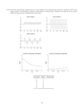
139. (b) Find the Fourier transform of g(t) convolved with itself.
F{g(t) ∗ g(t)} = ?
(c) Find the Fourier transform of g(t − 1) ∗ g(t − 2).
F{g(t − 1) ∗ g(t − 2)} = ?
(Use part (a) together with properties of the Fourier transform.)
(d) Find the Fourier transform of g(t) multiplied with itself.
F{g(t) · g(t)} = ?
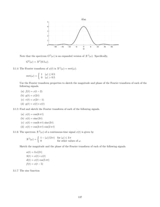
3.1.11 The signal x(t) is a cosine pulse,
x(t) = cos(10 π t) [u(t + 1) − u(t − 1)].
Find and make a rough sketch of its Fourier transform Xf
(ω). Also, make a sketch of x(t).
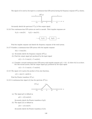
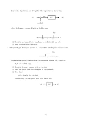
3.1.12 The signal x(t) has the spectrum Xf
(ω),
ω
−4π −2π 0 2π 4π
Xf
(ω)
1
The signal x(t) is used as the input to a continuous-time LTI system having the frequency response Hf
(ω),
ω
−4π −2π 0 2π 4π
Hf
(ω)
1
Accurately sketch the spectrum Y f
(ω) of the output signal.
3.1.13 Consider a continuous-time LTI system with the impulse response
h(t) = δ(t) − 2 sinc(2 t).
(a) Accurately sketch the frequency response Hf
(ω).
(b) Find the output signal y(t) produced by the input signal
x(t) = 3 + 4 sin(πt) + 5 cos(3πt).
3.1.14 Find the Fourier transform Xf
(ω) of the signal
x(t) = cos 5πt +
π
4
.
3.1.15 The signal x(t) has the spectrum Xf
(ω) shown.
ω
−4π −2π 0 2π 4π
Xf
(ω)
1
139

140. The signal x(t) is used as the input to a continuous-time LTI system having the frequency response Hf
(ω) shown.
ω
−4π −2π 0 2π 4π
Hf
(ω)1 1
Accurately sketch the spectrum Y f
(ω) of the output signal.
3.1.16 Two continuous-time LTI system are used in cascade. Their impulse responses are
h1(t) = sinc(3 t) h2(t) = sinc(5 t).
- h1(t) - h2(t) -
Find the impulse response and sketch the frequency response of the total system.
3.1.17 Consider a continuous-time LTI system with the impulse response
h(t) = 3 sinc(3 t).
(a) Accurately sketch the frequency response Hf
(ω).
(b) Find the output signal y(t) produced by the input signal
x(t) = 2 + 5 cos(πt) + 7 cos(4πt).
(c) Consider a second continuous-time LTI system with impulse response g(t) = h(t−2) where h(t) is as above.
For this second system, find the output signal y(t) produced by the input signal
x(t) = 2 + 5 cos(πt) + 7 cos(4πt).
3.1.18 The signal x(t) is given the product of two sine functions,
x(t) = sin(π t) · sin(2π t).
Find the Fourier transform Xf
(ω).
3.1.19 A continuous-time signal x(t) has the spectrum Xf
(ω),
ω
−4π −2π 0 2π 4π
Xf
(ω) 1
(a) The signal g(t) is defined as
g(t) = x(t) cos(4πt).
Accurately sketch the Fourier transform of g(t).
(b) The signal f(t) is defined as
f(t) = x(t) cos(πt).
Accurately sketch the Fourier transform of f(t).
140

141. 3.1.20 The signal x(t):
−6 −4 −2 0 2 4 6
0
0.5
1
1.5
2
t
x(t)
has the Fourier transform Xf
(ω):
−3π −2π −π 0 π 2π 3π
0
1
2
3
4
5
ω
X
f
(ω)
Accurately sketch the signal g(t) that has the spectrum Gf
(ω):
−3π −2π −π 0 π 2π 3π
0
1
2
3
4
5
ω
G
f
(ω)
Note that the spectrum Gf
(ω) is a sum of left- and right-shifted copies of Xf
(ω). Specifically,
Gf
(ω) = Xf
(ω − 2π) + Xf
(ω + 2π).
In your sketch of the signal g(t) indicate its zero-crossings. Show and explain your work.
3.1.21 The left-hand column below shows four continuous-time signals. The Fourier transform of each signal appears
in the right-hand column in mixed-up order. Match the signal to its Fourier transform.
Signal Fourier transform
1
2
3
4
141

142. −5 0 5
0
0.5
1
1.5
t
x(t)
#1
−5 0 5
−1
0
1
2
ω/π
Xf
(ω) C
−5 0 5
0
0.5
1
1.5
t
x(t)
#2
−5 0 5
0
2
4
ω/π
Xf
(ω)
D
−5 0 5
−0.5
0
0.5
1
1.5
t
x(t)
#3
−5 0 5
0
0.5
1
1.5
ω/π
Xf
(ω)
B
−5 0 5
−1
0
1
2
t
x(t)
#4
−5 0 5
0
0.5
1
1.5
ω/π
Xf
(ω)
A
142

143. 3.1.22 The ideal continuous-time high-pass filter has the frequency response
Hf
(ω) =



0, |ω| ≤ ωc
1, |ω| ωc.
Find the impulse response h(t).
3.1.23 The ideal continuous-time band-stop filter has the frequency response
Hf
(ω) =



1 |ω| ≤ ω1
0 ω1 |ω| ω2
1 |ω| ≥ ω2.
(a) Sketch Hf
(ω).
(b) What is the impulse response h(t) of the ideal band-stop filter?
(c) Describe how to implement the ideal band-stop filter using only lowpass and highpass filters.
3.1.24 The ideal continuous-time band-pass filter has the frequency response
Hf
(ω) =



0 |ω| ≤ ω1
1 ω1 |ω| ω2
0 |ω| ≥ ω2.
Describe how to implement the ideal band-pass using two ideal low-pass filters with different cut-off frequencies.
(Should a parallel or cascade structure be used?) Using that, find the impulse response h(t) of the ideal band-pass
filter.
3.1.25 The frequency response of a continuous-time LTI is given by
Hf
(ω) =



0 |ω| 2 π
1 |ω| ≥ 2 π
(This is an ideal high-pass filter.) Use the Fourier transform to find the output y(t) when the input x(t) is given
by
(a) x(t) = sinc(t) = sin(π t)
π t
(b) x(t) = sinc(3 t) = sin(3 π t)
3 π t
3.1.26 What is the Fourier transform of x(t)?
x(t) = cos(0.3 π t) · sin(0.1 π t)
Xf
(ω) = F{x(t)} = ?
3.1.27 A continuous-time LTI system has the impulse response
h(t) = δ(t) − 3 sinc(3t)
The input signal x(t) has the spectrum Xf
(ω) shown,
ω
−4π −3π −2π −π 0 π 2π 3π 4π
Xf
(ω)
2π
(1.5π)(1.5π)
(π)(π)
143

144. Find the output signal y(t).
3.1.28 A continuous-time LTI system has the impulse response
h(t) = 3 sinc(3t) − sinc(t).
The input signal x(t) has the spectrum Xf
(ω) shown,
ω
−4π −3π −2π −π 0 π 2π 3π 4π
Xf
(ω)
2π
(1.5π)(1.5π)
(π)(π)
Find the output signal y(t). (Hint: first find Hf
(ω).)
3.2 Fourier Series
3.2.1 Consider the signal
x(t) = cos(10 π t)
(a) Write the Fourier series expansion of x(t).
(b) Sketch the line spectrum of x(t).
3.2.2 Consider the signal
x(t) = cos(12 π t) cos(8 π t).
(a) Write the Fourier series expansion of x(t).
(b) Sketch the line spectrum of x(t).
3.2.3 Find the Fourier series coefficients c(k) for the periodic signal
x(t) = | cos(t)|.
Using Matlab, plot the truncated Fourier series:
xN (t) =
N
k=−N
ck ejkωot
for N = 10. Does it resemble the signal x(t)?
3.2.4 The periodic signal x(t) is given by
x(t) = | sin(t)|.
(a) Sketch the signal x(t). What is its period?
(b) Find the Fourier series coefficients of x(t). Simplify!
(c) Is x(t) band-limited?
3.2.5 Find the Fourier series coefficients c(k) for the periodic triangular pulse shown below.
144

145. x(t)
-
−5 −4 −3 −2 −1 0 1 2 3 4 5
1
· · ·
d
dd
d
dd
d
dd
d
dd
d
dd
· · ·
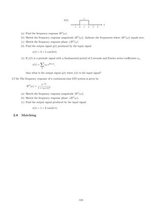
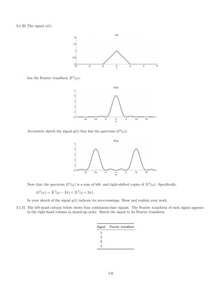
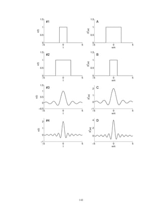
3.2.6 Fourier series:
3.2.7 The signal x(t) is
x(t) = [cos(π t)]2
sin(πt).
(a) Find its Fourier transform Xf
(ω).
(b) Is x(t) periodic? If so, determine the Fourier series coefficients of x(t).
3.2.8 The signal x(t), which is periodic with period T = 1/4, has the Fourier series coefficients
ck =
1
1 + k2
.
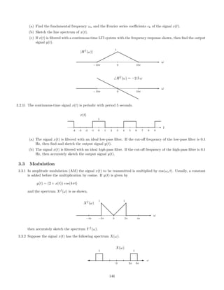
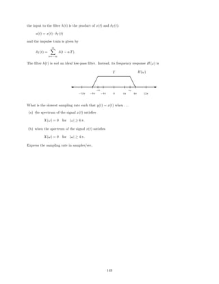
The signal is filtered with an ideal lowpass filter with cut-off frequency of fc = 5.2 Hz. What is the output of the
filter?
Simplify your answer so it does not contain any complex numbers. Note: ω = 2 π f converts from physical
frequency to angular frequency.
3.2.9 Consider the signal
x(t) = |0.5 + cos(4πt)|
The signal is filtered with an ideal bandpass filter that only passes frequencies between 2.5 Hz and 3.5 Hz.
Hf
(ω) =



0 |ω| 5 π
1 5 π ≤ |ω| ≤ 7 π
0 |ω| 7 π
(a) Sketch the input signal x(t).
(b) Find and sketch the output signal y(t). Hint: Use the Fourier series, but do not compute the Fourier series
of x(t).
3.2.10 A continuous-time signal x(t) is given by
x(t) = 2 cos(6πt) + 3 cos(8πt).
145

146. (a) Find the fundamental frequency ωo and the Fourier series coefficients ck of the signal x(t).
(b) Sketch the line spectrum of x(t).
(c) If x(t) is filtered with a continuous-time LTI system with the frequency response shown, then find the output
signal y(t).
ω
−10π 0 10π
|Hf
(ω)|
1
ω
−10π 0 10π
∠Hf
(ω) = −2.5 ω
3.2.11 The continuous-time signal x(t) is periodic with period 5 seconds.
1
-4 -3 -2 -1 0 1 2 3 4 5 6 7 8 9
t
x(t)
(a) The signal x(t) is filtered with an ideal low-pass filter. If the cut-off frequency of the low-pass filter is 0.1
Hz, then find and sketch the output signal y(t).
(b) The signal x(t) is filtered with an ideal high-pass filter. If the cut-off frequency of the high-pass filter is 0.1
Hz, then accurately sketch the output signal y(t).
3.3 Modulation
3.3.1 In amplitude modulation (AM) the signal x(t) to be transmitted is multiplied by cos(ωo t). Usually, a constant
is added before the multiplication by cosine. If y(t) is given by
y(t) = (2 + x(t)) cos(4πt)
and the spectrum Xf
(ω) is as shown,
ω
−4π −2π 0 2π 4π
Xf
(ω)
1 1
then accurately sketch the spectrum Y f
(ω).
3.3.2 Suppose the signal x(t) has the following spectrum X(ω).
X(ω)
E'
0
1 1
2π 3π
ω
146

147. Suppose the signal x(t) is sent through the following continuous-time system.
x(t) E g× Ea(t)
h(t) E y(t)
T
cos(3 π t)
where the frequency response H(ω) is an ideal low-pass,
E
H(ω)
'
−2 π 0
1
2 π
ω
(a) Sketch the spectrums (Fourier transforms) of cos(3 π t), a(t), and y(t).
(b) Is the total system an LTI system?
3.3.3 Suppose h(t) is the impulse response of a lowpass filter with frequency response shown.
H(ω)
-
−π 0
1
π
ω
Suppose a new system is constructed so that its impulse response h2(t) is given by
h2(t) = 2 cos(6 π t) · h(t).
(a) Sketch the frequency response of the new system.
(b) Is the new system a low-pass, band-pass, or high-pass filter?
(c) If the signal
x(t) = 2 cos (3π t) + 4 sin (6π t)
is sent through the new system, what is the output y(t)?
x(t) E h2(t) E y(t)
147

148. 4 The Sampling Theorem
4.0.1 The Fourier transform of a signal x(t) satisfies
X(ω) = 0 for |ω| ≥ 8 π.
What is the maximum sampling period T such that x(t) can be recovered from the samples x(nT)?
4.0.2 For the following continuous-time system
x(t) E g× Ea(t)
h(t) E y(t)
T
δs(t)
the input to the filter h(t) is the product of x(t) and δs(t):
a(t) = x(t) · δs(t)
and the impulse train is given by
δs(t) =
∞
n=−∞
δ(t − n Ts)
where the sampling period is
Ts =
2
3
.
The frequency response H(ω) is an ideal low-pass,
−2 π 0
1
2 π
ω
H(ω)
Suppose the input signal is
x(t) = 4 cos(6 π t).
(a) Sketch the spectrums (Fourier transforms) of x(t), δs(t), a(t), and y(t).
(b) Find and sketch a(t) and y(t).
(c) Does y(t) = x(t)? Does this contradict the sampling theorem? Explain.
4.0.3 For the following continuous-time system
x(t) E g× Ea(t)
h(t) E y(t)
T
δT (t)
148

149. the input to the filter h(t) is the product of x(t) and δT (t):
a(t) = x(t) · δT (t)
and the impulse train is given by
δT (t) =
∞
n=−∞
δ(t − n T).
The filter h(t) is not an ideal low-pass filter. Instead, its frequency response H(ω) is
H(ω)T
−12π −8π −4π 0 4π 8π 12π
−6π 6π
' ¡
¡
¡ e
e
e E
What is the slowest sampling rate such that y(t) = x(t) when . . .
(a) the spectrum of the signal x(t) satisfies
X(ω) = 0 for |ω| ≥ 6 π.
(b) when the spectrum of the signal x(t) satisfies
X(ω) = 0 for |ω| ≥ 4 π.
Express the sampling rate in samples/sec.
149