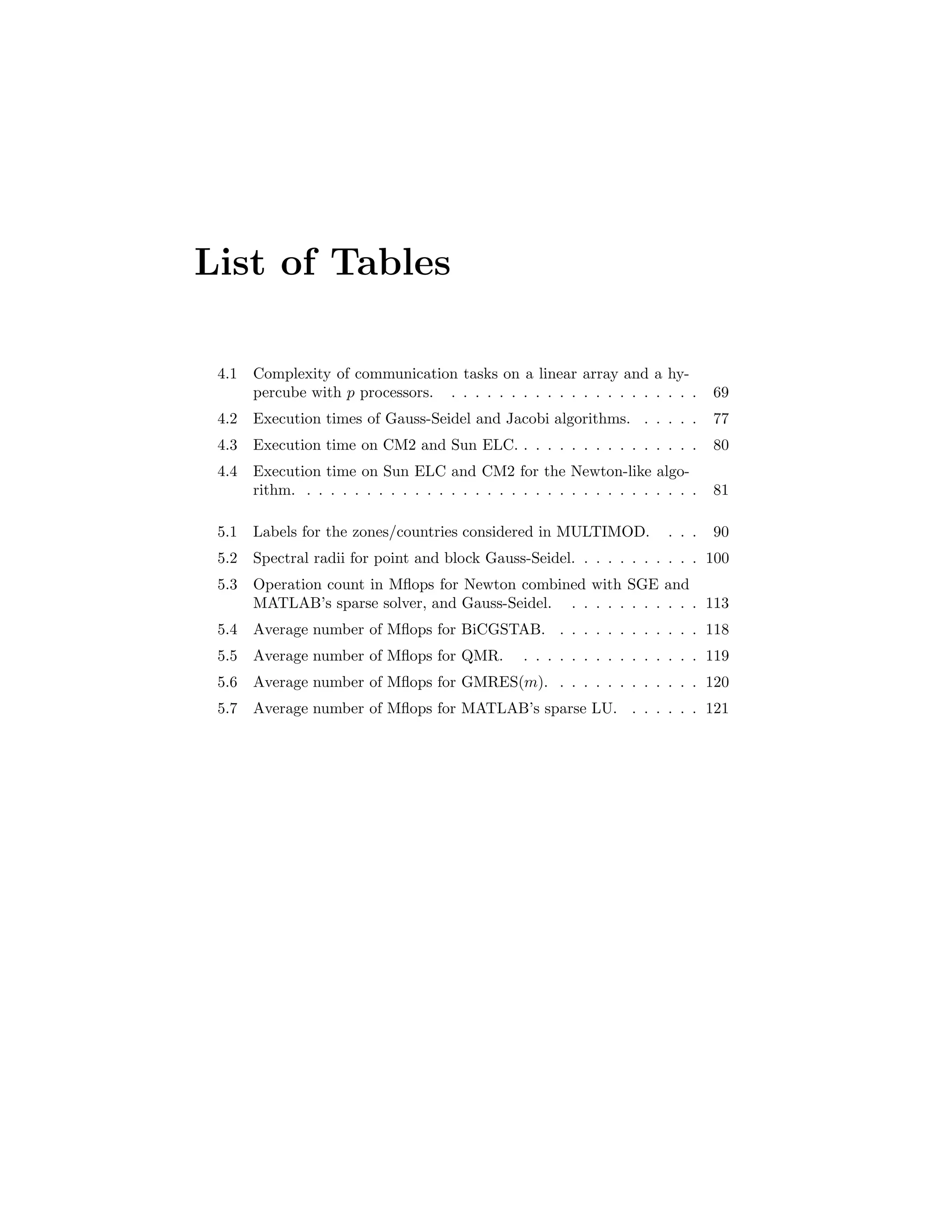
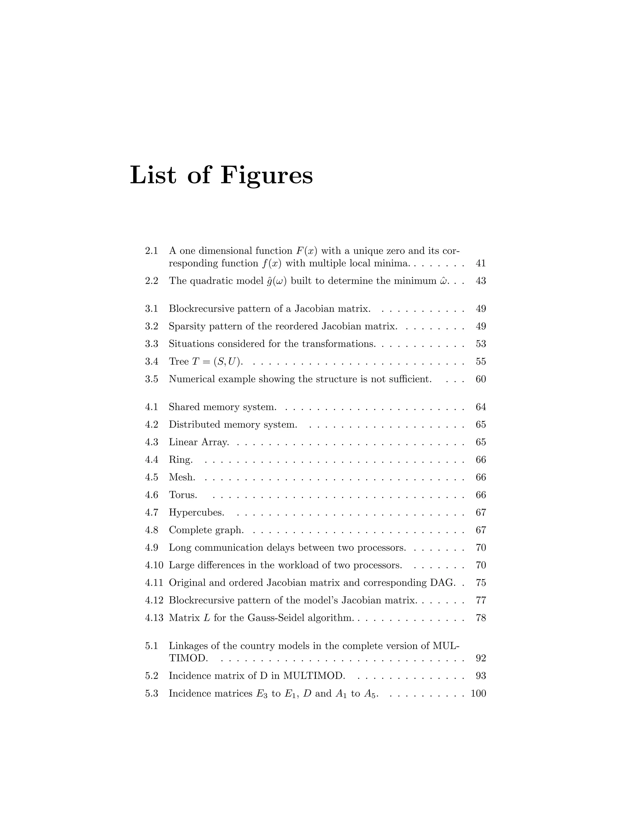
Download to read offline


![Chapter 2
A Review of Solution
Techniques
This chapter reviews classic and well implemented solution techniques for linear
and nonlinear systems. First, we discuss direct and iterative methods for linear
systems. Some of these methods are part of the fundamental building blocks
for many techniques for solving nonlinear systems presented later. The topic
has been extensively studied and many methods have been analyzed in scientific
computing literature, see e.g. Golub and Van Loan [56], Gill et al. [47], Barrett
et al. [8] and Hageman and Young [60].
Second, the nonlinear case is addressed essentially presenting methods based on
Newton iterations.
First, direct methods for solving linear systems of equations are displayed. The
first section presents the LU factorization—or Gaussian elimination technique—
is presented and the second section describes, an orthogonalization decompo-
sition leading to the QR factorization. The case of dense and sparse systems
are then addressed. Other direct methods also exist, such as the Singular Value
Decomposition (SVD) which can be used to solve linear systems. Even though
this can constitute an interesting and useful approach we do not resort to it
here.
Section 2.4 introduces stationary iterative methods such as Jacobi, Gauss-Seidel,
SOR techniques and their convergence characteristics.
Nonstationary iterative methods—such as the conjugate gradient, general min-
imal residual and biconjugate gradient, for instance—a class of more recently
developed techniques constitute the topic of Section 2.5.
Section 2.10 presents nonlinear first-order methods that are quite popular in
macroeconometric modeling. The topic of Section 2.11 is an alternative ap-
proach to the solution of a system of nonlinear equations: a minimization of the
residuals norm.
To overcome the nonconvergent behavior of the Newton method in some circum-
stances, two globally convergent modifications are introduced in Section 2.12.](https://image.slidesharecdn.com/c12cdca8-ad4d-451a-b4fb-6c6bd72ac4d1-161015164104/75/t-12-2048.jpg)
![2.1 LU Factorization 5
Finally, we discuss stopping criteria and scaling.
2.1 LU Factorization
For a linear model, finding a vector of solutions amounts to solving for x a
system written in matrix form
Ax = b , (2.1)
where A is a n × n real matrix and b a n × 1 real vector.
System (2.1) can be solved by the Gaussian elimination method which is a
widely used algorithm and here, we present its application for a dense matrix
A with no particular structure.
The basic idea of Gaussian elimination is to transform the original system into
an equivalent triangular system. Then, we can easily find the solution of such
a system. The method is based on the fact that replacing an equation by a
linear combination of the others leaves the solution unchanged. First, this idea
is applied to get an upper triangular equivalent system. This stage is called the
forward elimination of the system. Then, the solution is found by solving the
equations in reverse order. This is the back substitution phase.
To describe the process with matrix algebra, we need to define a transformation
that will take care of zeroing the elements below the diagonal in a column of
matrix A. Let x ∈ Rn
be a column vector with xk = 0. We can define
τ(k)
= [0 . . . 0 τ
(k)
k+1 . . . τ(k)
n ] with τ
(k)
i = xi/xk for i = k + 1, . . . , n .
Then, the matrix Mk = I −τ(k)
ek with ek being the k-th standard vector of Rn
,
represents a Gauss transformation. The vector τ(k)
is called a Gauss vector. By
applying Mk to x, we check that we get
Mkx =
1 · · · 0 0 · · · 0
...
...
...
...
...
0 · · · 1 0 · · · 0
0 · · · −τ
(k)
k+1 1 · · · 0
...
...
...
...
...
0 · · · −τ
(k)
n 0 · · · 1
x1
...
xk
xk+1
...
xn
=
x1
...
xk
0
...
0
.
Practically, applying such a transformation is carried out without explicitly
building Mk or resorting to matrix multiplications. For example, in order to
multiply Mk by a matrix C of size n × r, we only need to perform an outer
product and a matrix subtraction:
MkC = (I − τ(k)
ek)C = C − τ(k)
(ekC) . (2.2)
The product ekC selects the k-th row of C, and the outer product τ(k)
(ekC) is
subtracted from C. However, only the rows from k + 1 to n of C have to be
updated as the first k elements in τ(k)
are zeros. We denote by A(k)
the matrix
Mk · · · M1A, i.e. the matrix A after the k-th elimination step.](https://image.slidesharecdn.com/c12cdca8-ad4d-451a-b4fb-6c6bd72ac4d1-161015164104/75/t-13-2048.jpg)
![2.1 LU Factorization 6
To triangularize the system, we need to apply n − 1 Gauss transformations,
provided that the Gauss vector can be found. This is true if all the divisors
a
(k)
kk —called pivots—used to build τ(k)
for k = 1, . . . , n are different from zero.
If for a real n×n matrix A the process of zeroing the elements below the diagonal
is successful, we have
Mn−1Mn−2 · · · M1A = U ,
where U is a n × n upper triangular matrix. Using the Sherman-Morrison-
Woodbury formula, we can easily find that if Mk = I − τ(k)
ek then M−1
k =
I + τ(k)
ek and so defining L = M−1
1 M−1
2 · · · M−1
n−1 we can write
A = LU .
As each matrix Mk is unit lower triangular, each M−1
k also has this property;
therefore, L is unit lower triangular too. By developing the product defining L,
we have
L = (I + τ(1)
e1)(I + τ(2)
e2) · · · (I + τ(n−1)
en−1) = I +
n−1
k=1
τ(k)
ek .
So L contains ones on the main diagonal and the vector τ(k)
in the k-th column
below the diagonal for k = 1, . . . , n − 1 and we have
L =
1
τ
(1)
1 1
τ
(1)
2 τ
(2)
1 1
...
...
...
τ
(1)
n−1 τ
(2)
n−2 · · · τ
(n−1)
1 1
.
By applying the Gaussian elimination to A we found a factorization of A into a
unit lower triangular matrix L and an upper triangular matrix U. The existence
and uniqueness conditions as well as the result are summarized in the following
theorem.
Theorem 1 A ∈ Rn×n
has an LU factorization if the determinants of the first
n − 1 principal minors are different from 0. If the LU factorization exists and
A is nonsingular, then the LU factorization is unique and det(A) = u11 · · · unn.
The proof of this theorem can be found for instance in Golub and Van Loan [56,
p. 96]. Once the factorization has been found, we obtain the solution for the
system Ax = b, by first solving Ly = b by forward substitution and then solving
Ux = y by back substitution.
Forward substitution for a unit lower triangular matrix is easy to perform. The
first equation gives y1 = b1 because L contains ones on the diagonal. Substitut-
ing y1 in the second equation gives y2. Continuing thus, the triangular system
Ly = b is solved by substituting all the known yj to get the next one.
Back substitution works similarly, but we start with xn since U is upper trian-
gular. Proceeding backwards, we get xi by replacing all the known xj (j > i)
in the i-th equation of Ux = y.](https://image.slidesharecdn.com/c12cdca8-ad4d-451a-b4fb-6c6bd72ac4d1-161015164104/75/t-14-2048.jpg)
![2.1 LU Factorization 7
2.1.1 Pivoting
As described above, the Gaussian elimination breaks down when a pivot is equal
to zero. In such a situation, a simple exchange of the equations leading to a
nonzero pivot may get us round the problem. However, the condition that all
the pivots have to be different than zero does not suffice to ensure a numerically
reliable result. Moreover at this stage, the Gaussian elimination method, is
still numerically unstable. This means that because of cancellation errors, the
process described can lead to catastrophic results. The problem lies in the size
of the elements of the Gauss vector τ. If they are too large compared to the
elements from which they are subtracted in Equation (2.2), rounding errors may
be magnified thus destroying the numerical accuracy of the computation.
To overcome this difficulty a good strategy is to exchange the rows of the matrix
during the process of elimination to ensure that the elements of τ will always
be smaller or equal to one in magnitude. This is achieved by choosing the
permutation of the rows so that
|a
(k)
kk | = max
i>k
|a
(k)
ik | . (2.3)
Such an exchange strategy is called partial pivoting and can be formalized in
matrix language as follows.
Let Pi be a permutation matrix of order n, i.e. the identity matrix with its rows
reordered. To ensure that no element in τ is larger than one in absolute value,
we must permute the rows of A before applying the Gauss transformation. This
is applied at each step of the Gaussian elimination process, which leads to the
following theorem:
Theorem 2 If Gaussian elimination with partial pivoting is used to compute
the upper triangularization
Mn−1Pn−1 · · · M1P1A = U ,
then PA = LU where P = Pn−1 · · · P1 and L is a unit lower triangular matrix
with | ij| ≤ 1.
Thus, when solving a linear system Ax = b, we first compute the vector y =
Mn−1Pn−1 · · · M1P1b and then solve Ux = y by back substitution. This method
is much more stable and it is very unlikely to find catastrophic cancellation
problems. The proof of Theorem 2 is given in Golub and Van Loan [56, p. 112].
Going one step further would imply permuting not only the rows but also the
columns of A so that in the k-th step of the Gaussian elimination the largest
element of the submatrix to be transformed is used as pivot. This strategy is
called complete pivoting. However, applying complete pivoting is costly because
one needs to search for the largest element in a matrix instead of a vector at
each elimination step. This overhead does not justify the gain one may obtain
in the stability of the method in practice. Therefore, the algorithm of choice
for solving Ax = b, when A has no particular structure, is Gaussian elimination
with partial pivoting.](https://image.slidesharecdn.com/c12cdca8-ad4d-451a-b4fb-6c6bd72ac4d1-161015164104/75/t-15-2048.jpg)
![2.2 QR Factorization 8
2.1.2 Computational Complexity
The number of elementary arithmetic operations (flops) for the Gaussian elim-
ination is 2
3 n3
− 1
2 n2
− 1
6 n and therefore this methods is O(n3
).
2.1.3 Practical Implementation
In the case where one is only interested in the solution vector, it is not necessary
to explicitly build matrix L. It is possible to directly compute the y vector
(solution of Ly = b) while transforming matrix A into an upper triangular
matrix U.
Despite the fact that Gaussian elimination seems to be easy to code, it is cer-
tainly not advisable to write our own code. A judicious choice is to rely on
carefully tested software as the routines in the LAPACK library. These routines
are publicly available on NETLIB1
and are also used by the software MATLAB2
which is our main computing environment for the experiments we carried out.
2.2 QR Factorization
The QR factorization is an orthogonalization method that can be applied to
square or rectangular matrices. Usually this is a key algorithm for computing
eigenvalues or least-squares solutions and it is less applied to find the solution
of a square linear system. Nevertheless, there are at least 3 reasons (see Golub
and Van Loan [56]) why orthogonalization methods, such as QR, might be
considered:
• The orthogonal methods have guaranteed numerical stability which is not
the case for Gaussian elimination.
• In case of ill-conditioning, orthogonal methods give an added measure of
reliability.
• The flop count tends to exaggerate the Gaussian elimination advantage.3
(Particularly for parallel computers, memory traffic and other overheads
tend to reduce this advantage.)
Another advantage that might favor the QR factorization is the possibility of up-
dating the factors Q and R corresponding to a rank one modification of matrix
A in O(n2
) operations. This is also possible for the LU factorization; however,
1NETLIB can be accessed through the World Wide Web at http://www.netlib.org/
and collects mathematical software, articles and databases useful for the scientific com-
munity. In Europe the URL is http://www.netlib.no/netlib/master/readme.html or
http://elib.zib-berlin.de/netlib/master/readme.html .
2MATLAB High Performance Numeric Computation and Visualization Software is a prod-
uct and registered trademark of The MathWorks, Inc., Cochituate Place, 24 Prime Park Way,
Natick MA 01760, USA. URL: http://www.mathworks.com/ .
3In the application discussed in Section 4.2.2 we used the QR factorization available in the
libraries of the CM2 parallel computer.](https://image.slidesharecdn.com/c12cdca8-ad4d-451a-b4fb-6c6bd72ac4d1-161015164104/75/t-16-2048.jpg)
![2.2 QR Factorization 9
the implementation is much simpler with QR, see Gill et al. [47]. Updating tech-
niques will prove particularly useful in the quasi-Newton algorithm presented
in Section 2.9.
These reasons suggest that QR probably are, especially on parallel devices, a
possible alternative to LU to solve square systems. The QR factorization can
be applied to any rectangular matrix, but we will focus on the case of a n × n
real matrix A.
The goal is to apply to A successive orthogonal transformation matrices Hi,
i = 1, 2, . . . , r to get an upper triangular matrix R, i.e.
Hr · · · H1A = R .
The orthogonal transformations presented in the literature are usually based
upon Givens rotations or Householder reflections. This latter choice leads to
algorithms involving less arithmetic operations and is therefore presented in the
following.
A Householder transformation is a matrix of the form
H = I − 2ww with w w = 1 .
Such a matrix is symmetric, orthogonal and its determinant is −1. Geometri-
cally, this matrix represents a reflection with respect to the hyperplane defined
by {x|w x = 0}. By properly choosing the reflection plane, it is possible to zero
particular elements in a vector.
Let us partition our matrix A in n column vectors [a1 · · · an]. We first look for
a matrix H1 such as all the elements of H1a1 except the first one are zeros. We
define
s1 = −sign(a11) a1
µ1 = (2s2
1 − 2a11s1)−1/2
u1 = [(a11 − s1) a21 · · · an1]
w1 = µ1u1 .
Actually the sign of s1 is free, but it is chosen to avoid catastrophic cancellation
that may otherwise appear in computing µ1. As w1w1 = 1, we can let H1 =
I − 2w1w1 and verify that H1a1 = [s1 0 · · · 0] .
Computationally, it is more efficient to calculate the product H1A in the fol-
lowing manner
H1A = A − 2w1w1A
= A − 2w1 w1a1 w1a2 · · · w1am
so the i-th column of H1A is ai − 2(w1ai)w1 = ai − (c1 u1ai)w1 and c1 = 2µ2
1 =
(s2
1 − s1a11)−1
.
We continue this process in a similar way on a matrix A where we have removed
the first row and column. The vectors w2 and u2 will now be of dimension
(n − 1) × 1 but we can complete them with zeros to build
H2 = I −
0
w2
0 w2 .](https://image.slidesharecdn.com/c12cdca8-ad4d-451a-b4fb-6c6bd72ac4d1-161015164104/75/t-17-2048.jpg)
![2.3 Direct Methods for Sparse Matrices 10
After n − 1 steps, we have Hn−1 · · · H2H1A = R. As all the matrices Hi are
orthogonal, their product is orthogonal too and we get
A = QR ,
with Q = (Hn−1 · · · H1) = H1 · · · Hn−1. In practice, one will neither form the
vectors wi nor calculate the Q matrix as all the information is contained in the
ui vectors and the si scalars for i = 1, . . . , n.
The possibility to choose the sign of s1 such that there never is a subtraction
in the computation of µ1 is the key for the good numerical behavior of the QR
factorization. We notice that the computation of u1 also involves a subtraction.
It is possible to permute the column with the largest sum of squares below row
i − 1 into column i during the i-th step in order to minimize the risk of digit
cancellation. This then leads to a factorization
PA = QR ,
where P is a permutation matrix.
Using this factorization of matrix A, it is easy to find a solution for the system
Ax = b. We first compute y = Q b and then solve Rx = y by back substitution.
2.2.1 Computational Complexity
The computational complexity of the QR algorithm for a square matrix of order
n is 4
3 n3
+ O(n2
). Hence the method is of O(n3
) complexity.
2.2.2 Practical Implementation
Again as for the LU decomposition, the explicit computation of matrix Q is not
necessary as we may build vector y during the triangularization process. Only
the back substitution phase is needed to get the solution of the linear system
Ax = b.
As has already been mentioned, the routines for computing a QR factoriza-
tion (or solving a system via QR) are readily available in LAPACK and are
implemented in MATLAB.
2.3 Direct Methods for Sparse Matrices
In many cases, matrix A of the linear system contains numerous zero entries.
This is particularly true for linear systems derived from large macroeconometric
models. Such a situation may be exploited in order to organize the computations
in a way that involves only the nonzero elements. These techniques are known as
sparse direct methods (see e.g. Duff et al. [30]) and crucial for efficient solution
of linear systems in a wide class of practical applications.](https://image.slidesharecdn.com/c12cdca8-ad4d-451a-b4fb-6c6bd72ac4d1-161015164104/75/t-18-2048.jpg)

![2.3 Direct Methods for Sparse Matrices 12
List of successors (Collection of Sparse Vectors)
With this storage scheme, the sparse matrix A is stored as the concatenation
of the sparse vectors representing its columns. Each sparse vector consists of a
real array containing the nonzero entries and an integer array of corresponding
row indices. A second integer array gives the locations in the other arrays of
the first element in each column.
For our matrix A, this representation is
index 1 2 3 4 5 6
h 1 2 4 6 9 11
index 1 2 3 4 5 6 7 8 9 10
4 1 2 3 5 2 4 5 1 3
x 3.1 −2 5 1.7 1.2 7 −0.2 −3 0.5 6
The integer array h contains the addresses of the list of row elements in and
x. For instance, the nonzero entries in column 4 of A are stored at positions
h(4) = 6 to h(5)−1 = 9−1 = 8 in x. Thus, the entries are x(6) = 7, x(7) = −0.2
and x(8) = −3. The row indices are given by the same locations in array , i.e.
(6) = 2, (7) = 4 and (8) = 5.
MATLAB mainly uses this data structure to store its sparse matrices, see Gilbert
et al. [44]. The main advantage is that columns can be easily accessed, which
is of very important for numerical linear algebra algorithms. The disadvantage
of such a representation is the difficulty of inserting new entries. This arises for
instance when adding a row to another.
Linked List
The third alternative that is widely used for storing sparse matrices is the linked
list. Its particularity is that we define a pointer (named head) to the first entry
and each entry is associated to a pointer pointing to the next entry or to the
null pointer (named 0) for the last entry. If the matrix is stored by columns,
we start a new linked list for each column and therefore we have as many head
pointers as there are columns. Each entry is composed of two pieces: the row
index and the value of the entry itself.
This is represented by the picture:
head 1 4 3.1 0
head 5 1 0.5 3 6 0
E
E E
...
•
The structure can be implemented as before with arrays and we get](https://image.slidesharecdn.com/c12cdca8-ad4d-451a-b4fb-6c6bd72ac4d1-161015164104/75/t-20-2048.jpg)
![2.3 Direct Methods for Sparse Matrices 13
index 1 2 3 4 5
head 4 5 9 1 7
index 1 2 3 4 5 6 7 8 9 10
row 2 4 5 4 1 2 1 3 3 5
entry 7 −0.2 −3 3.1 −2 5 0.5 6 1.7 1.2
link 2 3 0 0 6 0 8 0 10 0
For instance, to retrieve the elements of column 3, we begin to read head(3)=9.
Then row(9)=3 gives the row index, the entry value is entry(9)=1.7 and the
pointer link(9)=10 gives the next index address. The values row(10)=5, en-
try(10)=1.2 and link(10)=0 indicate that the element 1.2 is at row number 5
and is the last entry of the column.
The obvious advantage is the ease with which elements can be inserted and
deleted: the pointers are simply updated to take care of the modification. This
data structure is close to the list of successors representation, but does not
necessitate contiguous storage locations for the entries of a same column.
In practice it is often necessary to switch from one representation to another.
We can also note that the linked list and the list of successors can similarly be
defined row-wise rather than column wise.
2.3.2 Fill-in in Sparse LU
Given a storage scheme, one could think of executing a Gaussian elimination as
described in Section 2.1. However, by doing so we may discover that the sparsity
of our initial matrix A is lost and we may obtain relatively dense matrices L
and U.
Indeed, depending on the choice of the pivots, the number of entries in L and
U may vary. From Equation (2.2), we see that at step k of the Gaussian elimi-
nation algorithm, we subtract two matrices in order to zero the elements below
the diagonal of the k-th column. Depending on the Gauss vector τ(k)
, matrix
τ(k)
ekC may contain nonzero elements which do not exist in matrix C. This
creation of new elements is called fill-in.
A crucial problem is then to minimize the fill-in as the number of operations is
proportional to the density of the submatrix to be triangularized. Furthermore,
a dense matrix U will result in an expensive back substitution phase.
A minimum fill-in may however conflict with the pivoting strategy, i.e. the
pivot chosen to minimize the fill-in may not correspond to the element with
maximum magnitude among the elements below the k-th diagonal as defined
by Equation (2.3). A common tradeoff to limit the loss of numerical stability
of the sparse Gaussian elimination is to accept a pivot element satisfying the
following threshold inequality
|a
(k)
kk | ≥ u max
i>k
|a
(k)
ik | ,
where u is the threshold parameter and belongs to (0, 1]. A choice for u suggested
by Duff, Erisman and Reid [30] is u = 0.1 . This parameter heavily influences
the fill-in and hence the complexity of the method.](https://image.slidesharecdn.com/c12cdca8-ad4d-451a-b4fb-6c6bd72ac4d1-161015164104/75/t-21-2048.jpg)
![2.4 Stationary Iterative Methods 14
2.3.3 Computational Complexity
It is not easy to establish an exact operation count for the sparse LU. The count
depends on the particular structure of matrix A and on the chosen pivoting
strategy. For a good implementation, we may expect a complexity of O(c2
n)
where c is the average number of elements in a row and n is the order of matrix
A.
2.3.4 Practical Implementation
A widely used code for the direct solution of sparse linear systems is the Harwell
MA28 code available on NETLIB, see Duff [29]. A new version called MA48 is
presented in Duff and Reid [31].
The software MATLAB has its own implementation using partial pivoting and
minimum-degree ordering for the columns to reduce fill-in, see Gilbert et al. [44]
and Gilbert and Peierls [45].
Other direct sparse solvers are also available through NETLIB (e.g. Y12MA,
UMFPACK, SuperLU, SPARSE).
2.4 Stationary Iterative Methods
Iterative methods form an important class of solution techniques for solving
large systems of equations. They can be an interesting alternative to direct
methods because they take into account the sparsity of the system and are
moreover easy to implement.
Iterative methods may be divided into two classes: stationary and nonstationary.
The former rely on invariant information from an iteration to another, whereas
the latter modify their search by using the results of previous iterations.
In this section, we present stationary iterative methods such as Jacobi, Gauss-
Seidel and SOR techniques.
The solution x∗
of the system Ax = b can be approximated by replacing A by
a simpler nonsingular matrix M and by rewriting the systems as,
Mx = (M − A)x + b .
In order to solve this equivalent system, we may use the following recurrence
formula from a chosen starting point x0,
Mx(k+1)
= (M − A)x(k)
+ b , k = 0, 1, 2, . . . . (2.4)
At each step k the system (2.4) has to be solved, but this task can be easy
according to the choice of M.
The convergence of the iterates to the solution is not guaranteed. However, if
the sequence of iterates {x(k)
}k=0,1,2,... converges to a limit x(∞)
, then we have
x(∞)
= x∗
, since relation (2.4) becomes Mx(∞)
= (M − A)x(∞)
+ b, that is
Ax(∞)
= b.](https://image.slidesharecdn.com/c12cdca8-ad4d-451a-b4fb-6c6bd72ac4d1-161015164104/75/t-22-2048.jpg)

![2.4 Stationary Iterative Methods 16
This process amounts to using M = L + D and leads to the formula
(L + D)x(k+1)
= −Ux(k)
+ b ,
or to the following algorithm:
Algorithm 2 Gauss-Seidel Method
Given a starting point x(0)
∈ Rn
for k = 0, 1, 2, . . . until convergence
for i = 1, . . . , n
x
(k+1)
i = (bi −
j<i
aijx
(k+1)
i ) −
j>i
aij x
(k)
i )/aii
end
end
The matrix formulation of the iterations is useful for theoretical purposes, but
the actual computation will generally be implemented component-wise as in
Algorithm 1 and Algorithm 2.
2.4.3 Successive Overrelaxation Method
A third useful technique called SOR for Successive Overrelaxation method is
very closely related to the Gauss-Seidel method. The update is computed as an
extrapolation of the Gauss-Seidel step as follows: let x
(k+1)
GS denote the (k + 1)
iterate for the GS method; the new iterates can then be written as in the next
algorithm.
Algorithm 3 Successive Overrelaxation Method
Given a starting point x(0)
∈ Rn
for k = 0, 1, 2, . . . until convergence
Compute x
(k+1)
GS by Algorithm 2
for i=1,. . . ,n
x
(k+1)
i = x
(k)
i + ω(x
(k+1)
GS,i − x
(k)
i )
end
end
The scalar ω is called the relaxation parameter and its optimal value, in order to
achieve the fastest convergence, depends on the characteristics of the problem
in question. A necessary condition for the method to converge is that ω lies in
the interval (0, 2]. When ω < 1, the GS step is dampened and this is sometimes
referred to as under-relaxation.
In matrix form, the SOR iteration is defined by
(ωL + D)x(k+1)
= ((1 − ω)D − ωU)x(k)
+ ωb , k = 0, 1, 2, . . . . (2.5)
When ω is unity, the SOR method collapses to GS.](https://image.slidesharecdn.com/c12cdca8-ad4d-451a-b4fb-6c6bd72ac4d1-161015164104/75/t-24-2048.jpg)
![2.4 Stationary Iterative Methods 17
2.4.4 Fast Gauss-Seidel Method
The idea of extrapolating the step size to improve the speed of convergence
can also be applied to SOR iterates and gives rise to the Fast Gauss-Seidel
method (FGS) or Accelerated Over Relaxation method, see Hughes Hallett [68]
and Hadjidimos [59].
Let us denote by x
(k+1)
SOR the (k + 1) iterate obtained by Equation (3); then the
FGS iterates are defined by
Algorithm 4 FGS Method
Given a starting point x(0)
∈ Rn
for k = 0, 1, 2, . . . until convergence
Compute x
(k+1)
SOR by Algorithm 3
for i = 1, . . . , n
x
(k+1)
i = x
(k)
i + γ(x
(k+1)
SOR,i − x
(k)
i )
end
end
This method may be seen as a second-order method, since it uses a SOR iterate
as an intermediate step to compute its next guess, and that the SOR already
uses the information from a GS step. It is easy to see that when γ = 1, we find
the SOR method.
Like ω in the SOR part, the choice of the value for γ is not straightforward.
For some problems, the optimal choice of ω can be explicitly found (this is dis-
cussed in Hageman and Young [60]). However, it cannot be determined a priori
for general matrices. There is no way of computing the optimal value for γ
cheaply and some authors (e.g. Hughes Hallett [69], Yeyios [103]) offered ap-
proximations of γ. However, numerical tests produced variable outcomes: some-
times the approximation gave good convergence rates, sometimes poor ones, see
Hughes-Hallett [69]. As for the ω parameter, the value of γ is usually chosen by
experimentation on the characteristics of system at stake.
2.4.5 Block Iterative Methods
Certain problems can naturally be decomposed into a set of subproblems with
more or less tight linkages.4
In economic analysis, this is particularly true for
multi-country macroeconometric models where the different country models are
linked together by a relatively small number of trade relations for example (see
Faust and Tryon [35]). Another such situation is the case of disaggregated
multi-sectorial models where the links between the sectors are relatively weak.
In other problems where such a decomposition does not follow from the con-
struction of the system, one may resort to a partition where the subsystems are
easier to solve.
A block iterative method is then a technique where one iterates over the sub-
systems. The technique to solve the subsystem is free and not relevant for the
4The original problem is supposed to be indecomposable in the sense described in Sec-
tion 3.1.](https://image.slidesharecdn.com/c12cdca8-ad4d-451a-b4fb-6c6bd72ac4d1-161015164104/75/t-25-2048.jpg)
![2.4 Stationary Iterative Methods 19
Algorithm 6 Block Gauss-Seidel method (BGS)
Given a starting point x(0)
∈ Rn
for k = 0, 1, 2, . . . until convergence
Solve for y
(k+1)
i :
Aii y
(k+1)
i = bi −
i−1
j=1
Aij y
(k+1)
j −
N
j=i+1
Aij y
(k)
j , i = 1, 2, . . . , N
end
Similarly to the presentation in Section 2.4.3, the SOR option can also be applied
as follows:
Algorithm 7 Block successive over relaxation method (BSOR)
Given a starting point x(0)
∈ Rn
for k = 0, 1, 2, . . . until convergence
Solve for y
(k+1)
i :
Aii y
(k+1)
i = Aii y
(k)
i + ω bi −
i−1
j=1
Aij y
(k+1)
j −
N
j=i+1
Aij y
(k)
j − Aii y
(k)
i ,
i = 1, 2, . . . , N
end
We assume that the systems Aii yi = ci can be solved by either direct or iterative
methods.
The interest of such block methods is to offer possibilities of splitting the problem
in order to solve one piece at a time. This is useful when the size of the problem
is such that it cannot entirely fit in the memory of the computer. Parallel
computing also allows taking advantage of a block Jacobi implementation, since
different processors can simultaneously take care of different subproblems and
thus speed up the solution process, see Faust and Tryon [35].
2.4.6 Convergence
Let us now study the convergence of the stationary iterative techniques intro-
duced in the last section.
The error at iteration k is defined by e(k)
= (x(k)
− x∗
) and subtracting Equa-
tion 2.4 evaluated at x∗
to the same evaluated at x(k)
, we get
Me(k)
= (M − A)e(k−1)
.
We can now relate e(k)
to e(0)
by writing
e(k)
= Be(k−1)
= B2
e(k−2)
= · · · = Bk
e(0)
,
where B is a matrix defined to be M−1
(M − A). Clearly, the convergence of
{x(k)
}k=0,1,2,... to x∗
depends on the powers of matrix B: if limk→∞ Bk
= 0,
then limk→∞ x(k)
= x∗
. It is not difficult to show that
lim
k→∞
Bk
= 0 ⇐⇒ |λi| < 1 ∀i .](https://image.slidesharecdn.com/c12cdca8-ad4d-451a-b4fb-6c6bd72ac4d1-161015164104/75/t-27-2048.jpg)

![2.5 Nonstationary Iterative Methods 21
2.5 Nonstationary Iterative Methods
Nonstationary methods have been more recently developed. They use infor-
mation that changes from iteration to iteration unlike the stationary methods
discussed in Section 2.4. These methods are computationally attractive as the
operations involved can easily be executed on sparse matrices and also require
few storage. They also generally show a better convergence speed than station-
ary iterative methods. Presentations of nonstationary iterative methods can
be found for instance in Freund et al. [39], Barrett et al. [8], Axelsson [7] and
Kelley [73].
First, we have to present some algorithms that solve particular systems, such
as symmetric positive definite ones, from which were derived the nonstationary
iterative methods for solving the general linear systems we are interested in.
2.5.1 Conjugate Gradient
The first and perhaps best known of the nonstationary methods is the Con-
jugate Gradient (CG) method proposed by Hestenes and Stiefel [64]. This
technique solves symmetric positive definite systems Ax = b by using only
matrix-vector products, inner products and vector updates. The method may
also be interpreted as arising from the minimization of the quadratic function
q(x) = 1
2 x Ax − x b where A is the symmetric positive definite matrix and b the
right-hand side of the system. As the first order conditions for the minimization
of q(x) give the original system, the two approaches are equivalent.
The idea of the CG method is to update the iterates x(i)
in the direction p(i)
and to compute the residuals r(i)
= b−Ax(i)
in such a way as to ensure that we
achieve the largest decrease in terms of the objective function q and furthermore
that the direction vectors p(i)
are A-orthogonal.
The largest decrease in q at x(0)
is obtained by choosing an update in the
direction −Dq(x(0)
) = b−Ax(0)
. We see that the direction of maximum decrease
is the residual of x(0)
defined by r(0)
= b − Ax(0)
. We can look for the optimum
step length in the direction r(0)
by solving the line search problem
min
α
q(x(0)
+ αr(0)
) .
As the derivative with respect to α is
Dαq(x(0)
+ αr(0)
) = x(0)
Ar(0)
+ αr(0)
Ar(0)
− b r(0)
= (x(0)
A − b )r(0)
+ αr(0)
Ar(0)
= r(0)
r(0)
+ αr(0)
Ar(0)
,
the optimal α is
α0 = −
r(0)
r(0)
r(0) Ar(0)
.
The method described up to now is just a steepest descent algorithm with exact
line search on q. To avoid the convergence problems which are likely to arise
with this technique, it is further imposed that the update directions p(i)
be](https://image.slidesharecdn.com/c12cdca8-ad4d-451a-b4fb-6c6bd72ac4d1-161015164104/75/t-29-2048.jpg)
![2.5 Nonstationary Iterative Methods 22
A-orthogonal (or conjugate with respect to A)—in other words, that we have
p(i)
Ap(j)
= 0 i = j . (2.6)
It is therefore natural to choose a direction p(i)
that is closest to r(i−1)
and
satisfies Equation (2.6). It is possible to show that explicit formulas for such
a p(i)
can be found, see e.g. Golub and Van Loan [56, pp. 520–523]. These
solutions can be expressed in a computationally efficient way involving only one
matrix-vector multiplication per iteration.
The CG method can be formalized as follows:
Algorithm 8 Conjugate Gradient
Compute r(0)
= b − Ax(0)
for some initial guess x(0)
for i = 1, 2, . . . until convergence
ρi−1 = r(i−1)
r(i−1)
if i = 1 then
p(1)
= r(0)
else
βi−1 = ρi−1/ρi−2
p(i)
= r(i−1)
+ βi−1p(i−1)
end
q(i)
= Ap(i)
αi = ρi−1/(p(i)
q(i)
)
x(i)
= x(i−1)
+ αip(i)
r(i)
= r(i−1)
− αiq(i)
end
In the conjugate gradient method, the i-th iterate x(i)
can be shown to be the
vector minimizing (x(i)
− x∗
) A(x(i)
− x∗
) among all x(i)
in the affine subspace
x(0)
+ span{r(0)
, Ar(0)
, . . . , Am−1
r(0)
}. This subspace is called the Krylov sub-
space.
Convergence of the CG Method
In exact arithmetic, the CG method yields the solution in at most n iterations,
see Luenberger [78, p. 248, Theorem 2]. In particular we have the following
relation for the error in the k-th CG iteration
x(k)
− x∗
2 ≤ 2
√
κ
√
κ − 1
√
κ + 1
k
x(0)
− x∗
2 ,
where κ = κ2(A), the condition number of A in the two norm. However, in
finite precision and with a large κ, the method may fail to converge.
2.5.2 Preconditioning
As explained above, the convergence speed of the CG method is linked to the
condition number of the matrix A. To improve the convergence speed of the
CG-type methods, the matrix A is often preconditioned, that is transformed into
ˆA = SAS , where S is a nonsingular matrix. The system solved is then ˆAˆx = ˆb](https://image.slidesharecdn.com/c12cdca8-ad4d-451a-b4fb-6c6bd72ac4d1-161015164104/75/t-30-2048.jpg)
![2.5 Nonstationary Iterative Methods 23
where ˆx = (S )−1
x and ˆb = Sb. The matrix S is chosen so that the condition
number of matrix ˆA is smaller than the condition number of the original matrix
A and, hence, speeds up the convergence.
To avoid the explicit computation of ˆA and the destruction of the sparsity
pattern of A, the methods are usually formalized in order to use the original
matrix A directly. We can build a preconditioner
M = (S S)−1
and apply the preconditioning step by solving the system M ˜r = r. Since
κ2(S ˆA(S )−1
) = κ2(S SA) = κ2(MA), we do not actually form M from S
but rather directly choose a matrix M. The choice of M is constrained to being
a symmetric positive definite matrix.
The preconditioned version of the CG is described in the following algorithm.
Algorithm 9 Preconditioned Conjugate Gradient
Compute r(0)
= b − Ax(0)
for some initial guess x(0)
for i = 1, 2, . . . until convergence
Solve M ˜r(i−1)
= r(i−1)
ρi−1 = r(i−1)
˜r(i−1)
if i = 1 then
p(1)
= ˜r(0)
else
βi−1 = ρi−1/ρi−2
p(i)
= ˜r(i−1)
+ βi−1p(i−1)
end
q(i)
= Ap(i)
αi = ρi−1/(p(i)
q(i)
)
x(i)
= x(i−1)
+ αip(i)
r(i)
= r(i−1)
− αiq(i)
end
As the preconditioning speeds up the convergence, the question of how to choose
a good preconditioner naturally arises. There are two conflicting goals in the
choice of M. First, M should reduce the condition number of the system solved
as much as possible. To achieve this, we would like to choose an M as close
to matrix A as possible. Second, since the system M ˜r = r has to be solved
at each iteration of the algorithm, this system should be as easy as possible
to solve. Clearly, the preconditioner will be chosen between the two extreme
cases M = A and M = I. When M = I, we obtain the unpreconditioned
version of the method, and when M = A, the complete system is solved in
the preconditioning step. One possibility is to take M = diag(a11, . . . , ann).
This is not useful if the system is normalized, as it is sometimes the case for
macroeconometric systems.
Other preconditioning methods do not explicitly construct M. Some authors,
for instance Dubois et al. [28] and Adams [1], suggest to take a given number
of steps of an iterative method such as Jacobi. We can note that taking one
step of Jacobi amounts to doing a diagonal scaling M = diag(a11, . . . , ann), as
mentioned above.
Another common approach is to perform an incomplete LU factorization (ILU)](https://image.slidesharecdn.com/c12cdca8-ad4d-451a-b4fb-6c6bd72ac4d1-161015164104/75/t-31-2048.jpg)
![2.5 Nonstationary Iterative Methods 24
of matrix A. This method is similar to the LU factorization except that it
respects the pattern of nonzero elements of A in the lower triangular part of
L and the upper triangular part of U. In other words, we apply the following
algorithm:
Algorithm 10 Incomplete LU factorization
Set L = In The identity matrix of order n
for k = 1, . . . , n
for i = k + 1, . . . , n
if aki = 0 then Respect the sparsity pattern of A
ik = 0
else
ik = aik/akk
for j = k + 1, . . . , n
if aij = 0 then Respect the sparsity pattern of A
aij = aij − ikakj Gaussian elimination
end
end
end
end
end
Set U = upper triangular part of A
This factorization can be written as A = LU + R where R is a matrix con-
taining the elements that would fill-in L and U and is not actually computed.
The approximate system LU ˜r = r is then solved using forward and backward
substitution in the preconditioning step of the nonstationary method used.
A more detailed analysis of preconditioning and other incomplete factorizations
may be found in Axelsson [7].
2.5.3 Conjugate Gradient Normal Equations
In order to deal with nonsymmetric systems, it is necessary either to convert the
original system into a symmetric positive definite equivalent one, or to generalize
the CG method. The next sections discuss these possibilities.
The first approach, and perhaps the easiest, is to transform Ax = b into a
symmetric positive definite system by multiplying the original system by A .
As A is assumed to be nonsingular, A A is symmetric positive definite and the
CG algorithm can be applied to A Ax = A b. This method is known as the
Conjugate Gradient Normal Equation (CGNE) method.
A somewhat similar approach is to solve AA y = b by the CG method and then
to compute x = A y. The difference between the two approaches is discussed in
Golub and Ortega [55, pp. 397ff].
Besides the computation of the matrix-matrix and matrix-vector products, these
methods have the disadvantage of increasing the condition number of the system
solved since κ2(A A) = (κ2(A))2
. This in turn increases the number of iterations
of the method, see Barrett et al. [8, p. 16] and Golub and Van Loan [56].
However, since the transformation and the coding are easy to implement, the](https://image.slidesharecdn.com/c12cdca8-ad4d-451a-b4fb-6c6bd72ac4d1-161015164104/75/t-32-2048.jpg)
![2.5 Nonstationary Iterative Methods 25
method might be appealing in certain circumstances.
2.5.4 Generalized Minimal Residual
Paige and Saunders [86] proposed a variant of the CG method that minimizes
the residual r = b − Ax in the 2-norm. It only requires the system to be
symmetric and not positive definite. It can also be extended to unsymmetric
systems if some more information is kept from step to step. This method is
called GMRES (Generalized Minimal Residual) and was introduced by Saad
and Schultz [90].
The difficulty is not to loose the orthogonality property of the direction vectors
p(i)
. To achieve this goal, all previously generated vectors have to be kept
in order to build a set of orthogonal directions, using for instance a modified
Gram-Schmidt orthogonalization process.
However, this method requires the storage and computation of an increasing
amount of information. Thus, in practice, the algorithm is very limited because
of its prohibitive cost.
To overcome these difficulties, the method may be restarted after a chosen
number of iterations m; the information is erased and the current intermediate
results are used as a new starting point. The choice of m is critically important
for the restarted version of the method, usually referred to as GMRES(m).
The pseudo-code for this method is given hereafter.](https://image.slidesharecdn.com/c12cdca8-ad4d-451a-b4fb-6c6bd72ac4d1-161015164104/75/t-33-2048.jpg)
![2.5 Nonstationary Iterative Methods 26
Algorithm 11 Preconditioned GMRES(m)
Choose an initial guess x(0)
and initialize an (m + 1) × m matrix ¯Hm to hij = 0
for k = 1, 2, . . . until convergence
Solve for r(k−1)
Mr(k−1)
= b − Ax(k−1)
β = r(k−1)
2 ; v(1)
= r(k−1)
/β ; q = m
for j = 1, . . . , m
Solve for w Mw = Av(j)
for i = 1, . . . , j Orthonormal basis by modified Gram-Schmidt
hij = w v(i)
w = w − hijv(i)
end
hj+1,j = w 2
if hj+1,j is sufficiently small then
q = j
exit from loop on j
end
v(j+1)
= w/hj+1,j
end
Vm = [v(1)
. . . v(q)
]
ym = argminy βe1 − ¯Hmy 2 Use the method given below to compute ym
x(k)
= x(k−1)
+ Vmym Update the approximate solution
end
Apply Givens rotations to triangularize ¯Hm to solve the least-squares prob-
lem involving the upper Hessenberg matrix ¯Hm
d = β e1 e1 is [1 0 . . . 0]
for i = 1, . . . , q Compute the sine and cosine values of the rotation
if hii = 0 then
c = 1 ; s = 0
else
if |hi+1,i| > |hii| then
t = −hii/hi+1,i ; s = 1/
√
1 + t2 ; c = s t
else
t = −hi+1,i/hii ; c = 1/
√
1 + t2 ; s = c t
end
end
t = c di ; di+1 = −s di ; di = t
hij = c hij − s hi+1,j ; hi+1,j = 0
for j = i + 1, . . . , m Apply rotation to zero the subdiagonal of ¯Hm
t1 = hij ; t2 = hi+1,j
hij = c t1 − s t2 ; hi+1,j = s t1 + c t2
end
end
Solve the triangular system ¯Hmym = d by back substitution.
Another issue with GMRES is the use of the modified Gram-Schmidt method
which is fast but not very reliable, see Golub and Van Loan [56, p. 219]. For
ill-conditioned systems, a Householder orthogonalization process is certainly
a better alternative, even if it leads to an increase in the complexity of the
algorithm.](https://image.slidesharecdn.com/c12cdca8-ad4d-451a-b4fb-6c6bd72ac4d1-161015164104/75/t-34-2048.jpg)
![2.5 Nonstationary Iterative Methods 27
Convergence of GMRES
The convergence properties of GMRES(m) are given in the original paper which
introduces the method, see Saad and Schultz [90].
A necessary and sufficient condition for GMRES(m) to converge appears in the
results of recent research, see Strikwerda and Stodder [95]:
Theorem 3 A necessary and sufficient condition for GMRES(m) to converge
is that the set of vectors
Vm = {v|v Aj
v = 0 for 1 ≤ j ≤ m}
contains only the vector 0.
Specifically, it follows that for a symmetric or skew-symmetric matrix A, GM-
RES(2) converges.
Another important result stated in [95] is that, if GMRES(m) converges, it does
so with a geometric rate of convergence:
Theorem 4 If r(k)
is the residual after k steps of GMRES(m), then
r(k) 2
2 ≤ (1 − ρm)k
r(0) 2
2
where
ρm = min
v =1
m
j=1(v(1)
Av(j)
)2
m
j=1 Av(j) 2
2
and the vectors v(j)
are the unit vectors generated by GMRES(m).
Similar conditions and rate of convergence estimates are also given for the pre-
conditioned version of GMRES(m).
2.5.5 BiConjugate Gradient Method
The BiConjugate Gradient method (BiCG) takes a different approach based
upon generating two mutually orthogonal sequences of residual vectors {˜r(i)
}
and {r(j)
} and A-orthogonal sequences of direction vectors {˜p(i)
} and {p(j)
}.
The interpretation in terms of the minimization of the residuals r(i)
is lost. The
updates for the residuals and for the direction vectors are similar to those of
the CG method but are performed not only using A but also A . The scalars αi
and βi ensure the bi-orthogonality conditions ˜r(i)
r(j)
= ˜p(i)
Ap(j)
= 0 if i = j.
The algorithm for the Preconditioned BiConjugate Gradient method is given
hereafter.](https://image.slidesharecdn.com/c12cdca8-ad4d-451a-b4fb-6c6bd72ac4d1-161015164104/75/t-35-2048.jpg)
![2.5 Nonstationary Iterative Methods 28
Algorithm 12 Preconditioned BiConjugate Gradient
Compute r(0)
= b − Ax(0)
for some initial guess x(0)
Set ˜r(0)
= r(0)
for i = 1, 2, . . . until convergence
Solve Mz(i−1)
= r(i−1)
Solve M ˜z(i−1)
= ˜r(i−1)
ρi−1 = z(i−1)
˜r(i−1)
if ρi−1 = 0 then the method fails
if i = 1 then
p(i)
= z(i−1)
˜p(i)
= ˜z(i−1)
else
βi−1 = ρi−1/ρi−2
p(i)
= z(i−1)
+ βi−1p(i−1)
˜p(i)
= ˜z(i−1)
+ βi−1 ˜p(i−1)
end
q(i)
= Ap(i)
˜q(i)
= A ˜p(i)
αi = ρi−1/(˜p(i)
q(i)
)
x(i)
= x(i−1)
+ αip(i)
r(i)
= r(i−1)
− αiq(i)
˜r(i)
= ˜r(i−1)
− αi ˜q(i)
end
The disadvantages of the method are the potential erratic behavior of the norm
of the residuals ri and unstable behavior if ρi is very small, i.e. the vectors r(i)
and ˜r(i)
are nearly orthogonal. Another potential breakdown situation is when
˜p(i)
q(i)
is zero or close to zero.
Convergence of BiCG
The convergence of BiCG may be irregular, but when the norm of the residual
is significantly reduced, the method is expected to be comparable to GMRES.
The breakdown cases may be avoided by sophisticated strategies, see Barrett et
al. [8] and references therein. Few other convergence results are known for this
method.
2.5.6 BiConjugate Gradient Stabilized Method
A version of the BiCG method which tries to smooth the convergence was intro-
duced by van der Vorst [99]. This more sophisticated method is called BiCon-
jugate Gradient Stabilized method (BiCGSTAB) and its algorithm is formalized
in the following.](https://image.slidesharecdn.com/c12cdca8-ad4d-451a-b4fb-6c6bd72ac4d1-161015164104/75/t-36-2048.jpg)
![2.6 Newton Methods 29
Algorithm 13 BiConjugate Gradient Stabilized
Compute r(0)
= b − Ax(0)
for some initial guess x(0)
Set ˜r = r(0)
for i = 1, 2, . . . until convergence
ρi−1 = ˜r r(i−1)
if ρi−1 = 0 then the method fails
if i = 1 then
p(i)
= r(i−1)
else
βi−1 = (ρi−1/ρi−2)(αi−1/wi−1)
p(i)
= r(i−1)
+ βi−1(p(i−1)
− wi−1v(i−1)
)
end
Solve M ˆp = p(i)
v(i)
= Aˆp
αi = ρi−1/˜r v(i)
s = r(i−1)
− αiv(i)
if s is small enough then
x(i)
= x(i−1)
+ αi ˆp
stop
end
Solve Mˆs = s
t = Aˆs
wi = (t s)/(t t)
x(i)
= x(i−1)
+ αi ˆp + wi ˆs
r(i)
= s − wit
For continuation it is necessary that wi = 0
end
The method is more costly in terms of required operations than BiCG, but does
not involve the transpose of matrix A in the computations; this can sometimes
be an advantage. The other main advantages of BiCGSTAB are to avoid the
irregular convergence pattern of BiCG and usually to show a better convergence
speed.
2.5.7 Implementation of Nonstationary Iterative Methods
The codes for conjugate gradient type methods are easy to implement, but the
interested user should first check the NETLIB repository. It contains the pack-
age SLAP 2.0 that solves sparse and large linear systems using preconditioned
iterative methods.
We used the MATLAB programs distributed with the Templates book by Bar-
rett et al. [8] as a basis and modified this code for our experiments.
2.6 Newton Methods
In this section and the following ones, we present classical methods for the
solution of systems of nonlinear equations. The following notation will be used
for nonlinear systems. Let F : Rn
→ Rn
represent a multivariable function.](https://image.slidesharecdn.com/c12cdca8-ad4d-451a-b4fb-6c6bd72ac4d1-161015164104/75/t-37-2048.jpg)

![2.6 Newton Methods 31
may not converge to a solution for starting points outside some neighborhood
of the solution.
The classical Newton algorithm is also computationally intensive since it re-
quires at every iteration the evaluation of the Jacobian matrix DF(x(k)
) and
the solution of a linear system.
2.6.1 Computational Complexity
The computationally expensive steps in the Newton algorithm are the evaluation
of the Jacobian matrix and the solution of the linear system. Hence, for a dense
Jacobian matrix, the complexity of the latter task determines an order of O(n3
)
arithmetic operations.
If the system of equations is sparse, as is the case in large macroeconometric
models, we obtain an O(c2
n) complexity (see Section 2.3) for the linear system.
An analytical evaluation of the Jacobian matrix will automatically exploit the
sparsity of the problem. Particular attention must be paid in case of a numerical
evaluation of DF as this could introduce a O(n2
) operation count.
An iterative technique may also be utilized to approximate the solution of the
linear system arising. Such techniques save computational effort, but the num-
ber of iterations needed to satisfy a given convergence criterion is not known in
advance. Possibly, the number of iterations of the iterative technique may be
fixed beforehand.
2.6.2 Convergence
To discuss the convergence of the Newton method, we need the following defi-
nition and theorem.
Definition 1 A function G : Rn
→ Rn×m
is said to be Lipschitz continuous
on an open set U ⊂ Rn
if for all x, y ∈ U there exists a constant γ such that
G(y) − G(y) a ≤ γ y − x b, where · a is a norm on Rn×m
and · b on Rn
.
The value of the constant γ depends on the norms chosen and the scale of DF.
Theorem 5 Let F : Rn
→ Rm
be continuously differentiable in the open convex
set U ⊂ Rn
, x ∈ U and let DF be Lipschitz continuous at x in the neighborhood
U. Then, for any x + p ∈ U,
F(x + p) − F(x) − DF(x)p ≤
γ
2
p 2
,
where γ is the Lipschitz constant.
This theorem gives a bound on how close the affine F(x)+DF(x)p is to F(x+p).
This bound contains the Lipschitz constant γ which measures the degree of non-
linearity of F. A proof of Theorem 5 can be found in Dennis and Schnabel [26,
p. 75] for instance.](https://image.slidesharecdn.com/c12cdca8-ad4d-451a-b4fb-6c6bd72ac4d1-161015164104/75/t-39-2048.jpg)
![2.7 Finite Difference Newton Method 32
The conditions for the convergence of the classical Newton method are then
stated in the following theorem.
Theorem 6 If F is continuously differentiable in an open convex set U ⊂ Rn
containing x∗
with F(x∗
) = 0, DF is Lipschitz continuous in a neighborhood of
x∗
and DF(x∗
) is nonsingular and such that DF(x∗
)−1
≤ β > 0, then the
iterates of the classical Newton method satisfy
x(k+1)
− x∗
≤ βγ x(k)
− x∗ 2
, k = 0, 1, 2, . . . ,
for a starting guess x(0)
in a neighborhood of x∗
.
Two remarks are triggered by this theorem. First, the method converges fast
as the error of step k + 1 is guaranteed to be less than some proportion of the
square of the error of step k, provided all the assumptions are satisfied. For this
reason, the method is said to be quadratically convergent. We refer to Dennis
and Schnabel [26, p. 90] for the proof of the theorem. The original works and
further references are cited in Ortega and Rheinboldt [85, p. 316].
The constant βγ gives a bound for the relative nonlinearity of F and is a scale
free measure since β is an upper bound for the norm of (DF(x∗
))−1
. Therefore
Theorem 6 tells us that the smaller this measure of relative nonlinearity, the
faster Newton method converges.
The second remark concerns the conditions needed to verify a quadratic conver-
gence. Even if the Lipschitz continuity of DF is verified, the choice of a starting
point x(0)
lying in a convergent neighborhood of the solution x∗
may be an a
priori difficult problem.
For macroeconometric models the starting values can naturally be chosen as
the last period solution, which in many cases is a point not too far from the
current solution. Macroeconometric models do not generally show a high level
of nonlinearity and, therefore, the Newton method is generally suitable to solve
them.
2.7 Finite Difference Newton Method
An alternative to an analytical Jacobian matrix is to replace the exact deriva-
tives by finite difference approximations. Even though nowadays software for
symbolic derivation is readily available, there are situations where one might
prefer to, or have to, resort to an approach which is easy to implement and only
requires function evaluations.
A circumstance where finite differences are certainly attractive occurs if the
Newton algorithm is implemented on a SIMD computer. Such an example is
discussed in Section 4.2.1.
We may approximate the partial derivatives in DF(x) by the forward difference
formula
(DF(x))·j ≈
F(x + hj ej) − F(x)
hj
= J·j j = 1, . . . , n . (2.11)](https://image.slidesharecdn.com/c12cdca8-ad4d-451a-b4fb-6c6bd72ac4d1-161015164104/75/t-40-2048.jpg)
![2.7 Finite Difference Newton Method 33
The discretization error introduced by this approximation verifies the following
bound
J·j − (DF(x))·j 2 ≤
γ
2
max
j
|hj| ,
where F a function satisfying Theorem 5. This suggests taking hj as small as
possible to minimize the discretization error.
A central difference approximation for DF(x) can also be used,
¯J·j =
F(x + hj ej) − F(x − hj ej)
2hj
. (2.12)
The bound of the discretization error is then lowered to maxj(γ/6)h2
j at the
cost of twice as many function evaluations.
Finally, the choice of hj also has to be discussed in the framework of the numer-
ical accuracy one can obtain on a digital computer. The approximation theory
suggests to take hj as small as possible to reduce the discretization error in
the approximation of DF. However, since the numerator of (2.11) evaluates
to function values that are close, a cancellation error might occur so that the
elements Jij may have very few or even no significant digits.
According to the theory, e.g. Dennis and Schnabel [26, p. 97], one may choose
hj so that F(x + hj ej) differs from F(x) in at least the leftmost half of its
significant digits. Assuming that the relative error in computing F(x) is u,
defined as in Section A.1, then we would like to have
fi(x + hj ej) − fi(x)
fi(x)
≤
√
u ∀i, j .
The best guess is then hj =
√
u xj in order to cope with the different sizes of the
elements of x, the discretization error and the cancellation error. In the case of
central difference approximations, the choice for hj is modified to hj = u2/3
xj.
The finite difference Newton algorithm can then be expressed as follows.
Algorithm 15 Finite Difference Newton Method
Given F : Rn
→ Rn
continuously differentiable and a starting point x(0)
∈ Rn
for k = 0, 1, 2, . . . until convergence
Evaluate J(k)
according to 2.11 or 2.12
Solve J(k)
s(k)
= −F(x(k)
)
x(k+1)
= x(k)
+ s(k)
end
2.7.1 Convergence of the Finite Difference Newton Me-
thod
When replacing the analytically evaluated Jacobian matrix by a finite difference
approximation, it can be shown that the convergence of the Newton iterative
process remains quadratic if the finite difference step size is chosen to satisfy
conditions specified in the following. (Proofs can be found, for instance, in
Dennis and Schnabel [26, p. 95] or Ortega and Rheinboldt [85, p. 360].)](https://image.slidesharecdn.com/c12cdca8-ad4d-451a-b4fb-6c6bd72ac4d1-161015164104/75/t-41-2048.jpg)
![2.8 Simplified Newton Method 34
If the finite difference step size h(k)
is invariant with respect to the iterations
k, then the discretized Newton method shows only a linear rate of convergence.
(We drop the subscript j for convenience.)
If a decreasing sequence h(k)
is imposed, i.e. limk→∞ h(k)
= 0, the method
achieves a superlinear rate of convergence.
Furthermore, if one of the following conditions is verified,
there exist constants c1 and k1 such that |h(k)
| ≤ c1 x(k)
− x∗
∀k ≥ k1 ,
there exist constants c2 and k2 such that |h(k)
| ≤ c2 F(x(k)
) ∀k ≥ k2 ,
(2.13)
then the convergence is quadratic, as it is the case in the classical Newton
method.
The limit condition on the sequence h(k)
may be interpreted as an improve-
ment in the accuracy of the approximations of DF as we approach x∗
. Con-
ditions (2.13) ensure a tight approximation of DF and therefore lead to the
quadratic convergence of the method. In practice, however, none of the con-
ditions (2.13) can be tested as neither x∗
nor c1 and c2 are known. They are
nevertheless important from a theoretical point of view since they show that
for good enough approximations of the Jacobian matrix, the finite difference
Newton method will behave as well as the classical Newton method.
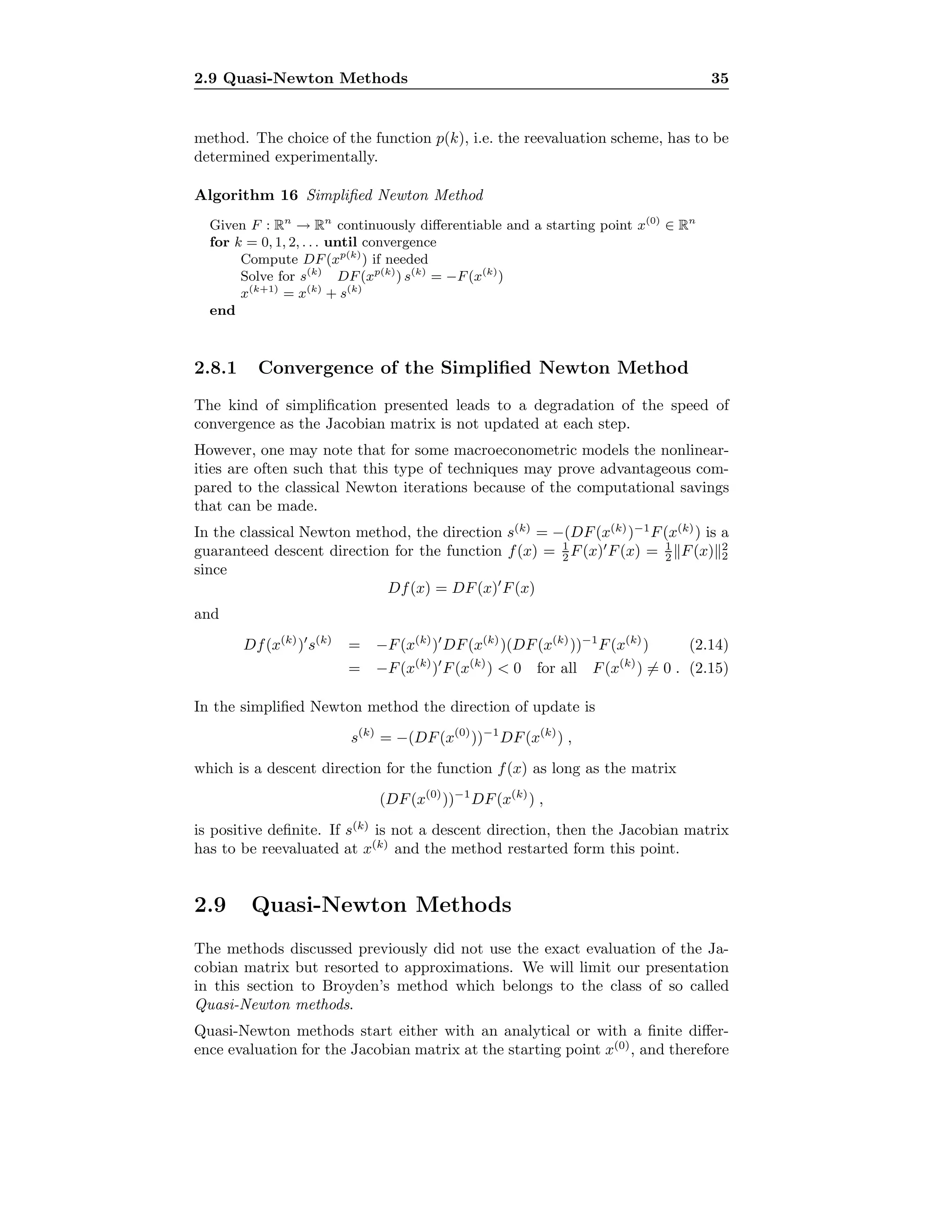
2.8 Simplified Newton Method
To avoid the repeated evaluation of the Jacobian matrix DF(x(k)
) at each step k,
one may reuse the first evaluation DF(x(0)
) for all subsequent steps k = 1, 2, . . . .
This method is called simplified Newton method and it is attractive when the
level of nonlinearity of F is not too high, since then the Jacobian matrix does
not vary too much.
Another advantage of this simplification is that the linear system to be solved at
each step is the same for different right-hand sides, leading to significant savings
in the computational work.
As discussed before, the computationally expensive steps in the Newton method
are the evaluation of the Jacobian matrix and the solution of the corresponding
linear system. If a direct method is applied in the simplified method, these two
steps are carried out only once and, for subsequent iterations, only the forward
and back substitution phases are needed.
In the one dimensional case, this technique corresponds to a parallel-chord
method. The first chord is taken to be the tangent to the point at coordi-
nates (x(0)
, F(x(0)
)) and for the next iterations this chord is simply shifted in a
parallel way.
To improve the convergence of this method, DF may occasionally be reevaluated
by choosing an integer increasing function p(k) with values in the interval [0, k]
and the linear system DF(x(p(k))
)s(k)
= −F(x(k)
) solved.
In the extreme case where p(k) = 0 , ∀k we have the simplified Newton method
and, at the other end, when p(k) = k , ∀k we have the classical Newton](https://image.slidesharecdn.com/c12cdca8-ad4d-451a-b4fb-6c6bd72ac4d1-161015164104/75/t-42-2048.jpg)
![2.9 Quasi-Newton Methods 36
compute x(1)
like the classical Newton method does. For the successive steps,
DF(x(0)
)—or an approximation J(0)
to it—is updated using (x(0)
, F(x(0)
)) and
(x(1)
, F(x(1)
)). The matrix DF(x(1)
) then can be approximated at little addi-
tional cost by a secant method.
The secant approximation A(1)
satisfies the equation
A(1)
(x(1)
− x(0)
) = F(x(1)
) − F(x(0)
) . (2.16)
Matrix A(1)
is obviously not uniquely defined by relation (2.16).
Broyden [20] introduced a criterion which leads to choosing—at the generic step
k—a matrix A(k+1)
defined as
A(k+1)
= A(k)
+
(y(k)
− A(k)
s(k)
) s(k)
s(k) s(k)
(2.17)
where y(k)
= F(x(k+1)
) − F(x(k)
)
and s(k)
= x(k+1)
− x(k)
.
Broyden’s method updates matrix A(k)
by a rank one matrix computed only
from the information of the current step and the preceding step.
Algorithm 17 Quasi-Newton Method using Broyden’s Update
Given F : Rn
→ Rn
continuously differentiable and a starting point x(0)
∈ Rn
Evaluate A(0)
by DF(x(0)
) or J(0)
for k = 0, 1, 2, . . . until convergence
Solve for s(k)
A(k)
s(k)
= −F(x(k)
)
x(k+1)
= x(k)
+ s(k)
y(k)
= F(x(k+1)
) − F(x(k)
)
A(k+1)
= A(k)
+ ((y(k)
− A(k)
s(k)
) s(k)
)/(s(k)
s(k)
)
end
Broyden’s method may generate sequences of matrices {A(k)
}k=0,1,... which do
not converge to the Jacobian matrix DF(x∗
), even though the method produces
a sequence {x(k)
}k=0,1,... converging to x∗
.
Dennis and Mor´e [25] have shown that the convergence behavior of the method
is superlinear under the same conditions as for Newton-type techniques. The
underlying reason that enables this favorable behavior is that A(k)
−DF(x(k)
)
stays sufficiently small.
From a computational standpoint, Broyden’s method is particularly attractive
since the solution of the successive linear systems A(k)
s(k)
= −F((k)
) can be
determined by updating the initial factorization of A(0)
for k = 1, 2, . . . . Such
an update necessitates O(n2
) operations, therefore reducing the original O(n3
)
cost of a complete refactorization.
Practically, the QR factorization update is easier to implement than the LU
update, see Gill et al. [47, pp. 125–150]. For sparse systems, however, the
advantage of the updating process vanishes.
A software reference for Broyden’s method is MINPACK by Mor´e, Garbow and
Hillstrom available on NETLIB.](https://image.slidesharecdn.com/c12cdca8-ad4d-451a-b4fb-6c6bd72ac4d1-161015164104/75/t-44-2048.jpg)
![2.10 Nonlinear First-order Methods 37
2.10 Nonlinear First-order Methods
The iterative techniques for the solution of linear systems described in sec-
tions 2.4.1 to 2.4.4 can be extended to nonlinear equations.
If we interpret the stationary iterations in algorithms 1 to 4 in terms of obtaining
x
(k+1)
i as the solution of the j-th equation with the other (n − 1) variables held
fixed, we may immediately apply the same idea to the nonlinear case.
The first issue is then the existence of a one-to-one mapping between the set
of equations {fi , i = 1, . . . , n} and the set of variables {xi , i = 1, . . . , n}.
This mapping is also called a matching and it can be shown that its existence
is a necessary condition for the solution to exist, see Gilli [50] or Gilli and
Garbely [51].
A matching m must be provided in order to define the variable m(i) that has
to be solved from equation i. For the method to make sense, the solution of
the i-th equation with respect to xm(i) must exist and be unique. This solution
can then be computed using a one dimensional solution algorithm—e.g. a one
dimensional Newton method.
We can then formulate the nonlinear Jacobi algorithm.
Algorithm 18 Nonlinear Jacobi Method
Given a matching m and a starting point x(0)
∈ Rn
Set up the equations so that m(i) = i for i = 1, . . . , n
for k = 0, 1, 2, . . . until convergence
for i = 1, . . . , n
Solve for xi
fi(x
(k)
1 , . . . , xi, . . . , x
(k)
n ) = 0
and set x
(k+1)
i = xi
end
end
The nonlinear Gauss-Seidel is obtained by modifying the “solve” statement.
Algorithm 19 Nonlinear Gauss-Seidel Method
Given a matching m and a starting point x(0)
∈ Rn
Set up the equations so that m(i) = i for i = 1, . . . , n
for k = 0, 1, 2, . . . until convergence
for i = 1, . . . , n
Solve for xi
fi(x
(k+1)
1 , . . . , x
(k+1)
i−1 , xi, x
(k)
i+1, . . . , x
(k)
n ) = 0
and set x
(k+1)
i = xi
end
end
In order to keep notation simple, we will assume from now on that the equations
and variables have been set up so that we have m(i) = i for i = 1, . . . , n.
The nonlinear SOR and FGS6
algorithms are obtained by a straightforward
6As already mentioned in the linear case, the FGS method should be considered as a second](https://image.slidesharecdn.com/c12cdca8-ad4d-451a-b4fb-6c6bd72ac4d1-161015164104/75/t-45-2048.jpg)
![2.10 Nonlinear First-order Methods 38
modification of the corresponding linear versions.
If it is possible to isolate xi from fi(x1, . . . , xn) for all i, then we have a normal-
ized system of equations. This is often the case in systems of equations arising
in macroeconometric modeling. In such a situation, each variable is isolated as
follows,
xi = gi(x1, . . . , xi−1, xi+1, . . . , xn), i = 1, 2, . . ., n . (2.18)
The “solve” statement in Algorithm 18 and Algorithm 19 is now dropped since
the solution is given in an explicit form.
2.10.1 Convergence
The matrix form of these nonlinear iterations can be found by linearizing the
equations around x(k)
, which yields
A(k)
x(k)
= b(k)
,
where A(k)
= DF(x(k)
) and b(k)
denotes the constant part of the linearization
of F. As the path of the iterates {x(k)
}k=0,1,2,... yields to different matrices
A(k)
and vectors b(k)
, the nonlinear versions of the iterative methods can no
longer be considered stationary methods. Each system A(k)
x(k)
= b(k)
will have
a different convergence behavior not only according to the splitting of A(k)
and
the updating technique chosen, but also because the values of the elements in
matrix A(k)
and vector b(k)
change from an iteration to another.
It follows that convergence criteria can only be stated for starting points x(0)
within a neighborhood of the solution x∗
. Similarly to what has been presented
in Section 2.4.6, we can evaluate the matrix B that governs the convergence
at x∗
and state that, if ρ(B) < 1, then the method is likely to converge. The
difficulty is that now the eigenvalues, and hence the spectral radius, vary with
the solution path. The same is also true for the optimal values of the parameters
ω and γ of the SOR and FGS methods.
In such a framework, Hughes Hallett [69] suggests several ways of computing
approximate optimal values for γ during the iterations. The simplest form is to
take
γk = (1 ± |x
(k)
i /x
(k−2)
i |)−1
,
the sign being positive if the iterations are cycling and negative if the itera-
tions are monotonic; xi is the element which violates the most the convergence
criterion.
One should also constrain γk to lie in the interval [0, 2], which is a necessary
condition for the FGS to converge. To avoid large fluctuations of γk, one may
smooth the sequence by the formula
˜γk = αkγk + (1 − αk)γk−1 ,
where αk is chosen in the interval [0, 1]. We may note that such strategies can
also be applied in the linear case to automatically set the value for γ.
order method.](https://image.slidesharecdn.com/c12cdca8-ad4d-451a-b4fb-6c6bd72ac4d1-161015164104/75/t-46-2048.jpg)
![2.11 Solution by Minimization 39
2.11 Solution by Minimization
In the preceding sections, methods for the solution of nonlinear systems of equa-
tions have been considered. An alternative to compute a solution of F(x) = 0
is to minimize the following objective function
f(x) = F(x) a , (2.19)
where · a denotes a norm in Rn
.
A reason that motivates such an alternative is that it introduces a criterion
to decide whether x(k+1)
is a better approximation to x∗
than x(k)
. As at the
solution F(x∗
) = 0, we would like to compare the vectors F(x(k+1)
) and F(x(k)
),
and to do so we compare their respective norms. What is required7
is that
F(x(k+1)
) a < F(x(k)
) a ,
which then leads us to the minimization of the objective function (2.19).
A convenient choice is the standard euclidian norm, since it permits an analytical
development of the problem. The minimization problem then reads
min
x
f(x) =
1
2
F(x) F(x) , (2.20)
where the factor 1/2 is added for algebraic convenience.
Thus methods for nonlinear least-squares problem, such as Gauss-Newton or
Levenberg-Marquardt, can immediately be applied to this framework. Since
the system is square and has a solution, we expect to have a zero residual
function f at x∗
.
In general it is advisable to take advantage of the structure of F to directly
approach the solution of F(x) = 0. However, in some circumstances, resorting to
the minimization of f(x) constitutes an interesting alternative. This is the case
when the nonlinear equations contain numerical inaccuracies preventing F(x) =
0 from having a solution. If the residual f(x) is small, then the minimization
approach is certainly preferable.
To devise a minimization algorithm for f(x), we need the gradient Df(x) and
the Hessian matrix D2
f(x), that is
Df(x) = DF(x) F(x) (2.21)
D2
f(x) = DF(x) DF(x) + Q(x) (2.22)
with Q(x) =
n
i=1
fi(x)D2
fi(x) .
We recall that F(x) = [f1(x) . . . fn(x)] , each fi(x) is a function from Rn
into R
and that each D2
fi(x) is therefore the n × n Hessian matrix of fi(x).
The Gauss-Newton method approaches the solution by computing a Newton
step for the first order conditions of (2.20), Df(x) = 0. At step k the Newton
7The iterate x(k+1) computed for instance by a classical Newton step does not necessarily
satisfy this requirement.](https://image.slidesharecdn.com/c12cdca8-ad4d-451a-b4fb-6c6bd72ac4d1-161015164104/75/t-47-2048.jpg)

![2.12 Globally Convergent Methods 41
0 2 4 6
-2
0
2
4
6
8
10
F(x)
0 2 4 6
0
10
20
30
40
f(x) = F(x)'*F(x)/2
Figure 2.1: A one dimensional function F(x) with a unique zero and its corre-
sponding function f(x) with multiple local minima.
2.12 Globally Convergent Methods
We saw in Section 2.6 that the Newton method is quadratically convergent when
the starting guess x(0)
is close enough to x∗
. An issue with the Newton method
is that when x(0)
is not in a convergent neighborhood of x∗
, the method may
not converge at all.
There are different strategies to overcome this difficulty. All of them first con-
sider the Newton step and modify it only if it proves unsatisfactory. This ensures
that the quadratic behavior of the Newton method is maintained near the so-
lution.
Some of the methods proposed resort to a hybrid strategy, i.e. they allow to
switch their search technique to a more robust method when the iterate is not
close enough to the solution.
It is possible to devise a hybrid method by combining a Newton-like method
and a quasirandom search (see e.g. Hickernell and Fang [65]), whereas an al-
ternative is to expand the radius of convergence and try to diminish the com-
putational cost by switching between a Gauss-Seidel and a Newton-like method
as in Hughes Hallett et al. [71]. Other such hybrid methods can be imagined
by turning to a more robust—though less rapid—technique when the Newton
method does not provide a satisfactory step.
The second modification amounts to building a model-trust region and we take
some combination of the Newton direction for F(x) = 0 and the steepest descent
direction for minimizing f(x).
2.12.1 Line-search
As already mentioned, a criterion to decide whether a Newton step is acceptable
is to impose a decrease in f(x). We also know that
s(k)
= (DF(x(k)
))−1
F(x(k)
)](https://image.slidesharecdn.com/c12cdca8-ad4d-451a-b4fb-6c6bd72ac4d1-161015164104/75/t-49-2048.jpg)
![2.12 Globally Convergent Methods 42
is a descent direction for f(x) since Df(x(k)
) s(k)
< 0, see Equation 2.14 on
page 35.
The idea is now to adjust the length of s(k)
by a factor ωk to provide a step
ωks(k)
that leads to a decrease in f. The simple condition f(x(k+1)
) < f(x(k)
)
is not sufficient to ensure that the sequence of iterates {x(k)
}k=0,1,2,... will lead
to x∗
. The issue is that either the decreases of f could be too small compared to
the length of the steps or that the steps are too small compared to the decrease
of f.
The problem can be fixed by imposing bounds on the decreases of ω. We recall
that ω = 1 first has to be tried to retain the quadratic convergence of the
method. The value of ω is chosen in a way such as it minimizes a model built
on the information available. Let us define
g(ω) = f(x(k)
+ ωs(k)
) ,
where s(k)
is the usual Newton step for solving F(x) = 0. We know the values
of
g(0) = f(x(k)
) = (1/2)F(x(k)
) F(x(k)
)
and
Dg(0) = Df(x(k)
) s(k)
= F(x(k)
) DF(x(k)
)s(k)
.
Since a Newton step is tried first we also have the value of g(1) = f(x(k)
+s(k)
).
If the inequality
g(1) > g(0) + αDg(0) , α ∈ (0, 0.5) (2.25)
is satisfied, then the decrease in f is too small and a backtrack along s(k)
is
introduced by diminishing ω. A quadratic model of g is built—using the infor-
mation g(0), g(1) and Dg(0)—to find the best approximate ω. The parabola is
defined by
ˆg(ω) = (g(1) − g(0) − Dg(0))w2
+ Dg(0)w + g(0) ,
and is illustrated in Figure 2.2.
The minimum value taken by g(ω), denoted ˆω, is determined by
Dˆg(ˆω) = 0 =⇒ ˆω =
−Dg(0)
2(g(1) − g(0) − Dg(0))
.
Lower and upper bounds for ˆω are usually set to constrain ˆω ∈ [0.1, 0.5] so that
very small or too large step values are avoided.
If ˆx(k)
= x(k)
+ ˆωs(k)
still does not satisfy (2.25), a further backtrack is per-
formed. As we now have a new item of information about g, i.e. g(ˆω), a cubic
fit is carried out.
The line-search can therefore be formalized as follows.](https://image.slidesharecdn.com/c12cdca8-ad4d-451a-b4fb-6c6bd72ac4d1-161015164104/75/t-50-2048.jpg)
![2.12 Globally Convergent Methods 43
-0.2 0 0.2 0.4 0.6 0.8 1
0
0.5
1
1.5
2
w
g(w)
Figure 2.2: The quadratic model ˆg(ω) built to determine the minimum ˆω.
Algorithm 20 Line-search with backtrack
Choose 0 < α < 0.5 (α = 10−4
)
and 0 < l < u < 1 (l = 0.1, u = 0.5)
wk = 1
while f(x(k)
+ wks(k)
) > f(x(k)
) + αωkDf(x(k)
) s(k)
Compute ˆwk by cubic interpolation
(or quadratic interpolation the first time)
end x(k+1)
= x(k)
+ ˆωks(k)
A detailed version of this algorithm is given in Dennis and Schnabel [26, Algo-
rithm A6.3.1].
2.12.2 Model-trust Region
The second alternative to modify the Newton step is to change not only its
length but also its direction.
The Newton step comes from a local model of the nonlinear function f around
x(k)
. The model-trust region explicitly limits the step length to a region where
this local model is reliable. We therefore impose to s(k)
to lie in such a region
by solving
s(k)
= argmins
1
2
DF(x(k)
)s + F(x(k)
) 2
2 (2.26)
subject to s 2 ≤ δk
for some δk > 0. The objective function (2.26) may also be written
1
2
s DF(x(k)
) DF(x(k)
)s + F(x(k)
) DF(x(k)
)s +
1
2
F(x(k)
) F(x(k)
) (2.27)
and problems arise when the matrix DF(x(k)
) DF(x(k)
) is not safely positive
definite, since the Newton step that minimizes (2.27) is
s(k)
= −(DF(x(k)
) DF(x(k)
))−1
DF(x(k)
) F(x(k)
) .](https://image.slidesharecdn.com/c12cdca8-ad4d-451a-b4fb-6c6bd72ac4d1-161015164104/75/t-51-2048.jpg)
![2.13 Stopping Criteria and Scaling 44
We can detect that this matrix becomes close to singularity for instance by
checking when κ2 ≥ u−1/2
, where u is defined as the unit roundoff of the com-
puter, see Section A.1.
In such a circumstance we decide to perturb the matrix by adding a diagonal
matrix to it and get
DF(x(k)
)DF(x(k)
) + λkI where λk =
√
n u DF(x(k)
) DF(x(k)
) 1 . (2.28)
This choice of λk can be shown to satisfy
1
n
√
u
≤ κ2(DF(x(k)
) DF(x(k)
) + λkI) − 1 ≤ u−1/2
,
when DF(x(k)
) ≥ u1/2
.
Another theoretical motivation for a perturbation such as (2.28) is the following
result:
lim
λ→0+
(J J + λI)−1
J = J+
,
where J+
denotes the Moore-Penrose pseudoinverse. This can be shown using
the SVD decomposition.
2.13 Stopping Criteria and Scaling
In all the algorithms presented in the preceding sections, we did not spec-
ify a precise termination criterion. Almost all the methods would theoreti-
cally require an infinite number of iterations to reach the limit of the sequence
{x(k)
}k=0,1,2.... Moreover even the techniques that should converge in a finite
number of steps in exact arithmetic may need a stopping criterion in a finite
precision environment.
The decision to terminate the algorithm is of crucial importance since it deter-
mines which approximation to x∗
the chosen method will ultimately produce.
To devise a first stopping criterion, we recall that the solution x∗
of our problem
must satisfy F(x∗
) = 0. As an algorithm produces approximations to x∗
and
as we use a finite precision representation of numbers, we should test whether
F(x(k)
) is sufficiently close to the zero vector. A second way of deciding to stop
is to test that two consecutive approximations, for example x(k)
and x(k−1)
, are
close enough. This leads to considering two kinds of possible stopping criteria.
The first idea is to test F(x(k)
) < F for a given tolerance F > 0, but this test
will prove inappropriate. The differences in the scale of both F and x largely
influence such a test. If F = 10−5
and if any x yields an evaluation of F in the
range [10−8
, 10−6
], then the method may stop at an arbitrary point. However,
if F yields values in the interval [10−1
, 102
], the algorithm will never satisfy the
convergence criterion. The test F(x(k)
) ≤ F will also very probably take into
account the components of x differently when x is badly scaled, i.e. when the
elements in x vary widely.
The remedy to some of these problems is then to scale F and to use the infinity
norm. The scaling is done by dividing each component of F by a value di](https://image.slidesharecdn.com/c12cdca8-ad4d-451a-b4fb-6c6bd72ac4d1-161015164104/75/t-52-2048.jpg)
![2.13 Stopping Criteria and Scaling 45
selected so that fi(x)/di is of magnitude 1 for values of x not too close to x∗
.
Hence, the test SF F ∞ ≤ F where SF = diag(1/d1, . . . , 1/dn) should be safe.
The second criterion tests whether the sequence {x(k)
}k=0,1,2,... stabilizes itself
sufficiently to stop the algorithm. We might want to perform a test on the
relative change between two consecutive iterations such as
x(k)
− x(k−1)
x(k−1)
≤ x .
To avoid problems when the iterates converge to zero, it is recommended to use
the criterion
max
i
ri ≤ x with ri =
|x
(k)
i − x
(k−1)
i |
max{|x
(k)
i |, ¯xi}
,
where ¯xi > 0 is an estimate of the typical magnitude of xi. The number of
expected correct digits in the final value of x(k)
is approximately − log10( x).
In the case where a minimization approach is used, one can also devise a test on
the gradient of f, see e.g. Dennis and Schnabel [26, p. 160] and Gill et al. [46,
p. 306].
The problem of scaling in macroeconometric models is certainly an important
issue and it may be necessary to rescale the model to prevent computational
problems. The scale is usually chosen so that all the scaled variables have magni-
tude 1. We may therefore replace x by ˜x = Sxx where Sx = diag(1/¯x1, . . . , 1/¯xn)
is a positive diagonal matrix.
To analyze the impact of this change of variables, let us define ˜F(˜x) = F(S−1
x ˜x)
so that we get
D ˜F(˜x) = (S−1
x ) DF(S−1
x ˜x)
= S−1
x DF(x) ,
and the classical Newton step becomes
˜s = −(D ˜F(˜x))−1 ˜F(˜x)
= −(S−1
x DF(x))−1
F(x) .
This therefore results in scaling the rows of the Jacobian matrix. We typically
expect that such a modification will allow a better numerical behavior by avoid-
ing some of the issues due to large differences of magnitude in the numbers we
manipulate.
We also know that an appropriate row scaling will improve the condition number
of the Jacobian matrix. This is linked to the problem of finding a preconditioner,
since we could replace matrix Sx in the previous development by a general
nonsingular matrix approximating the inverse of (DF(x)) .](https://image.slidesharecdn.com/c12cdca8-ad4d-451a-b4fb-6c6bd72ac4d1-161015164104/75/t-53-2048.jpg)

![3.1 Blocktriangular Decomposition of the Jacobian Matrix 47
3.1 Blocktriangular Decomposition of the Jaco-
bian Matrix
The logical structure of a system of equations is already defined if we know
which variable appears in which equation. Hence, the logical structure is not
connected to a particular quantification of the model. Its analysis will provide
important insights into the functioning of a model, revealing robust properties
which are invariant with respect to different quantifications.
The first task consists in seeking whether the system of equations can be solved
by decomposing the original system of equations into a sequence of interde-
pendent subsystems. In other words, we are looking for a permutation of the
model’s Jacobian matrix in order to get a blocktriangular form. This step is par-
ticularly important as macroeconometric models almost always allow for such a
decomposition.
Many authors have analyzed such sparse structures: some of them, e.g. Duff et
al. [30], approach the problem using incidence matrices and permutations, while
others, for instance Gilbert et al. [44], Pothen and Fahn [88] and Gilli [50], use
graph theory. This presentation follows the lines of the latter papers, since we
believe that the structural properties often rely on concepts better handled and
analyzed with graph theory. A clear discussion about the uses of graph theory
in macromodeling can be found in Gilli [49] and Gilli [50].
We first formalize the logical structure as a graph and then use a methodology
based on graphs to analyse its properties. Graphs are used to formalize relations
existing between elements of a set. The standard notation for a graph G is
G = (X, A) ,
where X denotes the set of vertices and A is the set of arcs of the graph. An arc
is a couple of vertices (xi, xj) defining an existing relation between the vertex
xi and the vertex xj.
What is needed to define the logical structure of a model is its deterministic
part formally represented by the set of n equations
F(y, z) = 0 .
In order to keep the presentation simpler, we will assume that the model has
been normalized, i.e. a different left-hand side variable has been assigned to each
equation, so that we can write
yi = gi(y1, . . . , yi−1, yi+1, . . . , yn, z), i = 1, . . . , n .
We then see that there is a link going from the variables in the right-hand
side to the variable on the left-hand side. Such a link can be very naturally
represented by a graph G = (Y, U) where the vertices represent the variables yi,
i = 1, . . . , n and an arc (yj, yi) represents the link. The graph of the complete
model is obtained by putting together the partial graphs corresponding to all
single equations.
We now need to define the adjacency matrix AG = (aij) of our graph G = (Y, U).
We have
aij =
1 if and only if the arc (yj, yi) exists,
0 otherwise.](https://image.slidesharecdn.com/c12cdca8-ad4d-451a-b4fb-6c6bd72ac4d1-161015164104/75/t-55-2048.jpg)
![3.2 Orderings of the Jacobian Matrix 48
We may easily verify that the adjacency matrix AG has the same nonzero pattern
as the Jacobian matrix of our model. Thus, the adjacency matrix contains all
the information about the existing links between the variables in all equations
defining the logical structure of the model.
We already noticed that an arc in the graph corresponds to a link in the model.
A sequence of arcs from a vertex yi to a vertex yj is a path, which corresponds
to an indirect link in the model, i.e. there is a variable yi which has an effect
on a variable yj through the interaction of a set of equations.
A first task now consists in finding the sets of simultaneous equations of the
model, which correspond to irreducible diagonal matrices in the blockrecursive
decomposition; in the graph, this corresponds to the strong components. A
strong component is the largest possible set of interdependent vertices, i.e. the
set where any ordered pair for vertices (yi, yj) verifies a path from yi to yj and
a path from yj to yi. The strong components define a unique partition among
the equations of the model into sets of simultaneous equations. The algorithms
that find the strong components of a graph are standard and can be found
in textbooks about algorithmic graph theory or computer algorithms, see e.g.
Sedgewick [93, p. 482] or Aho et al. [2, p. 193].
Once the strong components are identified, we need to know in what order
they appear in the blocktriangular Jacobian matrix. A technique consists in
resorting to the reduced graph the vertices of which are the strong components
of the original graph and where there will be an arc between the new vertices,
if there is at least one arc between the vertices corresponding to the two strong
components considered. The reduced graph is without circuits, i.e. there are no
interdependencies and therefore it will be possible to number the vertices in a
way that there does not exist arcs going from higher numbered vertices to lower
numbered vertices. This ordering of the corresponding strong components in
the Jacobian matrix then exhibits a blocktriangular pattern. We may mention
that Tarjan’s algorithm already identifies the strong components in the order
described above.
The solution of the complete model can now be performed by considering the
sequence of submodels corresponding to the strong components. The effort put
into the finding the blocktriangular form is negligible compared to the complex-
ity of the model-solving. Moreover, the increased knowledge of which parts of
the model are dependent or independent of others is very helpful in simulation
exercises.
The usual patterns of the blocktriangular Jacobian matrix corresponding to
macroeconometric models exhibits a single large interdependent block, which is
both preceeded and followed by recursive equations. This pattern is illustrated
in Figure 3.1.
3.2 Orderings of the Jacobian Matrix
Having found the blocktriangular decomposition, we now switch our attention
to the analysis of the structure of an indecomposable submodel. Therefore,
the Jacobian matrices considered in the following are indecomposable and the](https://image.slidesharecdn.com/c12cdca8-ad4d-451a-b4fb-6c6bd72ac4d1-161015164104/75/t-56-2048.jpg)
![3.2 Orderings of the Jacobian Matrix 49
..............................................
...................
.....................................
0
.
.
.
.
.
.
.
.
.
.
.
.
.
.
.
.
.
.
.
.
.
.
.
.
.
.
.
.
.
.
.
.
.
.
.
.
.
.
.
.
.
.
.
.
.
.
.
.
.
.
.
.
.
.
.
.
.
.
.
.
.
.
.
.
.
.
.
.
.
.
.
.
.
.
.
.
.
.
.
.
.
.
.
.
.
.
.
.
.
.
.
.
.
.
.
.
.
.
.
.
.
.
.
.
.
.
.
.
.
.
.
.
.
.
.
.
.
.
.
.
.
.
.
.
.
.
.
.
.
.
.
.
.
.
.
.
.
.
.
.
.
.
.
.
.
.
.
.
.
.
.
.
.
.
.
.
.
.
.
.
.
.
.
.
.
.
.
.
.
.
.
.
.
.
.
.
.
.
.
.
.
.
.
.
.
.
.
.
.
.
.
.
.
.
.
.
.
.
.
.
.
.
.
.
.
.
.
.
.
.
.
.
.
.
.
.
.
.
.
.
.
.
.
.
.
.
.
.
.
.
.
.
.
.
.
.
.
.
.
.
.
.
.
.
.
.
.
.
.
.
.
.
.
...
......................
......................
......................
......................
......................
......................
......................
......................
......................
......................
......................
......................
......................
......................
......................
......................
......................
......................
......................
......................
......................
......................
......................
......................
......................
......................
......................
......................
......................
......................
......................
......................
......................
......................
......................
......................
......................
......................
......................
......................
......................
......................
......................
......................
......
.....
......
.....
......
.....
......
.....
......
.....
......
Figure 3.1: Blockrecursive pattern of a Jacobian matrix.
corresponding graph is a strong component.
Let us consider a directed graph G = (V, A) with n vertices and the correspond-
ing set C = {c1, . . . , cp} of all elementary circuits of G. An essential set S of
vertices is a subset of V which covers the set C, where each circuit is consid-
ered as the union set of vertices it contains. According to Guardabassi [57], a
minimal essential set is an essential set of minimum cardinality, and it can be
seen as a problem of minimum cover, or as a problem of minimum transversal
of a hypergraph with edges defined by the set C.
For our Jacobian matrix, the essential set will enable us to find orderings such
that the sets S and F in the matrices shown in Figure 3.2 are minimal. The set
S corresponds to a subset of variables and the set F to a subset of feedbacks
(entries above the diagonal of the Jacobian matrix). The set S is also called the
essential feedback vertex set and the set F is called the essential feedback arc
set.
..............................................................................................................................................................................................................................
......................................................................................................................................................................................................................
.........................................................
0
.
.
.
.
.
.
.
.
.
.
.
.
.
.
.
.
.
.
.
.
.
.
.
.
.
.
.
.
.
.
.
.
.
.
.
.
.
.
.
.
.
.
.
.
.
.
.
.
.
.
.
.
.
.
.
.
.
.
.
.
.
.
.
.
.
.
.
.
.
.
.
.
.
.
.
.
.
.
.
.
.
.
.
.
.
.
.
.
.
.
.
.
.
.
.
.
.
.
.
.
.
.
.
.
.
.
.
.
.
.
.
.
.
.
.
.
.
.
.
.
.
.
.
.
.
.
.
.
.
.
.
.
.
.
.
.
.
.
.
.
.
.
.
.
.
.
.
.
.
.
.
.
.
.
.
.
.
.
.
.
.
.
.
.
.
.
.
.
.
.
.
.
.
.
.
.
.
.
.
.
.
.
.
.
.
.
.
.
.
.
.
.
.
.
.
.
.
.
.
.
.
.
.
.
.
.
.
.
.
.
.
.
.
.
.
.
.
.
.
.
.
.
.
.
.
.
.
.
.
.
.
.
.
.
.
.
.
.
.
.
.
.
.
.
.
.
.
.
.
.
.
.
.
.
.
.
.
.
.
.
.
.
.
.
.
.
.
.
.
.
.
.
.
.
.
.
.
.
.
.
.
.
.
.
.
.
.
.
.
.
.
.
.
.
.
.
.
.
.
.
.
.
.
.
.
.
.
.
.
.
.
.
.
.
.
.
.
.
.
.
.
.
.
.
.
.
.
.
.
.
.
.
.
.
.
.
.
.
.
.
.
.
.
.
.
.
.
.
.
.
.
.
.
.
.
.
.
.
.
.
.
.
.
.
.
.
.
.
.
.
.
.
.
.
.
.
.
.
.
.
.
.
.
.
.
.
.
.
.
.
.
.
.
.
.
.
.
.
.
.
.
.
.
.
.
.
.
.
.
.
.
.
.
.
.
.
.
.
.
.
.
.
.
.
.
.
.
.
.
.
.
.
.
.
.
.
.
.
.
.
.
.
.
.
.
.
.
.
.
.
.
.
.
.
.
.
.
.
.
.
.
.
.
.
.
.
.
.
.
.
.
.
.
.
.
.
.
.
.
.
.
.
.
.
.
.
.
.
.
.
.
.
.
.
.
.
.
.
.
.
.
.
.
.
.
.
.
.
.
.
.
.
.
.
.
.
.
.
.
.
.
.
.
.
.
.
.
.
.
.
.
.
.
.
.
.
.
.
.
.
.
.
.
.
.
.
.
.
.
.
.
.
.
.
.
.
.
.
.
.
.
.
.
.
.
.
.
.
.
.
.
.
.
.
.
.
.
.
.
.
.
.
.
.
.
.
.
.
.
.
.
.
.
.
.
.
.
.
.
.
.
.
.
.
.
.
.
.
.
.
.
.
.
.
.
.
.
.
.
.
.
.
.
.
.
.
.
.
.
.
.
.
.
.
.
.
.
.
.
.
.
.
.
.
.
.
.
.
.
.
.
.
.
.
.
.
.
.
.
.
.
.
.
.
.
.
.
.
.
.
.
.
.
.
.
.
.
.
.
.
.
.
.
.
.
.
.
.
.
.
.
.
.
.
.
.
.
.
.
.
.
.
.
.
.
.
.
.
.
.
.
.
.
.
.
.
.
.
.
.
.
.
.
.
.
.
.
.
.
.
.
.
.
.
.
.
.
.
.
.
.
.
.
.
.
.
.
.
.
.
.
.
.
.
.
.
.
.
.
.
.
.
.
.
.
.
.
.
.
.
.
.
.
.
.
.
.
.
.
.
.
.
.
.
.
.
.
.
.
.
.
.
.
.
.
.
.
.
.
.
.
.
.
.
.
.
.
.
.
.
.
.
.
.
.
.
.
.
.
.
.
.
.
.
.
.
.
.
.
.
.
.
.
.
S
(a)
..............................................................................................................................................................................................................................................................................................................
×
×
×
×
F
.
.
.
.
.
.
.
.
.
.
.
.
.
.
.
.
.
.
.
.
.
.
.
.
.
.
.
.
.
.
.
.
.
.
.
.
.
.
.
.
.
.
.
.
.
.
.
.
.
.
.
.
.
.
.
.
.
.
.
.
.
.
.
.
.
.
.
.
.
.
.
.
.
.
.
.
.
.
.
.
.
.
.
.
.
.
.
.
.
.
.
.
.
.
.
.
.
.
.
.
.
.
.
.
.
.
.
.
.
.
.
.
.
.
.
.
.
.
.
.
.
.
.
.
.
.
.
.
.
.
.
.
.
.
.
.
.
.
.
.
.
.
.
.
.
.
.
.
.
.
.
.
.
.
.
.
.
.
.
.
.
.
.
.
.
.
.
.
.
.
.
.
.
.
.
.
.
.
.
.
.
.
.
.
.
.
.
.
.
.
.
.
.
.
.
.
.
.
.
.
.
.
.
.
.
.
.
.
.
.
.
.
.
.
.
.
.
.
.
.
.
.
.
.
.
.
.
.
.
.
.
.
.
.
.
.
.
.
.
.
.
.
.
.
.
.
.
.
.
.
.
.
.
.
.
.
.
.
.
.
.
.
.
.
.
.
.
.
.
.
.
.
.
.
.
.
.
.
.
.
.
.
.
.
.
.
.
.
.
.
.
.
.
.
.
.
.
.
.
.
.
.
.
.
.
.
.
.
.
.
.
.
.
.
.
.
.
.
.
.
.
.
.
.
.
.
.
.
.
.
.
.
.
.
.
.
.
.
.
.
.
.
.
.
.
.
.
.
.
.
.
.
.
.
.
.
.
.
.
.
.
.
.
.
.
.
.
.
.
.
.
.
.
.
.
.
.
.
.
.
.
.
.
.
.
.
.
.
.
.
.
.
.
.
.
.
.
.
.
.
.
.
.
.
.
.
.
.
.
.
.
.
.
.
.
.
.
.
.
.
.
.
.
.
.
.
.
.
.
.
.
.
.
.
.
.
.
.
.
.
.
.
.
.
.
.
.
.
.
.
.
.
.
.
.
.
.
.
.
.
.
.
.
.
.
.
.
.
.
.
.
.
.
.
.
.
.
.
.
.
.
.
.
.
.
.
.
.
.
.
.
.
.
.
.
.
.
.
.
.
.
.
.
.
.
.
.
.
.
.
.
.
.
.
.
.
.
.
.
.
.
.
.
.
.
.
.
.
.
.
.
.
.
.
.
.
.
.
.
.
.
.
.
.
.
.
.
.
.
.
.
.
.
.
.
.
.
.
.
.
.
.
.
.
.
.
.
.
.
.
.
.
.
.
.
.
.
.
.
.
.
.
.
.
.
.
.
.
.
.
.
.
.
.
.
.
.
...
(b)
Figure 3.2: Sparsity pattern of the reordered Jacobian matrix.
Such minimum covers are an important tool in the study of large scale inter-
dependent systems. A technique often used to understand and to solve such
complex systems consists in representing them as a directed graph which can
be made feedback-free by removing the vertices belonging to an essential set.1
1See, for instance, Garbely and Gilli [42] and Gilli and Rossier [54], where some aspects of
the algorithm presented here have been discussed.](https://image.slidesharecdn.com/c12cdca8-ad4d-451a-b4fb-6c6bd72ac4d1-161015164104/75/t-57-2048.jpg)
![3.2 Orderings of the Jacobian Matrix 50
However, in the theory of complexity, this problem of finding minimal essen-
tial sets—also referred to as the feedback-vertex-set problem—is known to be
NP-complete2
and we cannot hope to obtain a solution for all graphs.
Hence, the problem is not a new one in graph theory and system analysis,
where several heuristic and non-heuristic methods have been suggested in the
literature. See, for instance, Steward [94], Van der Giessen [98], Reid [89],
Bodin [16], Nepomiastchy et al. [83], Don and Gallo [27] for heuristic algorithms,
and Guardabassi [58], Cheung and Kuh [22] and Bhat and Kinariwala [14] for
nonheuristic methods.
The main feature of the algorithm presented here is to give all optimal solutions
for graphs corresponding in size and complexity to the commonly used large-
scale macroeconomic models in reasonable time.
The efficiency of the algorithm is obtained mainly by the generation of only a
subset of the set of all elementary circuits from which the minimal covers are
then computed iteratively by considering one circuit at a time. Section 3.2.1
describes the iterative procedure which uses Boolean properties of minimal
monomial, Section 3.2.1 introduces the appropriate transformations necessary
to reduce the size of the graph and Section 3.2.1 presents an algorithm for the
generation of the subset of circuits necessary to compute the covers.
Since any minimal essential set of G is given by the union of minimal essential
sets of its strong components, we will assume, without loss of generality, that G
has only one strong component.
3.2.1 The Logical Framework of the Algorithm
The particularity of the algorithm consists in the combination of three points:
a procedure which computes covers iteratively by considering one circuit at a
time, transformations likely to reduce the size of the graph, and an algorithm
which generates only a particular small subset of elementary circuits.
Iterative Construction of Covers
Let us first consider an elementary circuit ci of G as the following set of vertices
ci =
j∈Ci
{vj} , i = 1, . . . , p , (3.1)
where Ci is the index set for the vertices belonging to circuit ci. Such a circuit
ci can also be written as a sum of symbols representing the vertices, i.e.
j∈Ci
vj , i = 1, . . . , p . (3.2)
What we are looking for are covers, i.e. sets of vertices selected such as at least
one vertex is in each circuit ci, i = 1, . . . , p. Therefore, we introduce the product
2Proof for the NP-completeness are given in Karp [72], Aho et al. [2, pp. 378-384], Garey
and Johnson [43, p. 192] and Even [32, pp. 223-224].](https://image.slidesharecdn.com/c12cdca8-ad4d-451a-b4fb-6c6bd72ac4d1-161015164104/75/t-58-2048.jpg)
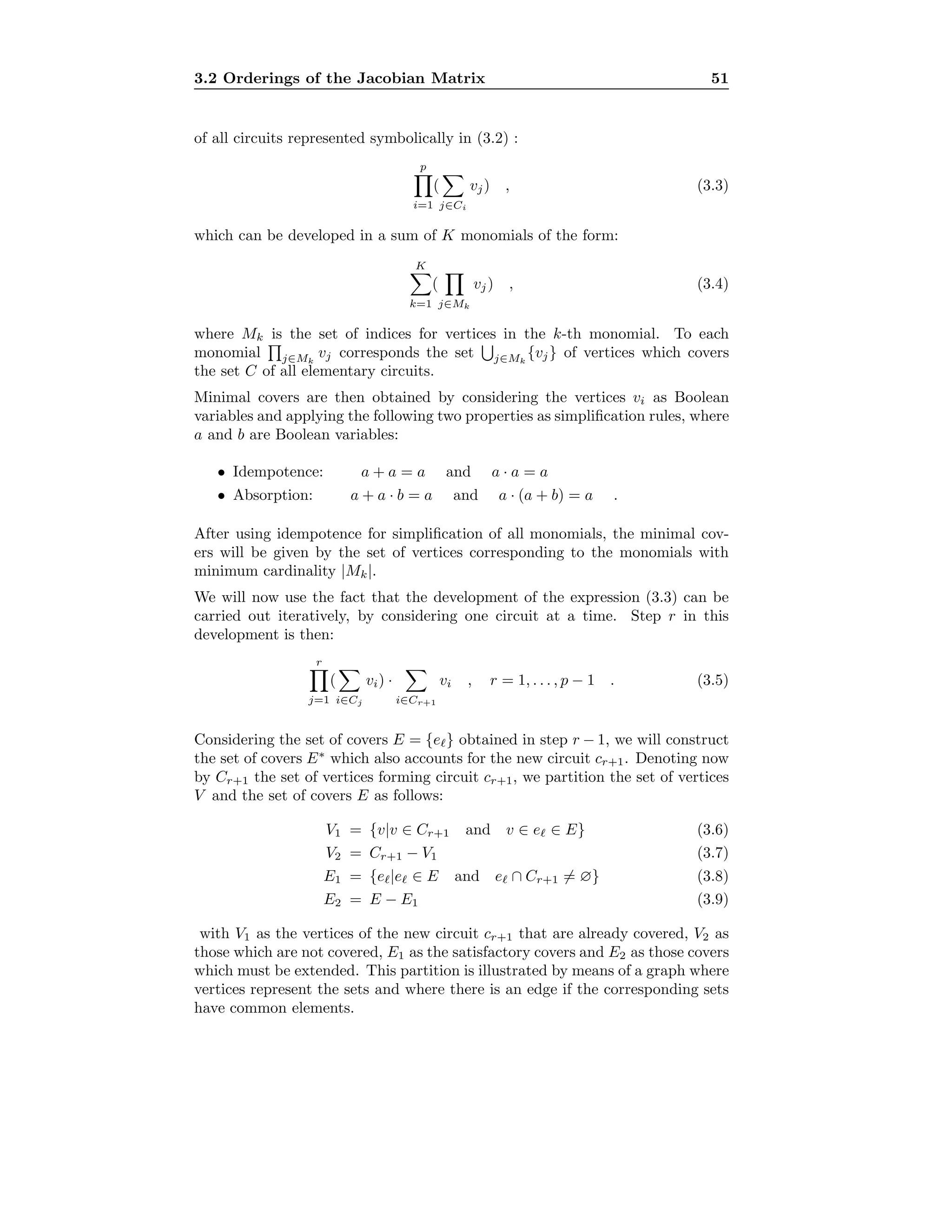
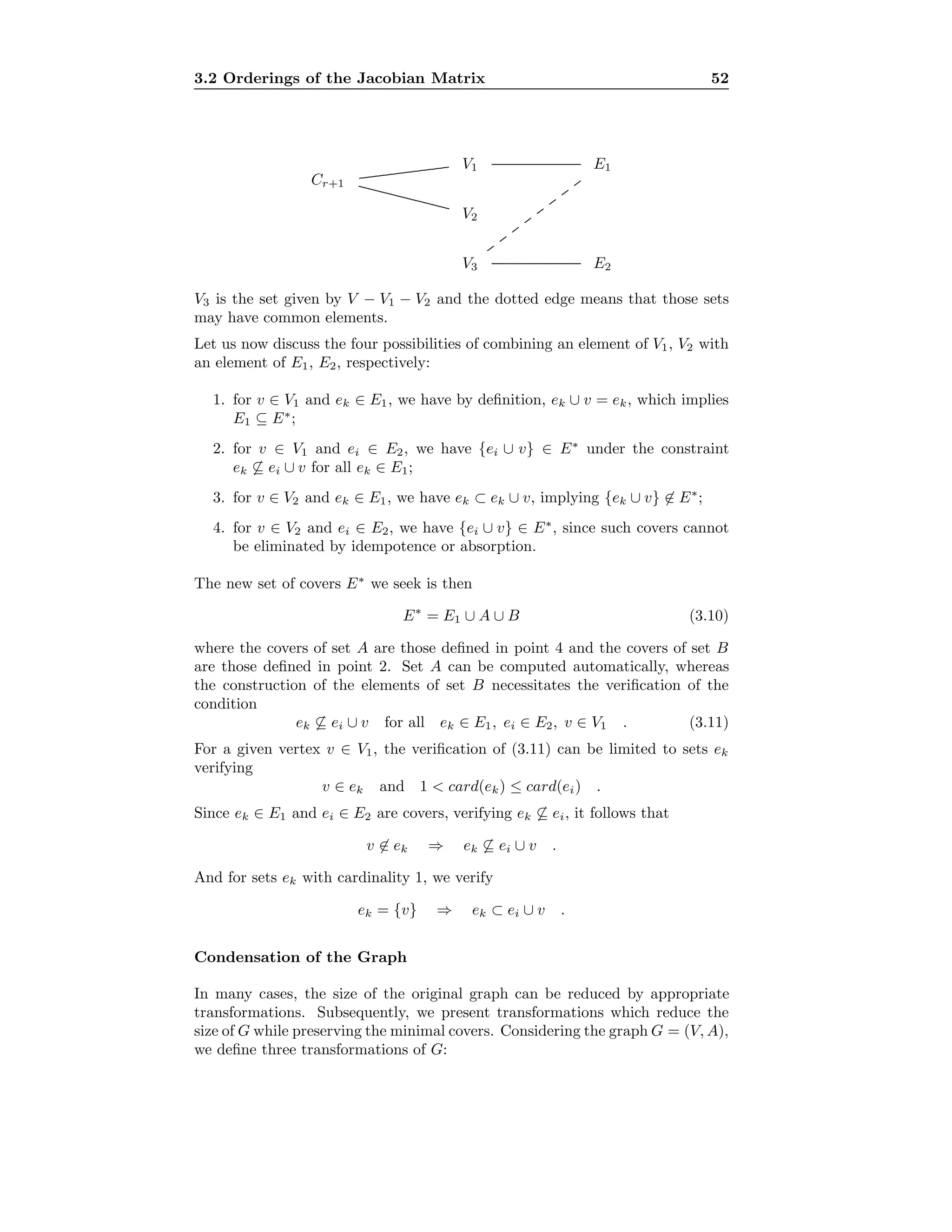

![3.2 Orderings of the Jacobian Matrix 54
Proof. By definition, any element of ei ∈ E will contain a vertex of circuit
cj. Therefore, as cj ⊂ cr+1, the set of partitions defined in (3.6–3.9) will verify
cj ⊂ V1 ⇒ E1 = E ⇒ E2 = ∅ and E∗
= E1 = E. 2
We will now discuss an efficient algorithm for the enumeration of only those
circuits which are not absorbed. This point is the most important, as we can
only expect efficiency if we avoid the generation of many circuits from the set
of all elementary circuits, which, of course, is of explosive cardinality.
In order to explore the circuits of the condensed graph systematically, we first
consider the circuits containing a given vertex v1, then consider the circuits
containing vertex v2 in the subgraph V − {v1}, and so on. This corresponds to
the following partition of the set of circuits C:
C =
n−1
i=1
Cvi , (3.12)
where Cvi denotes the set of all elementary circuits containing vertex vi in the
subgraph with vertex set V − {v1, . . . , vi−1}. It is obvious that Cvi ∩ Cvj = ∅
for i = j and that some sets Cvi will be empty.
Without loss of generality, let us start with the set of circuits Cv1 . The following
definition characterizes a subset of circuits of Cv1 which are not absorbed.
Definition 2 The circuit of length k + 1 defined by the sequence of vertices
[v1, x1, . . . , xk, v1] is a chordless circuit if G contains neither arcs of the form
(xi, xj) for j − i > 1, nor the arc (xi, v1) for i = k. Such arcs, if they exist, are
called chords.
In order to seek the chordless circuits containing the arc (v1, vk), let us consider
the directed tree T = (S, U) with root v1 and vertex set S = Adj(v1) ∪ Adj(vk).
The tree T enables the definition of a subset
AT = AV
T ∪ AS
T (3.13)
of arcs of the graph G = (V, A). The set
AV
T = {(xi, xj)|xi ∈ V − S and xj ∈ S} (3.14)
contains arcs going from vertices not in the tree to vertices in the tree. The set
AS
T = {(xi, xj)|xi, xj ∈ S and (xi, xj) ∈ U} (3.15)
contains the cross, back and forward arcs in the tree. The tree T is shown in
Figure 3.4, where the arcs belonging to AT are drawn in dotted lines. The set
Rvi denotes the adjacency set Adj(vi) restricted to vertices not yet in the tree.
Proposition 3 A chordless circuit containing the arc (v1, vk) cannot contain
arcs (vi, vj) ∈ AT .
Proof. The arc (v1, vk) constitutes a chord for all paths [v1, . . . , vk]. The arc
(vk, vi), vi ∈ Rvk
constitutes a chord for all paths [vk, . . . , vi]. 2](https://image.slidesharecdn.com/c12cdca8-ad4d-451a-b4fb-6c6bd72ac4d1-161015164104/75/t-62-2048.jpg)
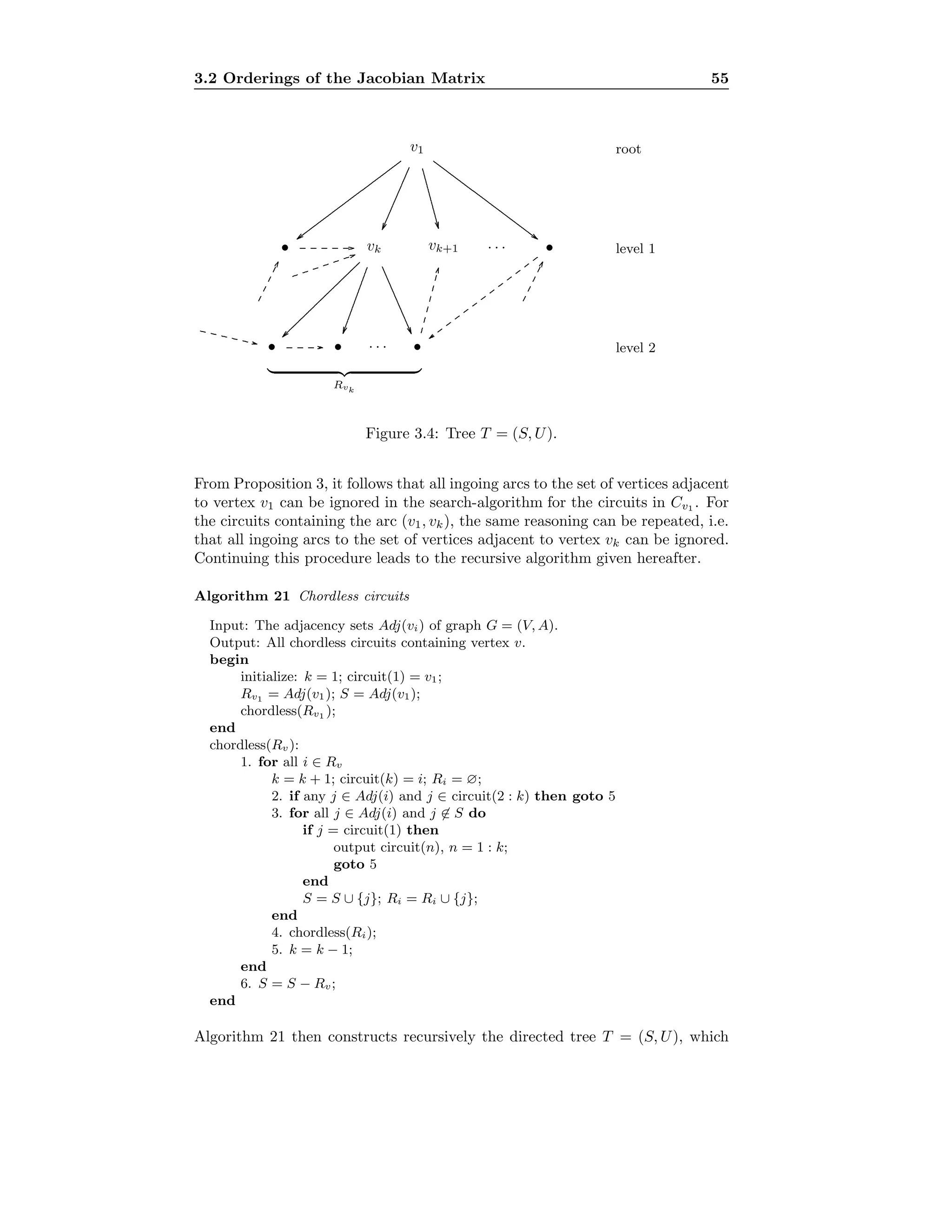
![3.3 Point Methods versus Block Methods 57
in Algorithm 2, is a point method.
We will show that, due to the particular structure of most macroeconomic mod-
els, the block method is not likely to constitute an optimal strategy. We also
discuss the convergence of first-order iterative techniques, with respect to order-
ings corresponding to different feedback arc sets, leaving, however, the question
of the optimal ordering open.
3.3.1 The Problem
We have seen in Section 2.10 that for a normalized system of equations the
generic iteration k for the point Gauss-Seidel method is written as
xk+1
i = gi(xk+1
1 , . . . , xk+1
i−1 , xk
i+1, . . . , xk
n) , i = 1, . . . , n . (3.16)
It is then obvious that (3.16) could be solved within a single iteration, if the
entries in the Jacobian matrix of the normalized equations, corresponding to the
xk
i+1, . . . , xk
n, for each equation i = 1, . . . , n, were zero.3
Therefore, it is often
argued that an optimal ordering for first-order iterative methods should yield
a quasi-triangular Jacobian matrix, i.e. where the nonzero entries in the upper
triangular part are minimum. Such a set of entries corresponds to a minimum
feedback arc set discussed earlier. For a given set F, the Jacobian matrix can
then be ordered as shown on panel (b) of Figure 3.2 already given before.
The complexity of Newton-like algorithms is O(n3
) which promises interesting
savings in computation if n can be reduced. Therefore, various authors, e.g.
Becker and Rustem [11], Don and Gallo [27] and Nepomiastchy and Ravelli [82],
suggest a reordering of the Jacobian matrix as shown on panel (a) of Figure 3.2.
The equations can therefore be partitioned into two sets
xR = gR(xR; xS) (3.17)
fS(xS; xR) = 0 , (3.18)
where xS are the variables defining the feedback vertex set S (spike variables).
Given an initial value for the variables xS, the solution for the variables xR is
obtained by solving the equations gR recursively. The variables xR are then
exogenous for the much smaller subsystem fS, which is solved by means of a
Newton-like method. These two steps of the block method in question are then
repeated until they achieve convergence.
3.3.2 Discussion of the Block Method
The advantages and inconveniences of first-order iterative methods and Newton-
like techniques have been extensively discussed in the literature. Recently, it has
been shown clearly by Hughes Hallett [70] that a comparison of the theoretical
performance between these two types of solution techniques is not possible.
As already mentioned, the solution of the original system, after the introduction
of the decomposition into the subsystems (3.17) and (3.18), is obtained by means
3Which then corresponds to a lower triangular matrix.](https://image.slidesharecdn.com/c12cdca8-ad4d-451a-b4fb-6c6bd72ac4d1-161015164104/75/t-65-2048.jpg)

![3.3 Point Methods versus Block Methods 59
3.3.3 Ordering and Convergence for First-order Iterations
The previous section clearly shows the interest of first-order iterative methods
for solving macroeconomic models. It is well-known that the ordering of the
equations is crucial for the convergence of first-order iterations. The ordering
we considered so far, is the result of a minimization of the cardinality nS of the
feedback vertex set S. However, such an ordering is, in general, not optimal.
Hereafter, we will introduce the notation used to study the convergence of first-
order iterative methods in relation with the ordering of the equations.
A linear approximation for the normalized system is given by
x = Ax + b , (3.24)
with A = ∂g
∂x , the Jacobian matrix evaluated at the solution x∗
and b repre-
senting exogenous and lagged variables. Splitting A into A = L + U with L and
U, respectively a lower and an upper triangular matrix, system (3.24) can then
be written as (I − L)x = Ux + b. Choosing Gauss-Seidel’s first-order iterations
(see Section 2.10), the k-th step in the solution process of our system is
(I − L)x(k+1)
= Ux(k)
+ b , k = 0, 1, 2, . . . (3.25)
where x(0)
is an initial guess for x. It is well known that the convergence of
(3.25) to the solution x∗
can be investigated on the error equation
(I − L)e(k+1)
= Ue(k)
,
with e(k)
= x∗
− x(k)
as the error for iteration k. Setting B = (I − L)−1
U and
relating the error e(k)
to the original error e(0)
we get
ek
= Bk
e0
, (3.26)
which shows that the necessary and sufficient condition for the error to converge
to zero is that Bk
converges to a zero matrix, as presented in Section 2.4.6. This
is guaranteed if all eigenvalues λi of matrix B verify |λi| < 1.
The convergence then clearly depends upon a particular ordering of the equa-
tions. If the Jacobian matrix A is a lower triangular matrix, then the algorithm
will converge within one iteration. This suggests choosing a permutation of A
so that U is as “small” as possible.
Usually, the “magnitude” of matrix U is defined in terms of the number of
nonzero elements. The essential feedback arc set, defined in Section 3.2, defines
such matrices U which are “small”. However, we will show that such a criterion
for the choice of matrix U is not necessarily optimal for convergence. In general,
there are several feedback arc sets with minimum cardinality and the question
of which one to choose arises.
Without a theoretical framework from which to decide about such a choice, we
resorted to an empirical investigation of a small macroeconomic model.4
The
size n of the Jacobian matrix for this model is 28 and there exist 76 minimal
feedback arc sets5
ranging from cardinality 9 to cardinality 15. We solved the
4The City University Business School (CUBS) model of the UK economy [13].
5These sets have been computed with the program Causor [48].](https://image.slidesharecdn.com/c12cdca8-ad4d-451a-b4fb-6c6bd72ac4d1-161015164104/75/t-67-2048.jpg)
![3.3 Point Methods versus Block Methods 60
CUBS model using all the orderings corresponding to these 76 essential feedback
arc sets. We observed that convergence has been achieved, for a given period, in
less than 20 iterations by 70% of the orderings. One ordering needs 250 iterations
to converge and surprisingly 8 orderings do not converge at all. Moreover, we
did not observe any relation between the cardinality of the essential feedback arc
set and the number of iterations necessary to converge to the solution. Among
others, we tried to weigh matrix U by means of the sum of the squared elements.
Once again, we came to the conclusion that there is no relationship between the
weight of U and the number of iterations.
Trying to characterize the matrix U which achieves the fastest convergence, we
chose to systematically explore all possible orderings for a four equations linear
system. We calculated λmax = maxi |λi| for each matrix B corresponding to the
orderings. We observed that the n! possible orderings produce at most (n − 1)!
distinct values for λmax. Again, we verified that neither the number of nonzero
elements in matrix U nor their value is related to the values for λmax.
i1 i2
i3 i4
................................................................................... ...........
...................................................................................
...........
.................................................................................................................................
...........
...................................................................................
...........
................................................................................... ...........
....................................................................................................................................................................................................................................................................................................................... ...........
.........................................................................................................................................................................................................................................................................................................................
a
.5
−.4
−1.3
2
.6
−.65
1 2 3 4
1 −1 0 0 −.65
2 .5 −1 0 0
3 −.4 −1.3 −1 0
4 .6 2 a −1
3 1 2 4
3 −1 −.4 −1.3 0
1 0 −1 0 −.65
2 0 .5 −1 0
4 a .6 2 −1
Figure 3.5: Numerical example showing the structure is not sufficient.
Figure 3.5 displays the graph representing the four linear equations and matrices
A − I corresponding to two particular orderings—[1, 2, 3, 4] and [3, 1, 2, 4]—of
these equations.
If the value of the coefficient a is .7, then the ordering [1, 2, 3, 4], corresponding
to matrix U with a single element, has the smallest possible λmax = .56. If we
take the equations in the order [3, 1, 2, 4], we get λmax = 1.38.
Setting the value of coefficient a at −.7 produces the opposite. The ordering
[3, 1, 2, 4] which does not minimize the number of nonzero elements in matrix U
gives λmax = .69, whereas the ordering [1, 2, 3, 4] gives λmax = 1.52.
This example clearly shows that the structure of the equations in itself is not a
sufficient information to decide on a good ordering of the equations.
Having analyzed the causal structure of many macroeconomic models, we ob-
served that the subset of equations corresponding to a feedback vertex set (spike
variables) happens to be almost always recursive. For models of this type, it is
certainly not indicated to use a Newton-type technique to solve the submodel
within the block method. Obviously, in such a case, the block method is equiv-
alent to a first-order iterative technique applied to the complete system. The
crucial question is then, whether a better ordering than the one derived from
the block method exists.](https://image.slidesharecdn.com/c12cdca8-ad4d-451a-b4fb-6c6bd72ac4d1-161015164104/75/t-68-2048.jpg)
![3.4 Essential Feedback Vertex Sets and the Newton Method 61
3.4 Essential Feedback Vertex Sets and the New-
ton Method
In general the convergence of Newton-type methods is not sensitive to different
orderings of the Jacobian matrix. However, from a computational point of view
it can be interesting to reorder the model so that the Jacobian matrix shows the
pattern displayed in Figure 3.2 panel (a). This pattern is obtained by computing
an essential feedback vertex set as explained in Section 3.2.
One way to exploit this ordering is to condense the system into one with the
same size as S. This has been suggested by Don and Gallo [27], who approximate
the Jacobian matrix of the condensed system numerically and apply a Newton
method on the latter. The advantage comes from the reduction of the size of
the system to be solved. We note that this amounts to compute the solution of
a different system, which has the same solution as the original one.
Another way to take advantage of the particular pattern generated the set S is
that the LU factorization of the Jacobian matrix needed in the Newton step, can
easily be computed. Since the model is assumed to be normalized, the entries
on the diagonal of the Jacobian matrix are ones. The columns not belonging to
S remain unchanged in the matrices L and U, and only the columns of L and
U corresponding to the set S must be computed.
We may note that both approaches do not need sets S that are essential feed-
back vertex sets. However, the smaller the cardinality of S, the larger the
computational savings.](https://image.slidesharecdn.com/c12cdca8-ad4d-451a-b4fb-6c6bd72ac4d1-161015164104/75/t-69-2048.jpg)
![Chapter 4
Model Simulation on
Parallel Computers
The simulation of large macroeconometric models may be considered as a solved
problem, given the performance of the computers available at present. This is
probably true if we run single simulations on a model. However, if it comes to
solving a model repeatedly a large number of times, as is the case for stochastic
simulation, optimal control or the evaluation of forecast errors, the time neces-
sary to execute this task on a computer can become excessively large. Another
situation in which we need even more efficient solution procedures arises when
we want to explore the behavior of a model with respect to continuous changes
in the parameters or exogenous variables.
Parallel computers may be a way of achieving this goal. However, in order to be
efficient, these computing devices require the code to be specifically structured.
Examples of use of vector and parallel computers to solve economic problems
can be found in Nagurney [81], Amman [3], Ando et al. [4], Bianchi et al. [15]
and Petersen and Cividini [87].
In the first section, the fundamental terminology and concepts of parallel com-
puting that are generally accepted are presented. Among these, we find a tax-
onomy of hardware, the interconnection network, synchronization and commu-
nication issues, and some performance measures such as speed-up and efficiency.
In a second section, we will report simulation experiences with a medium sized
macroeconometric model. Practical issues of the implementation of parallel
algorithms on a CM2 massively parallel computer are also presented.
4.1 Introduction to Parallel Computing
Parallel computation can be defined as the situation where several processors
simultaneously execute programs and cooperate to solve a given problem. There
are many issues that arise when considering parallel numerical computation.
In our discussion, we focus on the case where processors are located in one](https://image.slidesharecdn.com/c12cdca8-ad4d-451a-b4fb-6c6bd72ac4d1-161015164104/75/t-70-2048.jpg)

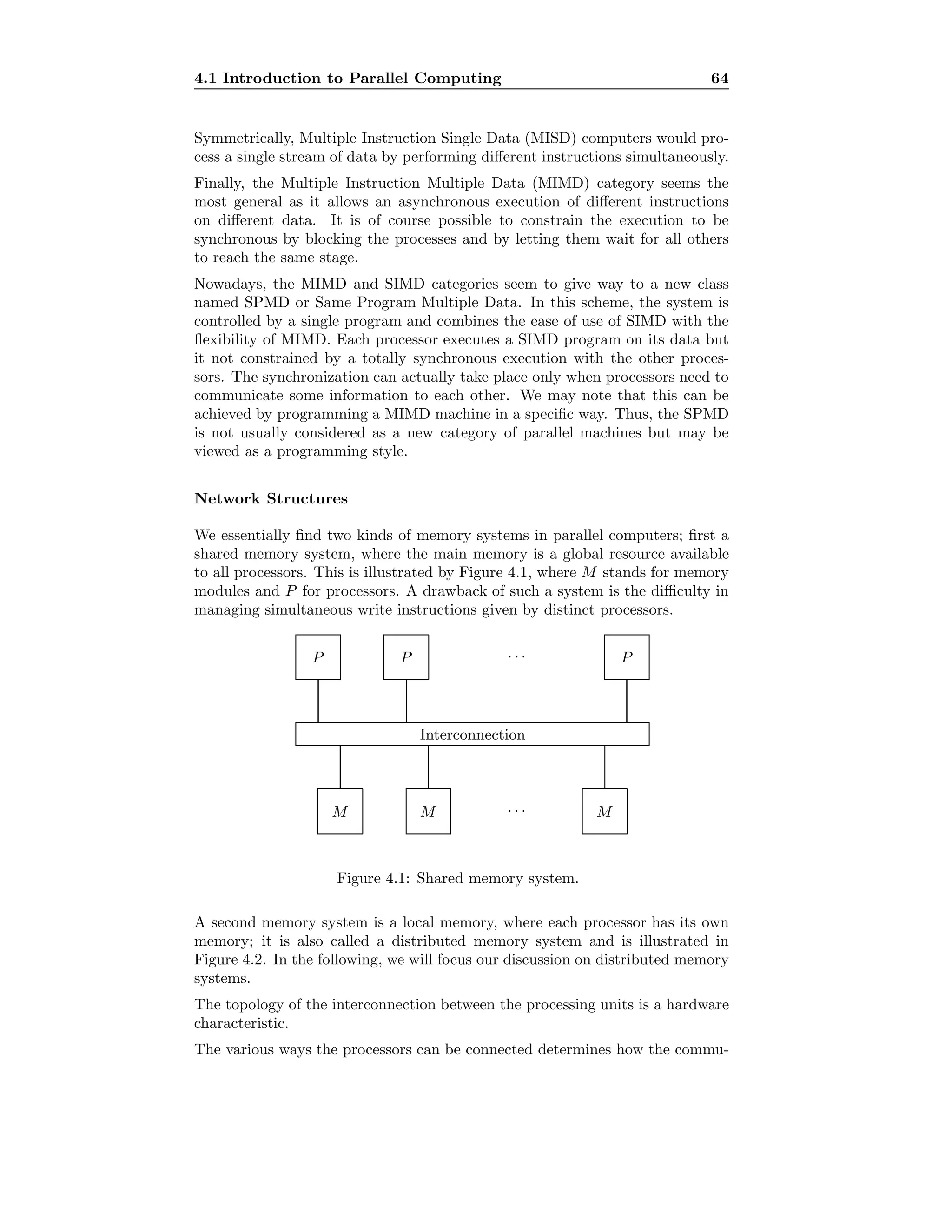


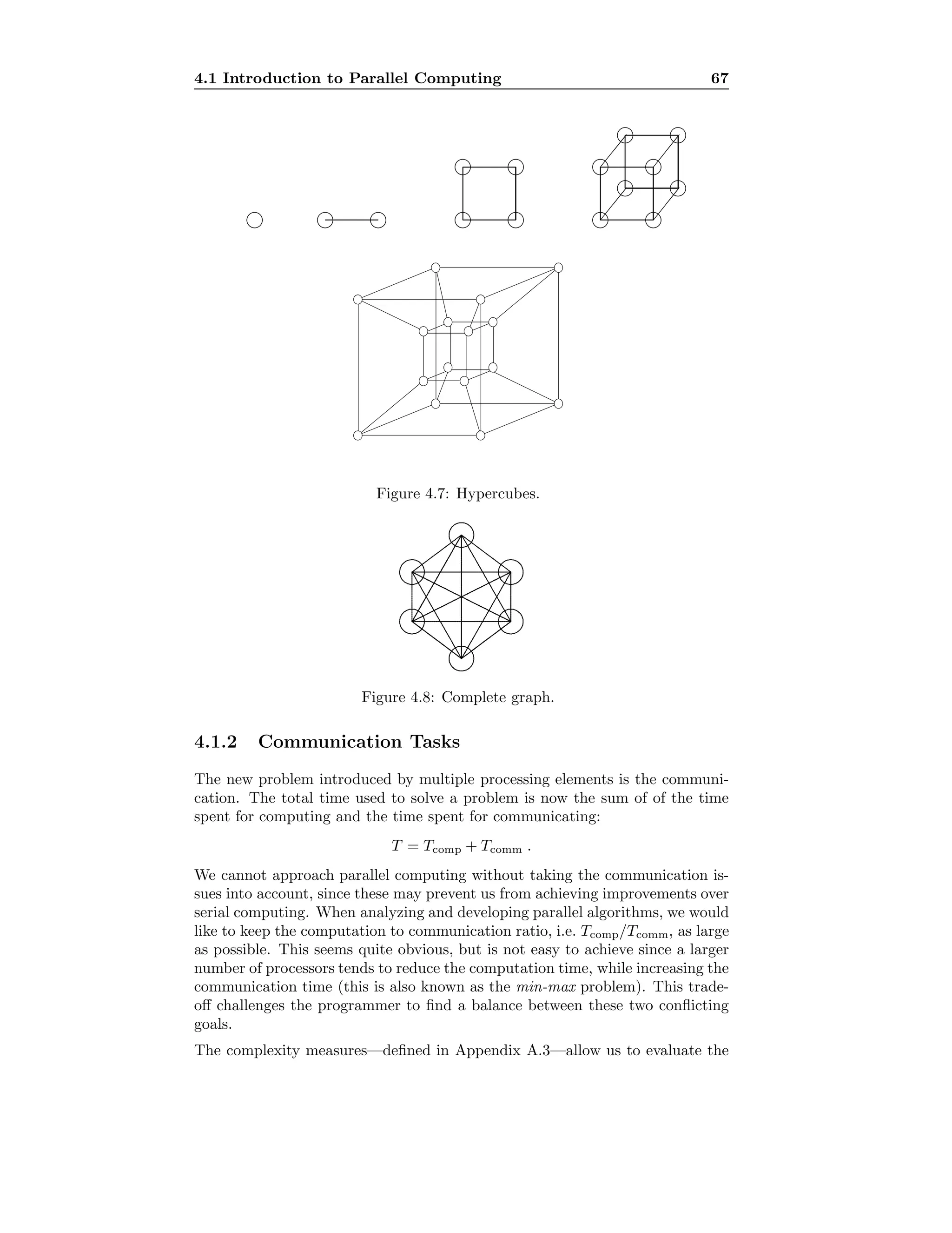

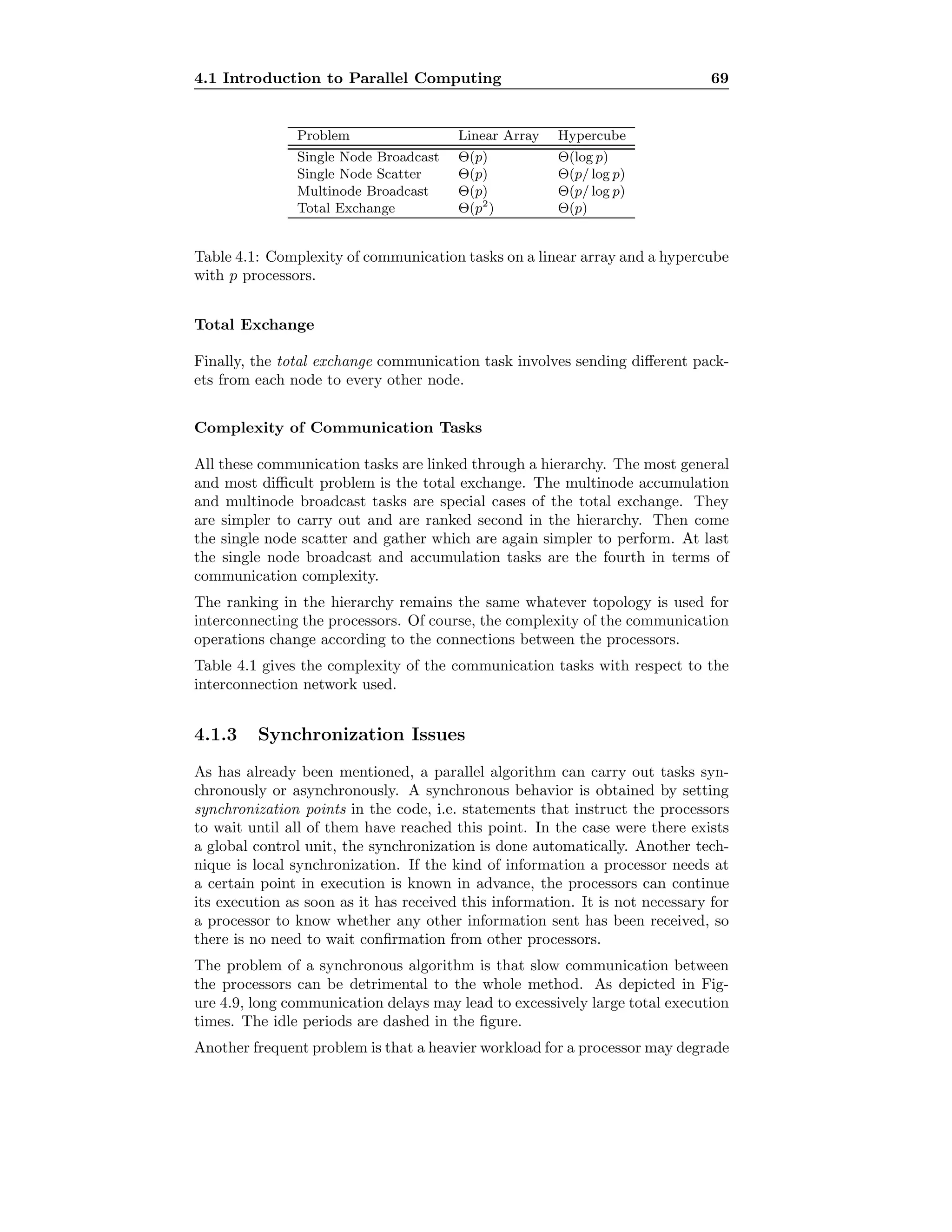

![4.2 Model Simulation Experiences 71
4.2 Model Simulation Experiences
In this section, we will present a practical experience with solution algorithms
executed in a SIMD environment. These results have been published in Gilli
and Pauletto [53] and the presentation closely follows the original paper.
4.2.1 Econometric Models and Solution Algorithms
The econometric models we consider here for solution are represented by a
system of n linear and nonlinear equations
F(y, z) = 0 ⇐⇒ fi(y, z) = 0 , i = 1, 2 . . ., n , (4.1)
where F : Rn
× Rm
→ Rn
is differentiable in the neighborhood of the solution
y∗
∈ Rn
and z ∈ Rm
are the lagged and the exogenous variables. In practice,
the Jacobian matrix DF = ∂F/∂y of an econometric model can often be put
into a blockrecursive form, as shown in Figure 3.1, where the dark shadings
indicate interdependent blocks and the light shadings the existence of nonzero
elements.
The solution of the model then concerns only interdependent submodels. The
approach presented hereafter, applies both to solution of macroeconometric
models and to any large system of nonlinear equations having a structure similar
to the one just described.
Essentially, two types of well-known methods are commonly used for the numer-
ical solution of such systems: first-order iterative techniques and Newton-like
methods. The algorithm have already been introduced as Algorithm 18 and
Algorithm 19 for Jacobi and Gauss-Seidel, and Algorithm 14 for Newton. Here-
after, these algorithms are presented again with slightly different layouts as we
will deal with a normalized system of equations.
First-order Iterative Techniques
The main first-order iterative techniques are the Gauss-Seidel and the Jacobi
iterations.
For these methods, we consider the normalized model as shown in Equation (2.18),
i.e.
yi = gi(y1, . . . , yi−1, yi+1, . . . , yn, z) , i = 1, . . . , n .
In the Jacobi case, the generic iteration k can be written
y
(k+1)
i = gi(y
(k)
1 , . . . , y
(k)
i−1, y
(k)
i+1, . . . , y(k)
n , z) , i = 1, . . . , n (4.2)
and in the Gauss-Seidel case the generic iteration k uses the i − 1 updated
components of the vector y(k+1)
as soon as they are available, i.e.
y
(k+1)
i = gi(y
(k+1)
1 , . . . , y
(k+1)
i−1 , yk
i+1, . . . , y(k)
n , z) , i = 1, . . . , n . (4.3)
In order to be operational the algorithm must also specify a termination criterion
for the iterations. These are stopped if the changes in the solution vector y(k+1)](https://image.slidesharecdn.com/c12cdca8-ad4d-451a-b4fb-6c6bd72ac4d1-161015164104/75/t-79-2048.jpg)

![4.2 Model Simulation Experiences 75
1 1 . . . . . . . . 1 1 1
2 . 1 . . 1 . . 1 . . . .
3 . . 1 . . 1 1 1 . 1 . .
4 . 1 . 1 . . 1 . . 1 . .
5 1 . . 1 1 . . . 1 . . .
6 . 1 . . . 1 1 . . . . .
7 . . . . . . 1 . . 1 . .
8 . 1 . . . . 1 1 . . . .
9 . 1 . . . . . . 1 . 1 .
10 . . 1 . . . . . . 1 . .
11 . 1 . . . . . . . . 1 .
12 1 . . 1 . 1 . . . . . 1
1 2 3 4 5 6 7 8 9 1 1 1
0 1 2
10 1 . . . . . . . . 1 . .
2 . 1 . . 1 . . . . . . 1
7 1 . 1 . . . . . . . . .
11 . 1 . 1 . . . . . . . .
8 . 1 1 . 1 . . . . . . .
6 . 1 1 . . 1 . . . . . .
4 1 1 1 . . . 1 . . . . .
1 1 . . 1 . . . 1 . . 1 .
9 . 1 . 1 . . . . 1 . . .
3 1 . 1 . 1 1 . . . 1 . .
12 . . . . . 1 1 1 . . 1 .
5 . . . . . . 1 1 1 . . 1
1 2 7 1 8 6 4 1 9 3 1 5
0 1 2
level 1
level 2
level 3
level 4
h1
h2
h3
h4
h5
h6
h7
h8 h9
h10
h11
h12
............................................
...........
................................................................................
...........
..............................................................................................................................................................................................................
...........
...............................................................................................................................................
...........
............................................
...........
........................................................................................................................
...........
...............................................................................................................................................
...........
......................................................................... ...........
.............................................
...........
........................................................
...........
........................................................
...........
........................................................
...........
.....................................................................................................................
...........
........................................................
...........
...................................................................................................... ...........
........................................................
...........
........................................................
...........
........................................................
...........
....................................................................................................................................................................................................
...........
...................................................................................................................................................................... ...........
..................................................................................................................................
...........
..............................................
...........
............................................................................. ...........
Figure 4.11: Original and ordered Jacobian matrix and corresponding DAG.
SIMD Computer
A SIMD (Single Instruction Multiple Data) computer usually has a large number
of processors (several thousands), which all execute the same code on different
data sets stored in the processor’s memory. SIMDs are therefore data parallel
processing machines. The central locus of control is a serial computer called
the front end. Neighboring processors can communicate data efficiently, but
general interprocessor communication is associated with a significant loss of
performance.
Single Solution. When solving a model for a single period with the Jacobi or
the Gauss-Seidel algorithm, there are not any possibilities of executing the same
code with different data sets. Only the Newton-like method offers opportunities
for data parallel processing in this situation. This concerns the evaluation of
the Jacobian matrix and the solution of the linear system.4
We notice that the
computations involved in approximating the Jacobian matrix are all indepen-
dent. We particularly observe that the elements of the matrices of order n in
Statements 2 and 4 in Algorithm 23 can be evaluated in a single step with a
speedup of n2
. For a given row i of the Jacobian matrix, we need to evaluate
the function hi for n + 1 different data sets (Statement 3 Algorithm 23). Such
a row can then be processed in parallel with a speedup of n + 1.
4We do not discuss here the fine grain parallelization for the solution of the linear system,
for which we used code from the CMSSL library for QR factorization, see [97].](https://image.slidesharecdn.com/c12cdca8-ad4d-451a-b4fb-6c6bd72ac4d1-161015164104/75/t-83-2048.jpg)
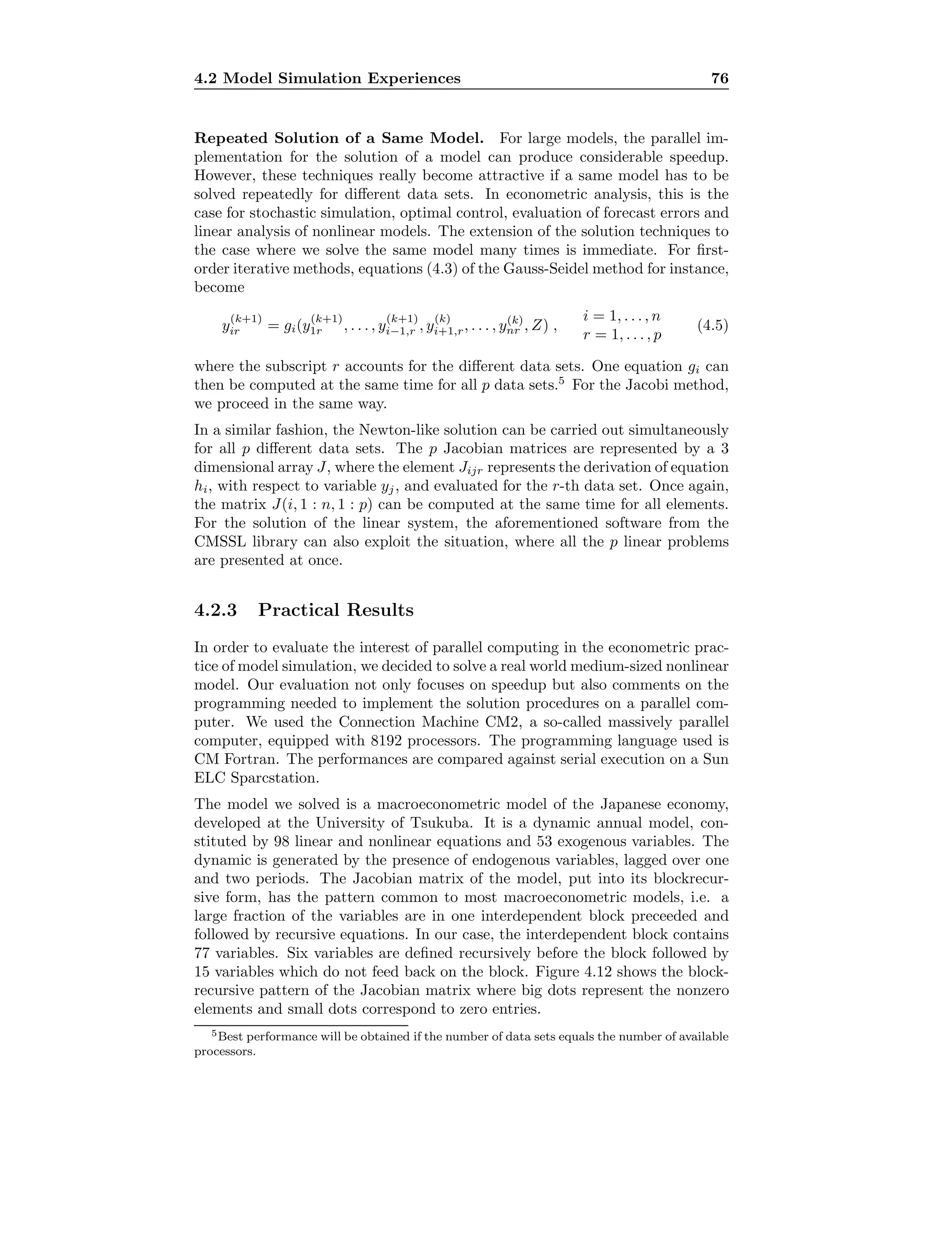
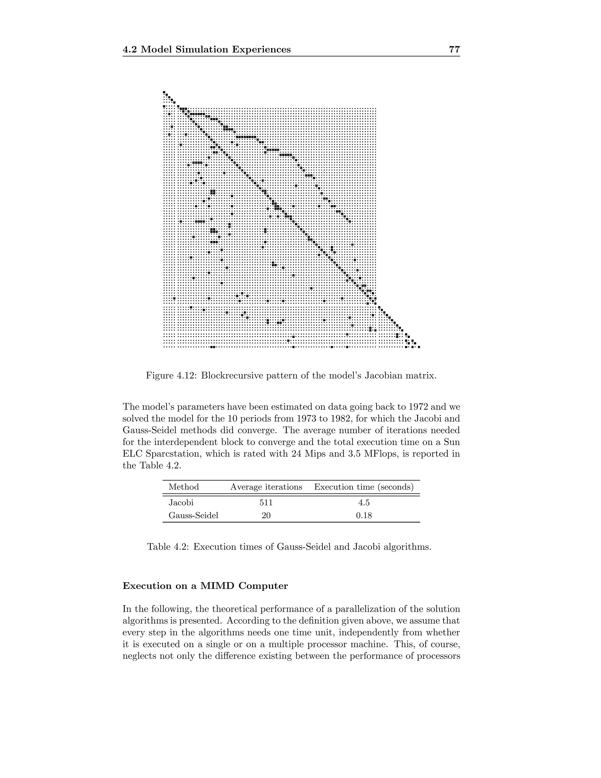
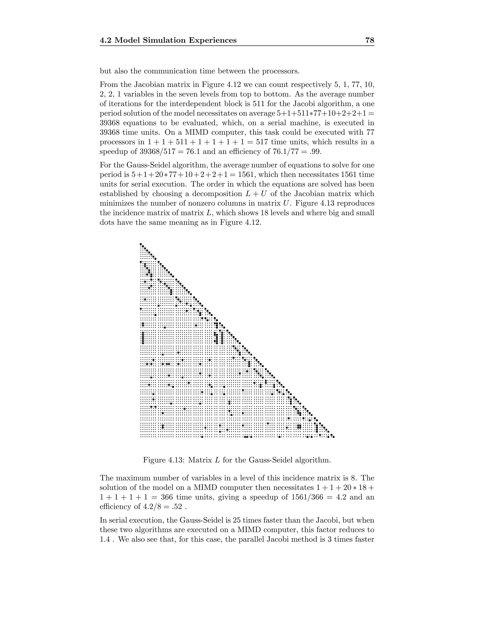
![4.2 Model Simulation Experiences 79
than the serial Gauss-Seidel method, which means that we might be able to
solve problems with the Jacobi method in approximatively the same amount of
time as with a serial Gauss-Seidel method.
If the model’s size increases, the solution on MIMD computers becomes more
and more attractive. For the Jacobi method, the optimum is obviously reached
if the number of equations in a level equals the number of available processors.
For the Gauss-Seidel method, we observe that the ratio between the size of
matrix L and the number of its levels has a tendency to increase for larger
models. We computed this ratio for two large macroeconometric models, MPS
and RDX2.6
For the MPS model, the largest interdependent block is of size 268
and has 28 levels, giving a ratio of 268/28 = 9.6 . For the RDX2 model, this
ratio is 252/40 = 6.3 .
Execution on a SIMD Computer
The situation where we solve repeatedly the same model is ideal for the CM2
SIMD computer. Due to the array-processing features implemented in CM
FORTRAN, which naturally map onto the data parallel architecture7
of the
CM2, it is very easy to get an efficient parallelization for the steps in our algo-
rithms which concern the evaluation of the model’s equations, as it is the case
in Statement 2 in Figure 22 for the first-order algorithms.
Let us consider one of the equations of the model, which, coded in FORTRAN
for a serial execution, looks like
y(8) = exp(b0 + b1 ∗ y(15) + b3 ∗ log(y(12) + b4 ∗ log(y(14))) .
If we want to perform p independent solutions of our equation, we define the
vector y to be a two-dimensional array y(n,p), where the second dimension
corresponds to the p different data sets. As CM FORTRAN treats arrays as
objects, the p evaluations for the equation given above, is simply coded as
follows:
y(8, :) = exp(b0 + b1 ∗ y(15, :) + b3 ∗ log(y(12, :) + b4 ∗ log(y(14, :)))
and the computations to evaluate the p components of y(8,:) are then executed
on p different processors at once.8
To instruct the compiler that we want the p
different data sets, corresponding to the columns of matrix y in the memories
of p different processors we use a compiler directive.9
Repeated solutions of the model have then been experienced in a sensitivity
analysis, where we shocked the values of some of the exogenous variables and
observed the different forecasts. The empirical distribution of the forecasts then
6See Helliwell et al. [63] and Brayton and Mauskopf [19].
7The essence of the CM system is that it stores array elements in the memories of separate
processors and operates on multiple elements at once. This is called data parallel processing.
For instance, consider a n×m array B and the statement B=exp(B). A serial computer would
execute this statement in nm steps. The CM machine, in contrast, provides a virtual processor
for each of the nm data elements and each processor needs to perform only one computation.
8The colon indicates that the second dimension runs over all columns.
9The statement layout y(:serial,:news) instructs the compiler to lay out the second
dimension of array y across the processors.](https://image.slidesharecdn.com/c12cdca8-ad4d-451a-b4fb-6c6bd72ac4d1-161015164104/75/t-87-2048.jpg)
![4.2 Model Simulation Experiences 81
subset of spike variables. However, the cardinality of the set of spike variables
for the interdependent block is five and a comparison of the execution times for
such a small problem would be meaningless. Therefore, we solved the complete
interdependent block without any decomposition, which certainly is not a good
strategy.12
The execution time concerning the main steps of the Newton-like
algorithm needed to solve the model for ten periods is reported in Table 4.4.
Seconds
Statements Sun CM2
2. X = hI + ι y0
0.27 0.23
3. for i = 1 : n, evaluate aij = fi(x.j, z), j = 1 : n and fi(y0
, z) 2.1 122
4. J = (A − ι F(y0
, z) )/h 1.1 0.6
5. solve J s = F(y0
, z) 19.7 12
Table 4.4: Execution time on Sun ELC and CM2 for the Newton-like algorithm.
In order to achieve the numerical stability of the evaluation of the Jacobian ma-
trix, Statements 2, 3 and 4 have to be computed in double precision. Unfortu-
nately, the CM2 hardware is not designed to execute such operations efficiently,
as the evaluation of an arithmetic expression in double precision is about 60
times slower as the same evaluation in single precision. This inconvenience does
not apply to the CM200 model. By dividing the execution time for Statement 3
by a factor of 60, we get approximatively the execution time for the Sun. Since
the Sun processor is about 80 times faster than a processor on the CM2 and
since we have to compute 78 columns in parallel, we therefore just reached the
point from which the CM200 would be faster. Statements 2 and 4 operate on
n2
elements in parallel and therefore their execution is faster on the CM2. From
these results, we conclude that the CM2 is certainly not suited for data paral-
lel processing in double precision. However, with the CM200 model significant
speedup will be obtained if the size of the model to be solved becomes superior
to 80.
12This problem has, for instance, been discussed in Gilli et al. [52]. The execution time for
the Newton method can therefore not be compared with the execution time for the first-order
iterative algorithms.](https://image.slidesharecdn.com/c12cdca8-ad4d-451a-b4fb-6c6bd72ac4d1-161015164104/75/t-89-2048.jpg)
![Chapter 5
Rational Expectations
Models
Nowadays, many large-scale models explicitly include forward expectation vari-
ables that allow for a better accordance with the underlying economic theory
and also provide a response to the Lucas critique. These ongoing efforts gave
rise to numerous models currently in use in various countries. Among others,
we may mention MULTIMOD (Masson et al. [79]) used by the International
Monetary Fund and MX-3 (Gagnon [41]) used by the Federal Reserve Board in
Washington; model QPM (Armstrong et al. [5]) from the Bank of Canada; model
Quest (Brandsma [18]) constructed and maintained by the European Commis-
sion; models MSG and NIGEM analyzed by the Macro Modelling Bureau at the
University of Warwick.
A major technical issue introduced by forward-looking variables is that the sys-
tem of equations to be solved becomes much larger than in the case of conven-
tional models. Solving rational expectation models often constitutes a challenge
and therefore provides an ideal testing ground for the solution techniques dis-
cussed earlier.
5.1 Introduction
Before the more recent efforts to explicitly model expectations, macroeconomic
model builders have taken into account the forward looking behavior of agents
by including distributed lags of the variables in their models. This actually
comes down to supposing that individuals predict a future or current variable
by only looking at past values of the same variable. Practically, this explains
economic behavior relatively well if the way people form their expectations does
not change.
These ideas have been explored by many economists, which has lead to the
so-called “adaptive hypothesis.” This theory states that the individual’s expec-
tations react to the difference between actual values and expected values of the
variable in question. If the level of the variable is not the same as the forecast,](https://image.slidesharecdn.com/c12cdca8-ad4d-451a-b4fb-6c6bd72ac4d1-161015164104/75/t-90-2048.jpg)
![5.1 Introduction 83
the agents use their forecasting error to revise their expectation of the next
period’s forecast. This setting can be summarized in the following equation1
xe
t − xe
t−1 = λ(xt−1 − xe
t−1) with 0 λ ≤ 1 ,
where xe
t is the forecasted and non observable value of variable x at period t.
By rearranging terms we get
xe
t = λxt−1 + (1 − λ)xe
t−1 ,
i.e. the forecasted value for the current period is a weighted average of the true
value of x at period t − 1 and the forecasted value at period t − 1. Substituting
lagged values of xe
t when λ = 1 in this expression yields to
xe
t = λ
∞
i=1
(1 − λ)i−1
xt−i .
The speed at which the agents adjust is determined by parameter λ.
In this framework, individuals constantly underpredict the value of the vari-
able whenever the variable constantly increases. This behavior is labelled “not
rational” since agents make systematically errors in their expected level of x.
It is therefore argued that individuals would not behave that way since they
can do better. As many other economists, Lucas [77] criticized this assumption
and proposed models consistent with the underlying idea that agents do their
best with the information they have. The “rational expectation hypothesis” is
an alternative which takes into account such criticisms. We assume that indi-
viduals use all information efficiently and do not systematically make errors in
their predictions. Agents use the knowledge they have to form views about the
variables entering their model and produce expectations of the variables they
want to use to make their decisions.
This role of expectations in economic behavior has been recognized for a long
time. The explicit use of the term “rational expectations” goes back to the work
of Muth in 1961 as reprinted in Lucas and Sargent [75]. The rational expec-
tations are the true mathematical expectations of future and current variables
conditional on the information set available to the agents. This information set
at date t − 1 contains all the data on the variables of the model up to the end
of period t − 1, as well as the relevant economic model itself.
The implications of the rational expectation hypothesis is that the policies the
government may try to impose are ineffective since agents forecast the change
in the variables using the same information basis. Even in the short term,
systematic interventions of monetary or fiscal policies only affect the general
level of prices but not the real output or employment.
A criticism often made against this hypothesis is that obtaining the information
is costly and therefore not all information may be used by the agents. Moreover
not all agents may build a good model to reach their forecasts. An answer to
these points is that even if not all individuals are well informed and produce
good predictions, some individuals will. An arbitrage process can therefore
1The model is sometimes expressed as xe
t − xe
t−1 = λ(xt − xe
t−1) . In this case, the expec-
tation formation is somewhat different but the conclusions are similar for our purposes.](https://image.slidesharecdn.com/c12cdca8-ad4d-451a-b4fb-6c6bd72ac4d1-161015164104/75/t-91-2048.jpg)
![5.1 Introduction 84
take place and the agents who have the correct information can make profits
by selling the information to the ill-informed ones. This process will lead the
economy to the rational expectation equilibrium.
Fair [33] summarizes the main characteristics of rational expectation (RE) mod-
els such as those of Lucas [76], Sargent [91] and Barro [9] in the three following
points,
• the assumption that expectations are rational, i.e. consistent with the
model,
• the assumption that information is imperfect regarding the current state
of the economy,
• the postulation of an aggregate supply equation in which aggregate supply
is a function of exogenous terms plus the difference between the actual and
the expected price level.
These characteristics imply that government actions have an influence on the
real output only if these actions are unanticipated. The second assumption
allows for an effect of government actions on the aggregate supply since the
difference between the actual and expected price levels may be influenced. A
systematic policy is however anticipated by the agents and cannot affect the
aggregate supply.
One of the key conclusions of new-classical authors is that existing macroecono-
metric models were not able to provide guidance for economic policy.
This critique has lead economists to incorporate expectations in the relationships
of small macroeconomic models as Sargent [92] and Taylor [96]. By now this
idea has been adopted as a part of new-classical economics.
The introduction of the rational expectation hypothesis opened new research
topics in econometrics that has given rise to important contributions. According
to Beenstock [12, p. 141], the main issues of the RE hypothesis are the following:
• Positive economics, i.e. what are the effects of policy interventions if ra-
tional expectations are assumed?
• Normative economics, i.e. given that expectations are rational, ought the
government take policy actions?
• Hypothesis testing, i.e. does evidence in empirical studies support the
rational expectations hypothesis? Are such models superior to others
which do not include this hypothesis?
• Techniques, i.e. how does one solve a model with rational expectations?
What numerical issues are faced? How can we efficiently solve large models
with forward-looking variables?
These problems, particularly the first three, have been addressed by many au-
thors in the literature.
New procedures for estimation of the model’s parameters were set forth in Mc-
Callum [80], Wallis [101], Hansen and Sargent [62], Wickens [102], Fair and](https://image.slidesharecdn.com/c12cdca8-ad4d-451a-b4fb-6c6bd72ac4d1-161015164104/75/t-92-2048.jpg)
![5.1 Introduction 85
Taylor [34] and Nijman and Palm [84]. The presence of forward looking vari-
ables also creates a need for new solution techniques for simulating such models,
see for example Fair and Taylor [34], Hall [61], Fisher and Hughes Hallett [37],
Laffargue [74] and Boucekkine [17].
In the next section, we introduce a formulation of RE models that will be used
to analyze the structure of such models. A second section discusses issues of
uniqueness and stability of the solutions.
5.1.1 Formulation of RE Models
Using the conventional notation (see for instance Fisher [36]) a dynamic model
with rational expectations is written
fi(yt, yt−1, . . . , yt−r, yt+1|t−1, . . . , yt+h|t−1, zt) = 0 , i = 1, . . . , n , (5.1)
where yt+j|t−1 is the expectation of yt+j conditional on the information avail-
able at the end of period t − 1, and zt represents the exogenous and random
variables. For consistent expectations, the forward expectations yt+j|t−1 have
to coincide with the next period’s forecast when solving the model conditional
on the information available at the end of period t − 1. These expectations are
therefore linked forward in time and, solving model (5.1) for each yt conditional
on some start period 0 requires each yt+j|0, for j = 1, 2, . . . , T −t, and a terminal
condition yT +j|0, j = 1, . . . , h.
We will now consider that the system of equations contains one lag and one
lead, that is, we set r = 1 and h = 1 in (5.1) so as to simplify notation. In
order to discuss the structure of our system of equations, it is also convenient
to resort to a linearization. System (5.1) becomes therefore
Dt
yt + Et−1
yt−1 + At+1
yt+1|t−1 = zt (5.2)
where we have Dt
= ∂f
∂yt
, Et−1
= − ∂f
∂yt−1
and At+1
= − ∂f
∂yt+1|t−1
. Stacking up
the system for period t + 1 to period t + T we get
Et+0
Dt+1
At+2
Et+1
Dt+2
At+3
...
...
...
Et+T −2
Dt+T −1
At+T
Et+T −1
Dt+T
At+T +1
yt+0
yt+1
yt+2
...
yt+T −1
yt+T
yt+T +1
=
zt+1
zt+2
...
zt+T −1
zt+T
(5.3)
and a consistent expectations solution to (5.3) is then obtained by solving
Jy = b ,](https://image.slidesharecdn.com/c12cdca8-ad4d-451a-b4fb-6c6bd72ac4d1-161015164104/75/t-93-2048.jpg)
![5.1 Introduction 86
where J is the boxed matrix in Equation (5.3), y = [yt+1 . . . yt+T ] and
b =
zt+1
...
zt+T
+
−Et+0
...
0
yt+0 +
0
...
−At+T +1
yt+T +1
are the stacked vectors of endogenous respectively exogenous variables which
contain the initial condition yt+0 and the terminal conditions yt+T +1.
5.1.2 Uniqueness and Stability Issues
To study the dynamic properties of RE models, we begin with the standard pre-
sentation of conventional models containing only lagged variables. The struc-
tural form of the general linear dynamic model is usually written as
B(L)yt + C(L)xt = ut ,
where B(L) and C(L) are matrices of polynomials in the lag operator L and ut
a vector of error terms. The matrices are respectively of size n × n and n × g,
where n is the number of endogenous variables and g the number of exogenous
variables, and defined as
B(L) = B0 + B1L + · · · + BrLr
, C(L) = C0 + C1L + · · · + CsLs
.
The model is generally subject to some normalization rule i.e. diag(B0) =
[1 1 . . . 1]. The dynamic of the model is stable if the determinantal polyno-
mial |B(z)| = det(
r
j=0 Bjzj
) has all its roots λi , i = 1, 2, . . . , nr outside the
unit circle. The endogenous variables yt can be expressed as
yt = −B(L)−1
C(L)xt + B(L)−1
ut . (5.4)
Assuming the stability of the system, the distributed lag on the exogenous vari-
ables xt is non-explosive. If there exists at least one root with modulus less than
unity, the solution for yt is explosive. Wallis [100] writes Equation (5.4) using
|B(L)| the determinant of the matrix polynomial B(L) and b(L) the adjoint
matrix of B(L)
yt = −
b(L)
|B(L)|
C(L)xt +
b(L)
|B(L)|
ut . (5.5)
To study stability, let us write the following polynomial in factored form
|B(z)| =
nr
i=1
βizi
= βnr
nr
i=1
(z − λi) , (5.6)
where λi , i = 1, 2, . . . , nr are the roots of |B(z)| and βnr is the coefficient of
the term znr
. Assuming βnr = 0, the polynomial defined in (5.6) has the same
roots as the polynomial
nr
i=1
(z − λi) . (5.7)](https://image.slidesharecdn.com/c12cdca8-ad4d-451a-b4fb-6c6bd72ac4d1-161015164104/75/t-94-2048.jpg)
![5.1 Introduction 87
When β1 = 0, none of the λi , i = 1, . . . , nr can be zero. Therefore, we may
express a polynomial with the same roots as (5.7) by the following expression
nr
i=1
(1 −
z
λi
) =
nr
i=1
(1 − µiz) with µi = 1/λi . (5.8)
Assuming that the model is stable, i.e. that |λi| 1 , i = 1, 2, . . ., nr, we have
that |µi| 1 , i = 1, 2, . . . , nr.
We now consider the expression 1/|B(z)| that arises in (5.5) and develop the
expansion in partial fractions of the ratio of polynomials 1/ (1 − µiz) (the
numerator being the polynomial ‘1’) that has the same roots as 1/|B(z)|:
1
nr
i=1(1 − µiz)
=
nr
i=1
ci
(1 − µiz)
. (5.9)
For a stable root, say |λ| 1 (|µ| 1), the corresponding term of the right
hand side of (5.9) may be expanded into a polynomial of infinite length
1
(1 − µz)
= 1 + µz + µ2
z2
+ · · · (5.10)
= 1 + z/λ + z2
/λ2
+ · · · . (5.11)
This corresponds to an infinite series in the lags of xt in expression (5.5). In the
case of an unstable root, |λ| 1 (|µ| 1), the expansion (5.11) is not defined,
but we can use an alternative expansion as in [36, p. 75]
1
(1 − µz)
=
−µ−1
z−1
(1 − µ−1z−1)
(5.12)
= − λz−1
+ λ2
z−2
+ · · · . (5.13)
In this formula, we get an infinite series of distributed leads in terms of Equa-
tion (5.5) by defining L−1
xt = Fxt = xt+1. Therefore, the expansion is depen-
dent on the future path of xt. This expansion will allow us to find conditions
for the stability in models with forward looking variables.
Consider the model
B0yt + ˜A(F)yt+1|t−1 = C0xt + ut , (5.14)
where for simplicity no polynomial lag is applied to the current endogenous and
exogenous variables. As previously, yt+1|t−1 denotes the conditional expectation
of variable yt+1 given the information set available at the end of period t − 1.
The matrix polynomial in the forward operator F is defined as
˜A(F) = ˜A0 + ˜A1F + · · · + ˜AhFh
,
and has dimensions n×n. The forward operator affects the dating of the variable
but not the dating of the information set so that
Fyt+1|t−1 = yt+2|t−1 .](https://image.slidesharecdn.com/c12cdca8-ad4d-451a-b4fb-6c6bd72ac4d1-161015164104/75/t-95-2048.jpg)
![5.1 Introduction 88
When solving the model for consistent expectations, we set yt+1|t−1 to the so-
lution of the model, i.e. yt+i. In this case, we may rewrite model (5.14) as
A(F)yt = C0xt + ut , (5.15)
with A(F) = B0 + ˜A(F). The stability of the model is therefore governed by
the roots γi of the polynomial |A(z)|. When for all i we have |γi| 1, the
model is stable and we can use an expansion similar to (5.11) to get an infinite
distributed lead on the exogenous term xt. On the other hand, if there exist
unstable roots |γi| 1 for some i, we may resort to expansion (5.13) which
yields an infinite distributed lag.
As exposed in Fisher [36, p. 76], we will need to have |γi| 1 , ∀i in order to
get a unique stable solution. To solve (5.15) for yt+i , i = 1, 2, . . ., T we must
choose values for the terminal conditions yt+T +j , j = 1, 2, . . ., h. The solution
path selected for yt+i , i = 1, 2, . . . , T depends on the values of these terminal
conditions. Different conditions on the yt+T +j , j = 1, 2, . . . , h generate differ-
ent solution paths. If there exists an unstable |γi| 1 for some i, then part
of the solution only depends on lagged values of xt. One may therefore freely
choose some terminal conditions by selecting values of xt+T +j , j = 1, . . . , h,
without changing the solution path. This hence would allow for multiple stable
trajectories. We will therefore usually require the model to be stable in order
to obtain a unique stable path.
The general model includes lags and leads of the endogenous variables and may
be written
B(L)yt + A(F)yt+1|t−1 + C(L)xt = ut ,
or equivalently
D(L, F)yt + C(L) = ut ,
where D(L, F) = B(L)+A(F) and we suppose the expectations to be consistent
with the model solution. Recalling that L = F−1
in our notation, the stability
conditions depend on the roots of the determinantal polynomial |D(z, z−1
)|. To
obtain these roots, we resort to a factorization of matrix D(z, z−1
). When there
is no zero root, we may write
D(z, z−1
) = U(z) W V (z−1
) ,
where U(z) is a matrix polynomial in z, W is a nonsingular matrix and V (z−1
)
is a matrix polynomial in z−1
. The roots of |D(z, z−1
)| are those of |U(z)| and
|V (z−1
)|. Since we assumed that there exists no zero root, we know that if
|V (z−1
)| = v0 + v1z−1
+ · · · + vhz−h
has roots δi , i = 1, . . . , h then | ˜V (z)| =
vh + vh−1z + · · · + v0zh
has roots 1/δi , i = 1, . . . , h. The usual stability
condition is that |U(z)| and | ˜V (z)| must have roots outside the unit circle.
This, therefore, is equivalent to saying that |U(z)| has roots in modulus greater
than unity, whereas |V (z−1
)| has roots less than unity.
With these conditions, the model must have as many unstable roots as there are
expectation terms, i.e. h. In this case, we can define infinite distributed lags and
leads that allow the selection of a unique stable path of yt+j , j = 1, 2, . . ., T
given the terminal conditions.](https://image.slidesharecdn.com/c12cdca8-ad4d-451a-b4fb-6c6bd72ac4d1-161015164104/75/t-96-2048.jpg)
![5.2 The Model MULTIMOD 89
5.2 The Model MULTIMOD
In this section, we present the model we used in our solution experiments. First,
a general overview of the model is given in Section 5.2.1; then, the equations that
compose an industrialized country are presented in Section 5.2.2. Section 5.2.3
briefly introduces the structure of the complete model.
5.2.1 Overview of the Model
MULTIMOD (Masson et al. [79]) is a multi-region econometric model developed
by the International Monetary Fund in Washington. The model is available upon
request and is therefore widely used for academic research.
MULTIMOD is a forward-looking dynamic annual model and describes the eco-
nomic behavior of the whole world decomposed into eight industrial zones and
the rest of the world. The industrial zones correspond to the G7 and a zone
called “small industrial countries” (SI), which collects the rest of the OECD. The
rest of the world comprises two developing zones, i.e. high-income oil exporters
(HO) and other developing countries (DC). The model mainly distinguishes
three goods, which are oil, primary commodities and manufactures. The short-
run behavior of the agents is described by error correction mechanisms with
respect to their long-run theory based equilibrium. Forward-looking behavior is
modeled in real wealth, interest rates and in the price level determination.
The specification of the models for industrialized countries is the same and
consists of 51 equations each. These equations explain aggregate demand, taxes
and government expenditures, money and interest rates, prices and supply, and
international balances and accounts.
Consumption is based on the assumption that households maximize the dis-
counted utility of current and future consumption subject to their budget con-
straint. It is assumed that the function is influenced by changes in disposable
income wealth and real interest rates. The demand for capital follows Tobin’s
theory, i.e. the change in the net capital stock is determined by the gap between
the value of existing capital and its replacement cost. Conventional import and
export functions depending upon price and demand are used to model trade.
This makes the simulation of a single country model meaningful. Trade flows for
industrial countries are disaggregated into oil, manufactured goods and primary
commodities. Government intervention is represented by public expenditures,
money supply, bonds supply and taxes. Like to most macroeconomic models,
MULTIMOD describes the LM curve by conventional demand for money bal-
ances and a money supply consisting in a reaction function of the short-term
interest rate to a nominal money target, except for France, Italy and the smaller
industrial countries where it is assumed that Central Banks move short-term
interest rates to limit movements of their exchange rates with respect to the
Deutsche Mark. The aggregate supply side of the model is represented by an in-
flation equation containing the expected inflation rate. A set of equation covers
the current account balance, the net international asset or liability position and
the determination of exchange rates.
As already mentioned, the rest of the world is aggregated into two regions, i.e.](https://image.slidesharecdn.com/c12cdca8-ad4d-451a-b4fb-6c6bd72ac4d1-161015164104/75/t-97-2048.jpg)

![5.3 Solution Techniques for RE Models 93
0 100 200 300 400
0
50
100
150
200
250
300
350
400
450
nz = 2260
Figure 5.2: Incidence matrix of D in MULTIMOD.
An alternative approach presented in Section 5.3.2 consists in stacking up the
equations for a given number of time periods. In such a case, it is necessary to
explicitly specify terminal conditions for the system. This system can then be
either solved with a block iterative method or a Newton-like method. The com-
putation of the Newton step requires the solution of a linear system for which we
consider different solution techniques in Section 5.3.4. Section 5.3.3 introduces
block iterative schemes and possibilities of parallelization of the algorithms.
5.3.1 Extended Path
Fair’s and Taylor’s extended path method (EP) [34] constitutes the first oper-
ational approach to the estimation and solution of dynamic nonlinear rational
expectation models.
The method does not require the setting of terminal conditions as explained in
Section 5.1.1. In the case where terminal conditions are known, the method
does not need type III iterations and the correct answer is found after type II
iterations converged.
The method can be described as follows:
1. Choose an integer k as an initial guess for the number of periods beyond
the horizon h for which expectations need to be computed to obtain a
solution within a prescribed tolerance.
Choose initial values for yt+1|t−1, . . . , yt+2h+k|t−1.
2. Solve the model dynamically to obtain new values for the variables
yt+1|t−1, . . . , yt+h+k|t−1 .
Fair and Taylor suggest using Gauss-Seidel iterations to solve the model.
(Type I iterations).
3. Check the vectors yt+1|t−1, . . . , yt+h+k|t−1 for convergence. If any of these
values have not converged, go to step 2. (Type II iterations).](https://image.slidesharecdn.com/c12cdca8-ad4d-451a-b4fb-6c6bd72ac4d1-161015164104/75/t-101-2048.jpg)
![5.3 Solution Techniques for RE Models 94
4. Check the set of vectors yt+1|t−1, . . . , yt+h+k|t−1 for convergence with the
same set that most recently reached this step. If the convergence criterion
is not satisfied, then extend the solution horizon by setting k to k + 1 and
go to step 2. (Type III iterations).
5. Use the computed values of yt+1|t−1, . . . , yt+h+k|t−1 to solve the model for
period t.
The method treats endogenous leads as predetermined, using initial guesses,
and solves the model period by period over some given horizon. This solution
produces new values for the forward-looking variables (leads). This process is
repeated until convergence of the system. Fair and Taylor call these iterations
“type II iterations” to distinguish them from the standard “type I iterations”
needed to solve the nonlinear model within each time period. The type II
iterations generate future paths of the expected endogenous variables. Finally,
in a “type III iteration”, the horizon is augmented until this extension does not
affect the solution within the time range of interest.
Algorithm 25 Fair-Taylor Extended Path Method
Choose k and initial values yi
t+r , r = 1, 2, . . . , k + 2h , i = I, II, III
repeat until [yIII
t yIII
t+1 . . . yIII
t+h] converged
repeat until [yII
t yII
t+1 . . . yII
t+h+k] converged
for i = t, t + 1, . . . , t + h + k
repeat until yI
i converged
set yII
i = yI
i
end
end
set [yIII
t . . . yIII
t+h] = [yII
t . . . yII
t+h]
k = k + 1
end
5.3.2 Stacked-time Approach
An alternative approach consists in stacking up the equations for successive time
periods and considering the solution of the system written in Equation (5.3).
According to what has been said in Section 3.1, we first begin to analyze the
structure of the incidence matrix of J, which is
J =
D A 0 · · · 0
E D A · · · 0
0 E D · · · 0
...
...
...
0 · · · D
,
where we have dropped the time indices as the incidence matrices of Et+j
, Dt+j
and At+j
j = 1, . . . , T are invariant with respect to j.
As matrix D, and particularly matrices E and A are very sparse, it is likely that
matrix J can be rearranged into a blocktriangular form J∗
. We know that as a
consequence it would then be possible to solve parts of the model recursively.](https://image.slidesharecdn.com/c12cdca8-ad4d-451a-b4fb-6c6bd72ac4d1-161015164104/75/t-102-2048.jpg)

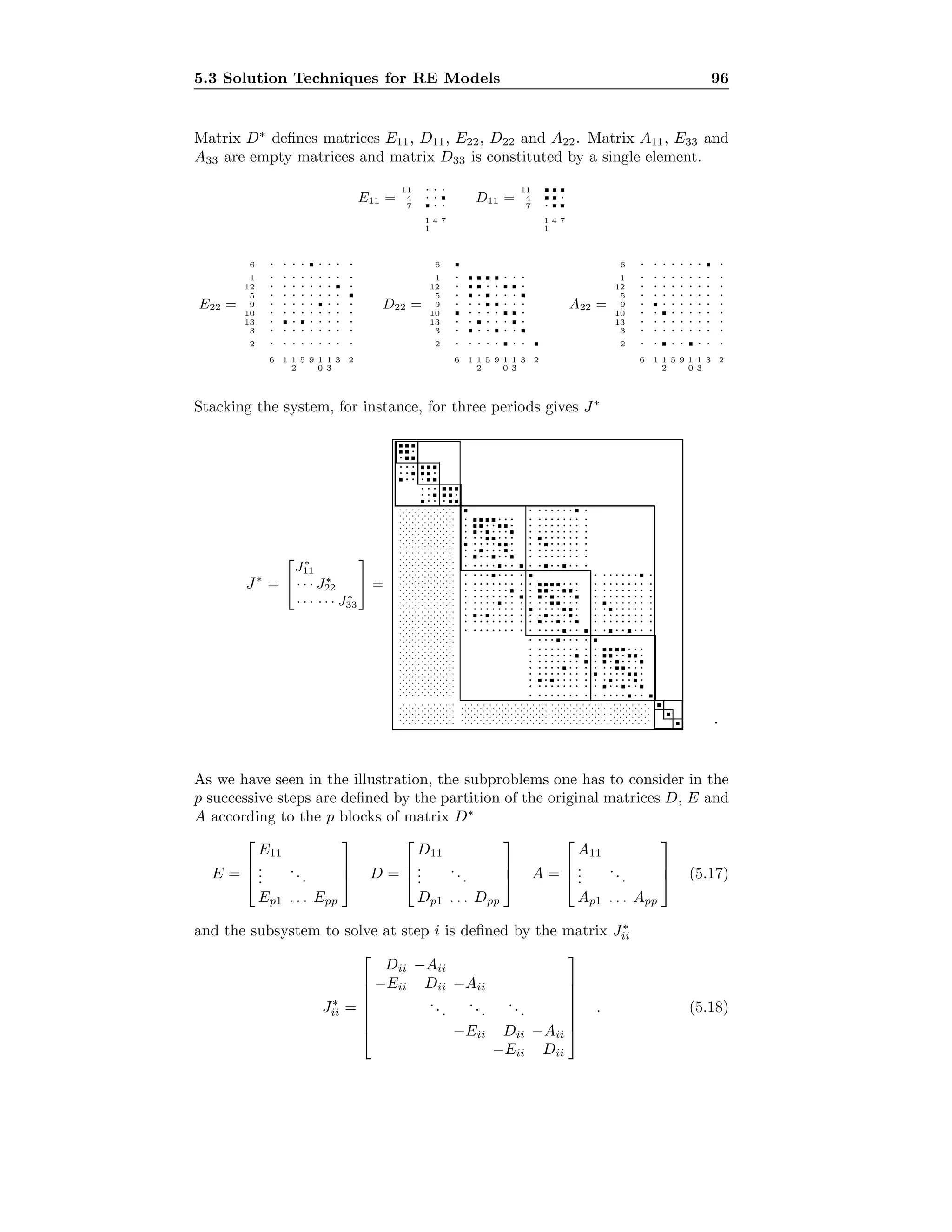
![5.3 Solution Techniques for RE Models 97
It is clear that for the partition given in (5.17), some of the submatrices Dii are
likely to be decomposable and some of the matrices Eii and Aii will be zero.
As a consequence, matrix J∗
ii can have different kinds of patterns according
to whether the matrices Eii and Aii are zero or not. These situations are
commented hereafter.
If matrix Aii ≡ 0, we have to solve a blockrecursive system which corresponds
to the solution of a conventional dynamic model (case of J∗
11 in our example). In
practice, this corresponds to a separable submodel for which there do not exist
any forward looking mechanisms. As a special case, the system can be com-
pletely recursive if Dii is of order one, or a sequence of independent equations
or blocks if Eii ≡ 0. This is the case of J∗
33 in our example.
In the case where matrix Aii ≡ 0 and Eii ≡ 0 as for J∗
22 in our example, we
have to solve an interdependent system. In practice, we often observe that
a large part of the equations are contained in one block Dii, for which the
corresponding matrix Aii is nonzero, and one might think that little is gained
with such a decomposition. However, even if the size of the blockrecursive part
is relatively small compared to the rest of the model, this decomposition is
nevertheless useful, as in some problems the number of periods T for which we
have to stack the model can go into the order of hundreds. The savings in term
of size of the interdependent system to be solved may therefore not be negligible.
From this point onwards in our work, we will consider the solution of an inde-
composable system of equations defined by J∗
ii.
5.3.3 Block Iterative Methods
We now consider the solution of a given system J∗
ii and denote by y = [y1 . . . yT ]
the array corresponding to the stacked vectors for T periods. In the following we
will use dots to indicate subarrays. For instance, y·t designates the t-th column
of array y.
A block iterative method for solving an indecomposable J∗
ii, consists in executing
K loops over the equations of each period. For K = 1, we have a point method
and, for an arbitrary K, the algorithm is formalized in Algorithm 26.
Algorithm 26 Incomplete Inner Loops
repeat until convergence
1. for t = 1 to T
2. for k = 1 to K
3. y0
·t = y1
·t
4. for i = 1 to n
5. Evaluate y1
it
end
end
end
end
Completely solving the equations for each period constitutes a particular case
of this algorithm. In such a situation, we execute the loop over k until the](https://image.slidesharecdn.com/c12cdca8-ad4d-451a-b4fb-6c6bd72ac4d1-161015164104/75/t-105-2048.jpg)
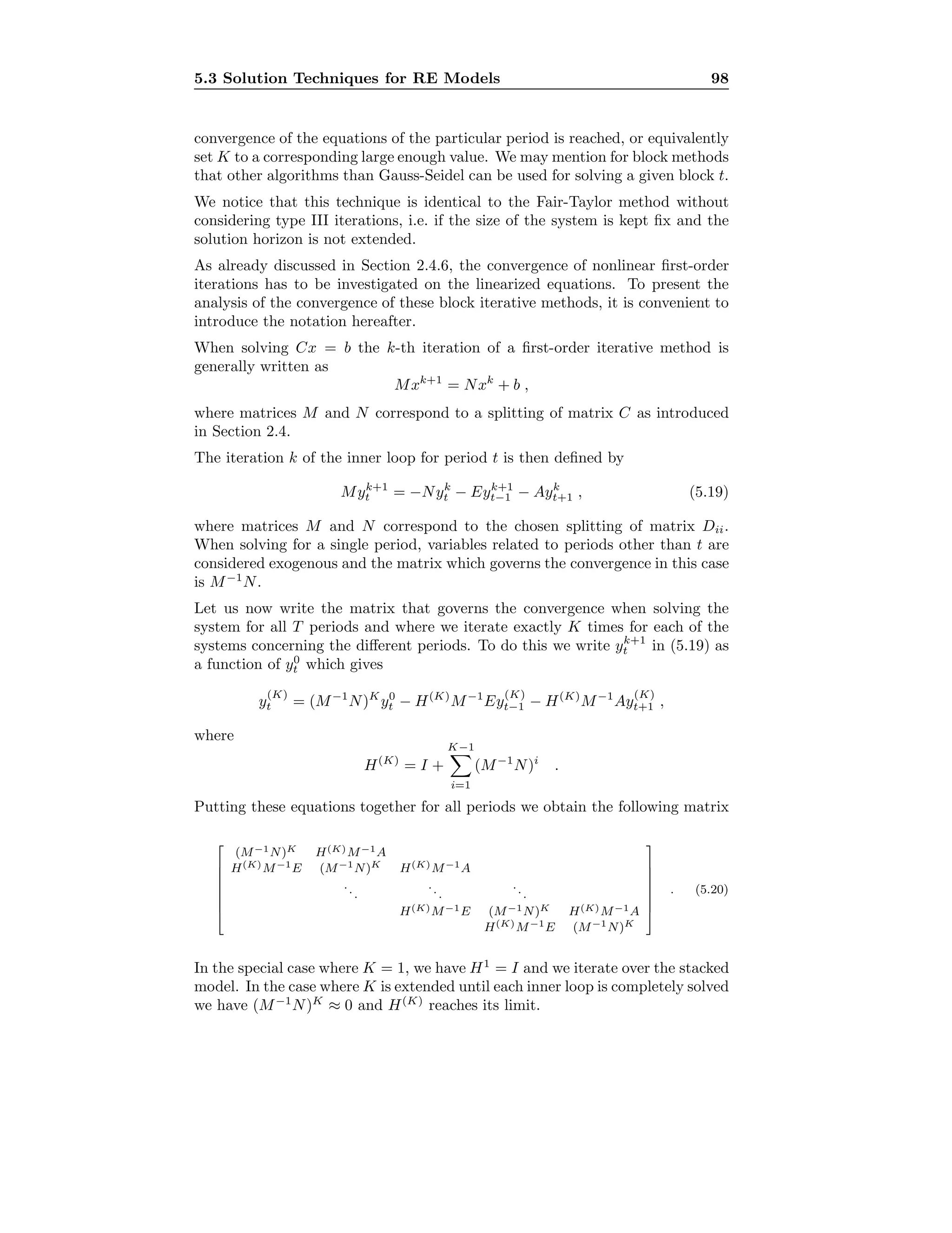
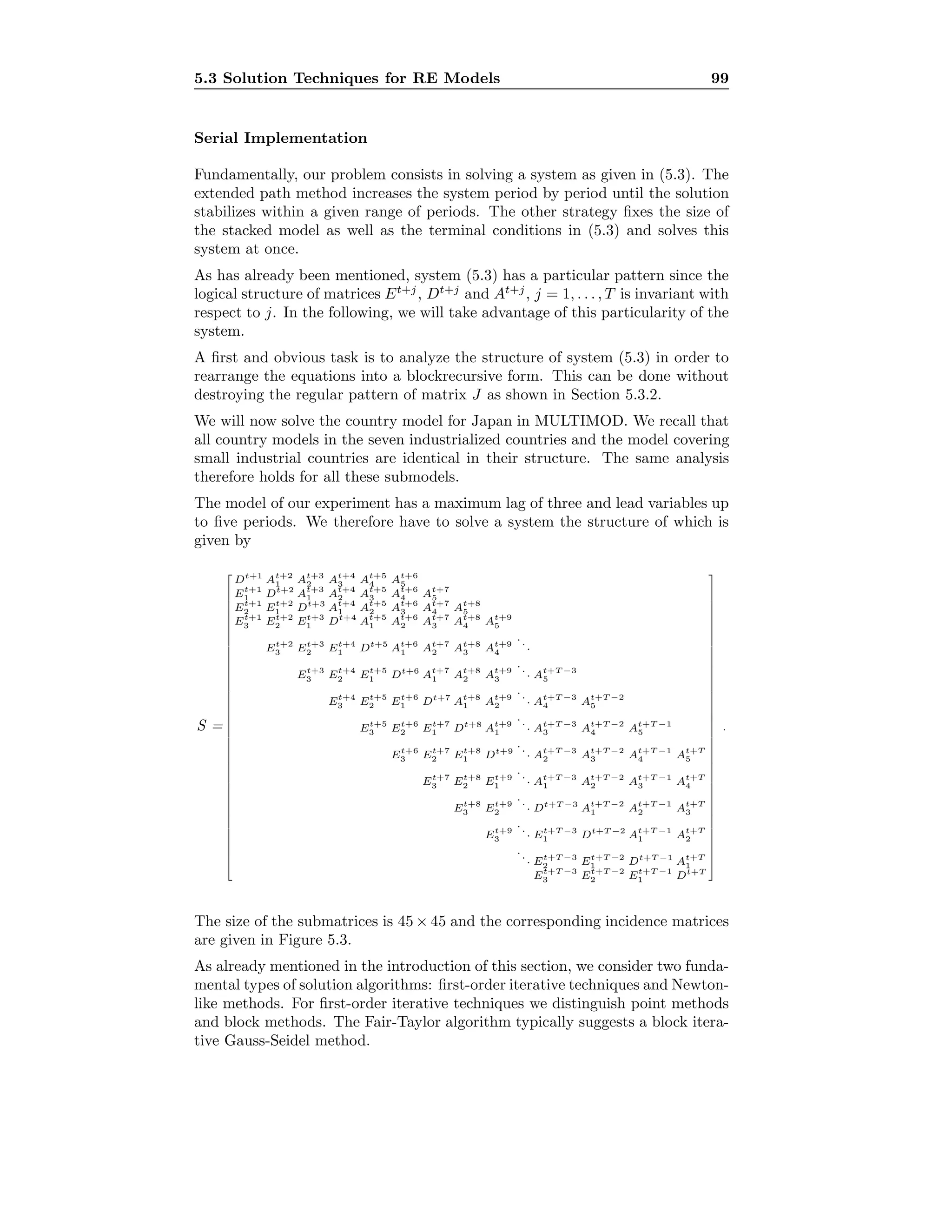
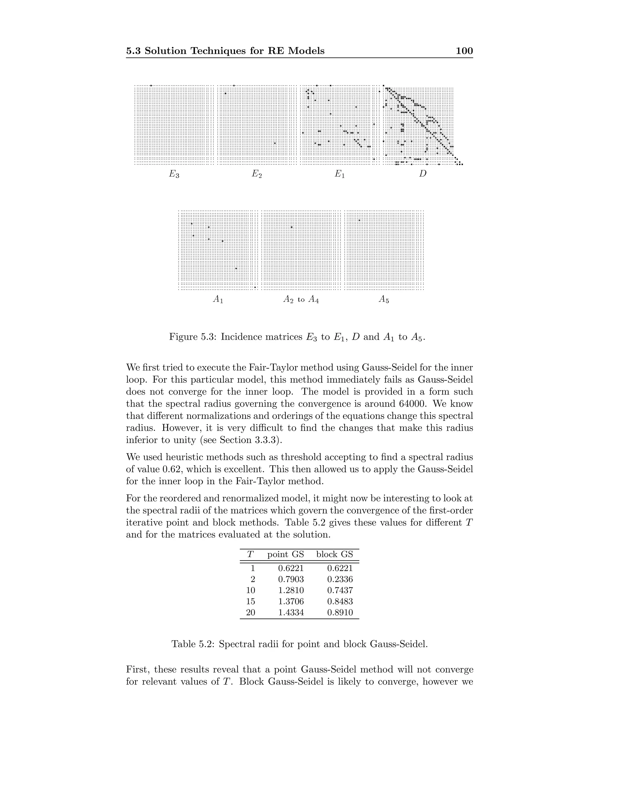

![5.3 Solution Techniques for RE Models 102
Algorithm 28 Parallel Simulations
while not converged
1. y0
= y1
2. for i = 1 to n
3. for t = 1 to T and s = 1 to S in parallel do
4. Evaluate y1
its
end
end
end
With the array-processing features, as implemented for instance in High Per-
formance Fortran [66], it is very easy to get an efficient parallelization for the
steps that concern the evaluation of the model’s equations in the above algo-
rithms. According to the definitions given in Section 4.1.4, the speedup for such
an implementation is theoretically T S with an efficiency of one, provided that
T S processors are available.
Statement 1 and the computation of the stopping criteria can also be executed
in parallel.
Task Parallelism. We already presented in Section 4.2.2 that all the equa-
tions can be solved in parallel with the Jacobi algorithm and that for the Gauss-
Seidel algorithm it is possible to execute sets of equations in parallel. Clearly,
as mentioned above, in a stacked model a same equation is repeated for all
periods. Of course, such equations also fit the data parallel execution model
aforementioned.
It therefore appears that for the solution of a RE model, both kinds of paral-
lelism are present. To take advantage of the data parallelism and the control or
task parallelism, one needs a MIMD computer.
In the following, we present execution models that solve different equations in
parallel. For Jacobi, this parallelism is for all equations whereas for Gauss-Seidel
it applies only to subsets of equations. Contrary to what has been done before,
the two methods will now be presented separately.
For the Jacobi method, we then have Algorithm 29.
Algorithm 29 Equation Parallel Jacobi
while not converged
1. y0
= y1
2. for i = 1 to n in parallel do
3. for t = 1 to T and s = 1 to S in parallel do
4. Evaluate y1
its using y0
··s
end
end
end
Statement 2 corresponds to a control parallelism and Statement 3 to a data
parallelism. The theoretical speedup for this algorithm on a machine with nT S](https://image.slidesharecdn.com/c12cdca8-ad4d-451a-b4fb-6c6bd72ac4d1-161015164104/75/t-110-2048.jpg)
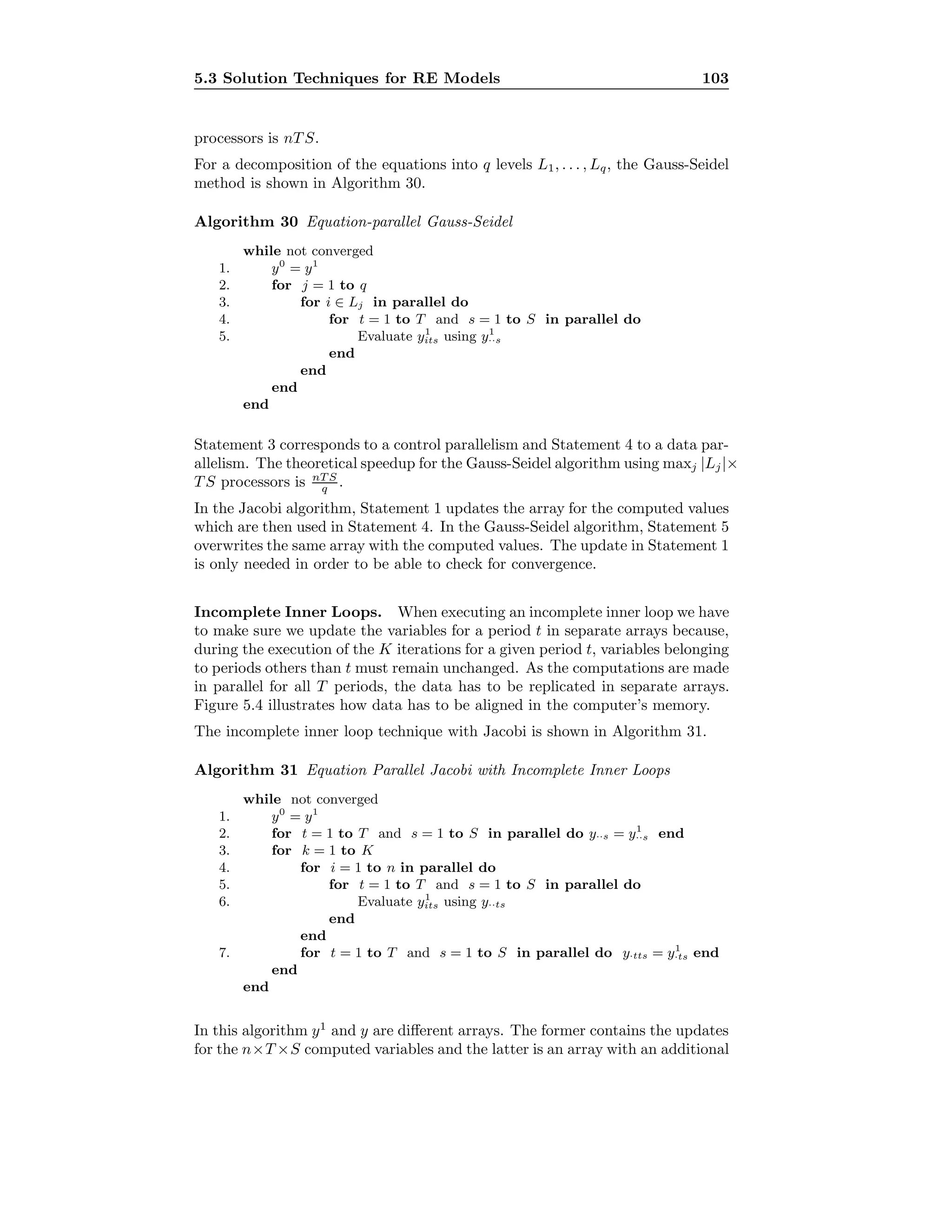

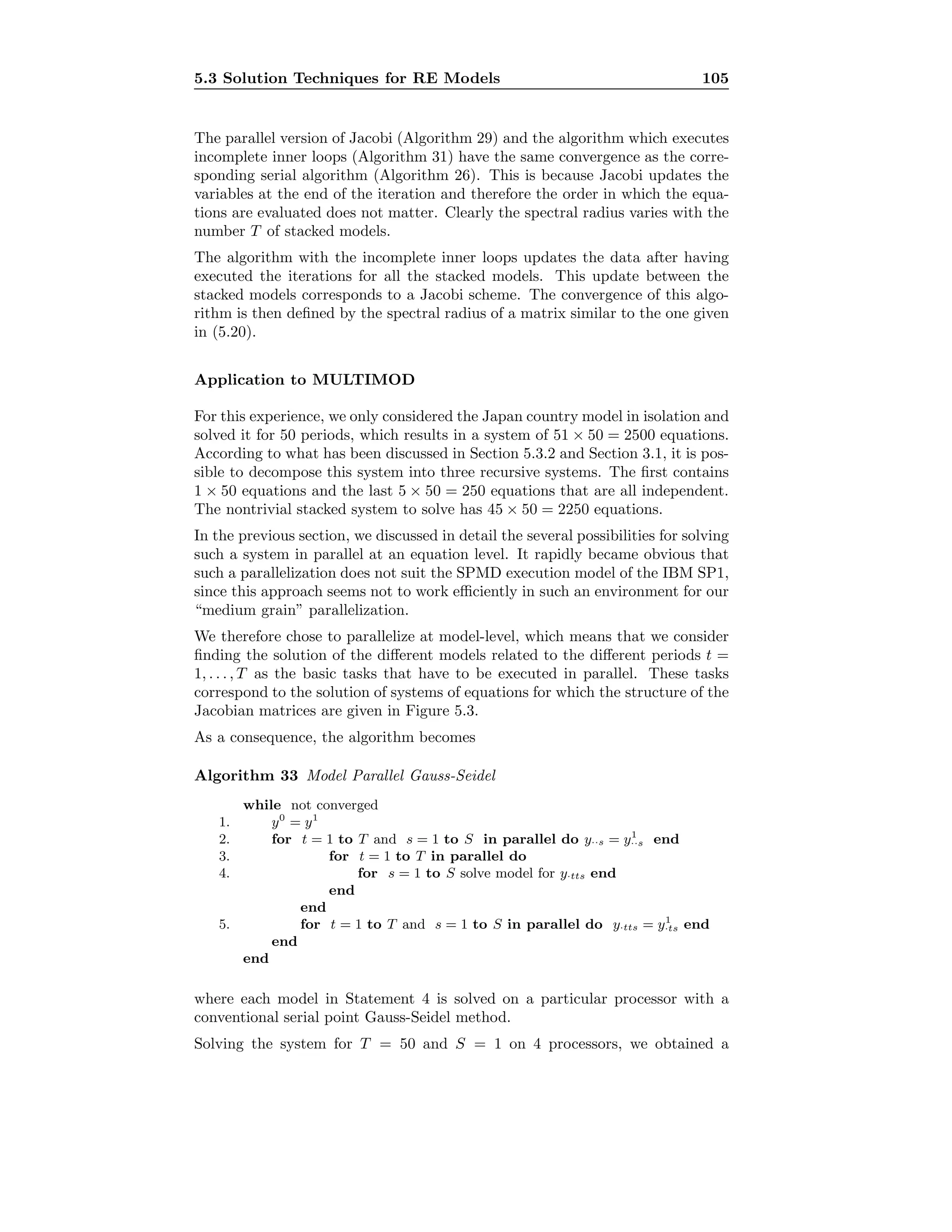
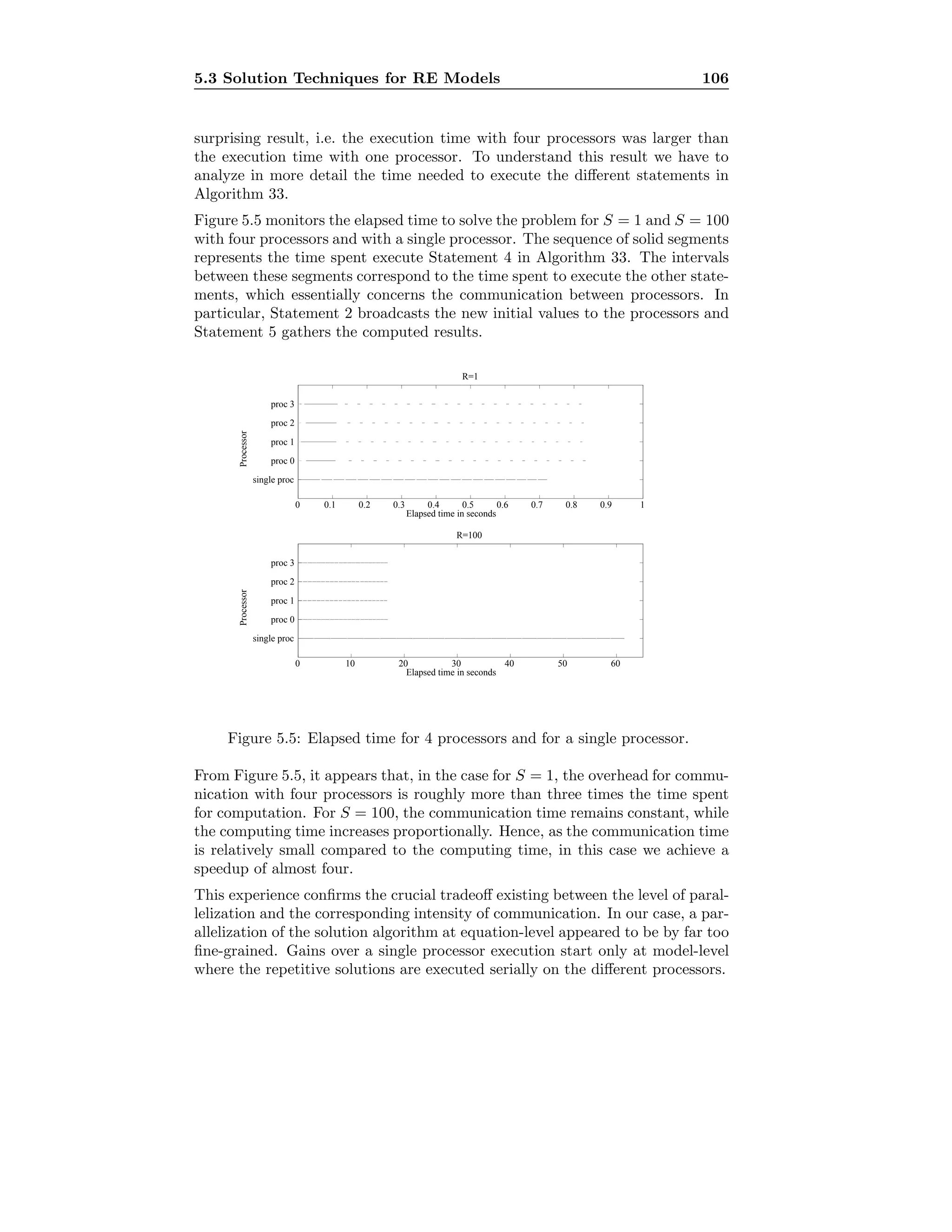
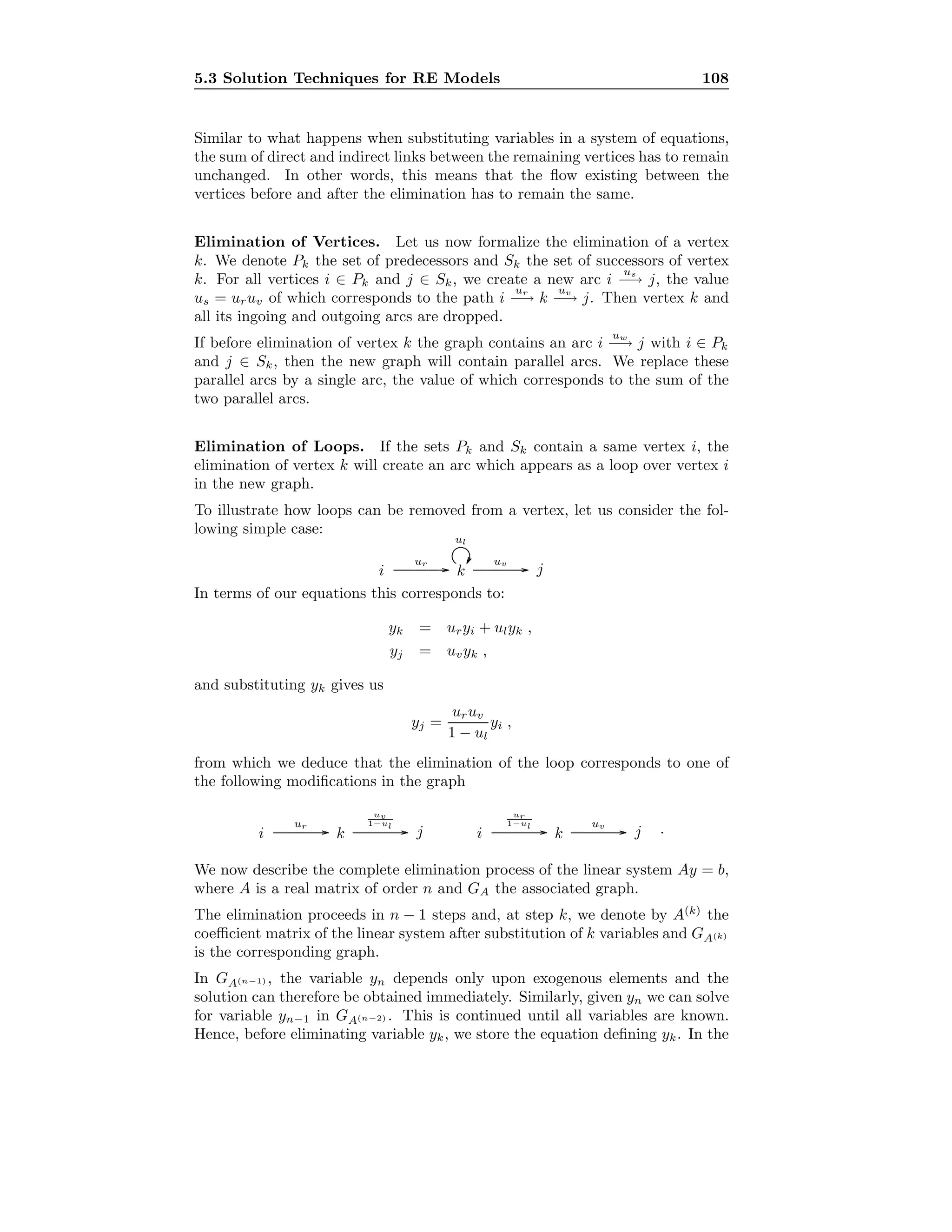
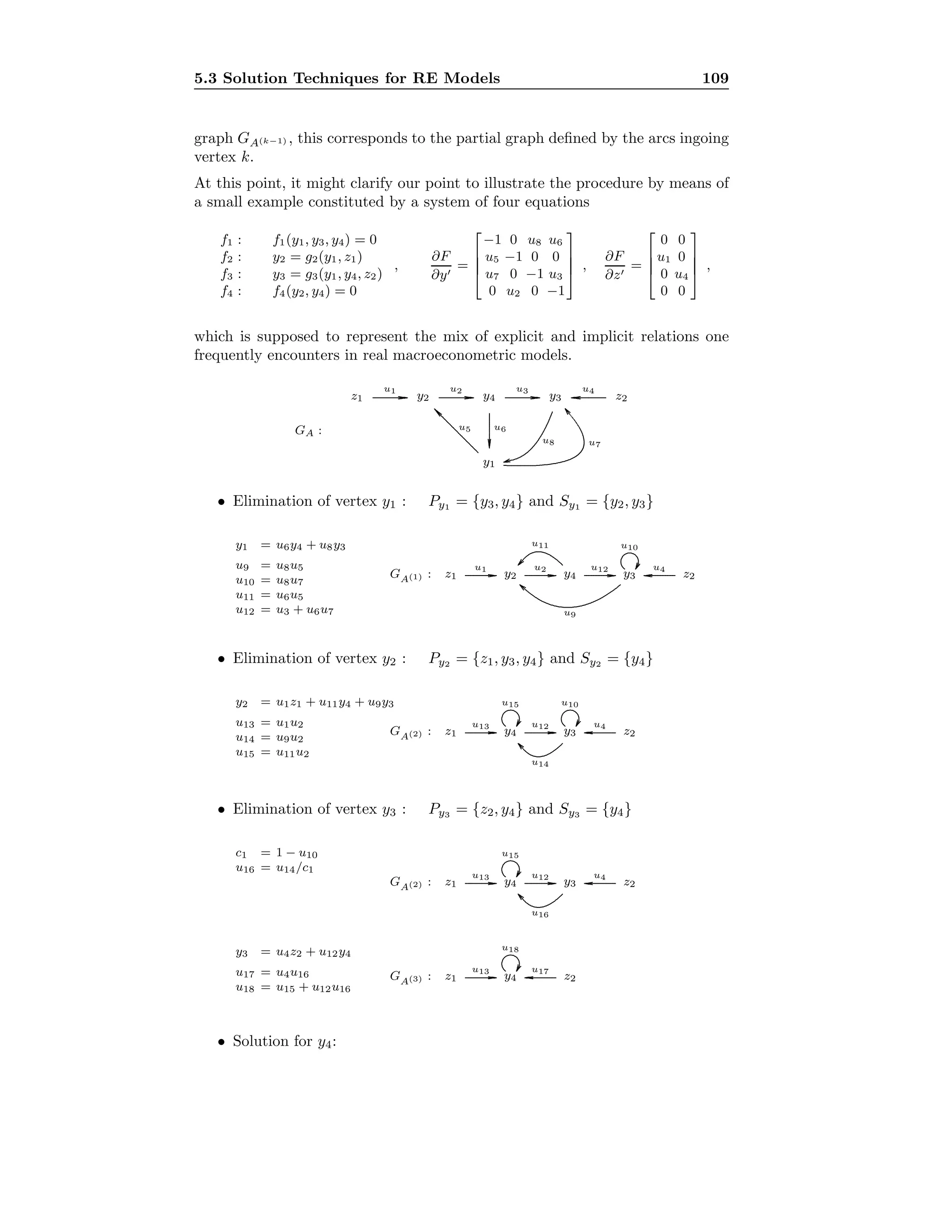
![5.3 Solution Techniques for RE Models 110
c2 = 1 − u18
y4 = (u13z1 + u17z2)/c2
Given the expressions for the forward substitutions and the backward substitu-
tions, the linear system of our example can be solved executing 29 elementary
arithmetic operations.
Minimizing the Fill-in. It is well known that, for a sparse Gaussian elimi-
nation, the choice of the variables to be substituted (pivots) is also conditioned
by making sure an excessive loss of sparsity is avoided.
From the illustration describing the procedure of vertex elimination, we see that
an upper bound for the number of new arcs generated is given by d−
k d+
k , the
product of indegree and outdegree of vertex k. We therefore select a vertex k
such that d−
k d+
k is minimum over all remaining vertices in the graph.2
We reconsider the previous example in order to illustrate the effect of the choice
of the order in which the variables are eliminated.
• Elimination of vertex y2 : Py2 = {z1, y1} and Sy2 = {y4}
y2 = u5y1 + u1z1
u9 = u1u2
u10 = u5u2
GA(1) :
y1
z1 y3y4 z2........................................................................
u9
........................................................................
u3
..............................................
.............
.............
u6
.............................................. ............. .............
u4
...................................................................................................................................................................................................................
u7
..................................................................................................................................
u8
................................................................................................................
...........
u10
• Elimination of vertex y3 : Py3 = {z2, y1, y4} and Sy3 = {y1}
y3 = u7y1 + u3y4 + u4z2
u11 = u4u8
u12 = u7u8
u13 = u3u8 + u6
GA(2) :
y1
z1 z2y4........................................................................
u9
..............................................
.............
.............
u13
..................................................................................................................................
u11
................................................................................................................
...........
u10
..........................................................................................
...........
u12
• Elimination of vertex y4 : Py4 = {z1, y1} and Sy4 = {y1}
y4 = u10y1 + u9z1
u14 = u9u13
u15 = u10u13 + u12
GA(3) :
y1
z1 z2
..................................................................................................................................
u11
........................................................................................................................ ...........
u14
..........................................................................................
...........
u15
• Solution for y1:
c1 = 1 − u15
y1 = (u14z1 + u11z2)/c1
2This is known as the Markowitz criterion, see Duff et al. [30, p. 128].](https://image.slidesharecdn.com/c12cdca8-ad4d-451a-b4fb-6c6bd72ac4d1-161015164104/75/t-118-2048.jpg)
![5.3 Solution Techniques for RE Models 111
For this order of vertices, the forward substitutions and the backward substitu-
tions necessitate only 24 elementary arithmetic operations.
Condition of the Linear System. In order to achieve a good numerical
solution for a linear system, two aspects are of crucial importance. The first is
the condition of the problem. If the problem is not reasonably well conditioned
there is little hope of obtaining a satisfactory solution. The second problem
concerns the method used which should be numerically stable. This means
roughly that the errors due to the floating point computations are not excessively
magnified. In the following, we will suggest practical guidelines which may prove
helpful to enhance the condition of a linear system.
Let us recall that the linear system we want to solve is given by J(k)
s = b.
We choose to associate a graph to this linear system. In order to do this, it
is necessary to select a normalization for the matrix J(
k). Such a normaliza-
tion corresponds to a particular row scaling of the original linear system. This
transformation modifies the condition of the linear system. Our goal is to find
a normalization for which the condition is likely to be good.
We recall that the condition κ of a matrix A in the frame of the solution of
linear system Ax = b is defined as
κp(A) = A p A−1
p ≥ 1 ,
and when κ(A) is large the matrix is said to be ill-conditioned. We know that
κp varies with the choice of the norm p, however this does not significantly affect
the order of magnitude of the condition number. In the following, p is assumed
∞ unless stated otherwise. Hence, we have
κ(A) = A A−1
,
with
A = max
i=1,...,n
n
j=1
|aij| .
Row scaling can significantly reduce the condition of a matrix. We therefore
look for a scaling matrix D for which
κ(D−1
A) κ(A) .
From a theoretical point of view, the problem of finding D minimizing κ(D−1
A)
has been solved for the infinity norm, see Bauer [10], however the result cannot
be used in practice. Our concern is to suggest a practical solution to this problem
by providing an efficient heuristic.
We certainly are aware that the problem of row scaling cannot be solved so far
automatically for any given matrix. A technique consists in choosing D such
that each row in D−1
A has approximately the same ∞-norm, see Golub and
Van Loan [56, p. 125].
As we want to represent our system using a graph for which we need a nor-
malization, the set of possible scaling matrices is finite. The idea about rows](https://image.slidesharecdn.com/c12cdca8-ad4d-451a-b4fb-6c6bd72ac4d1-161015164104/75/t-119-2048.jpg)
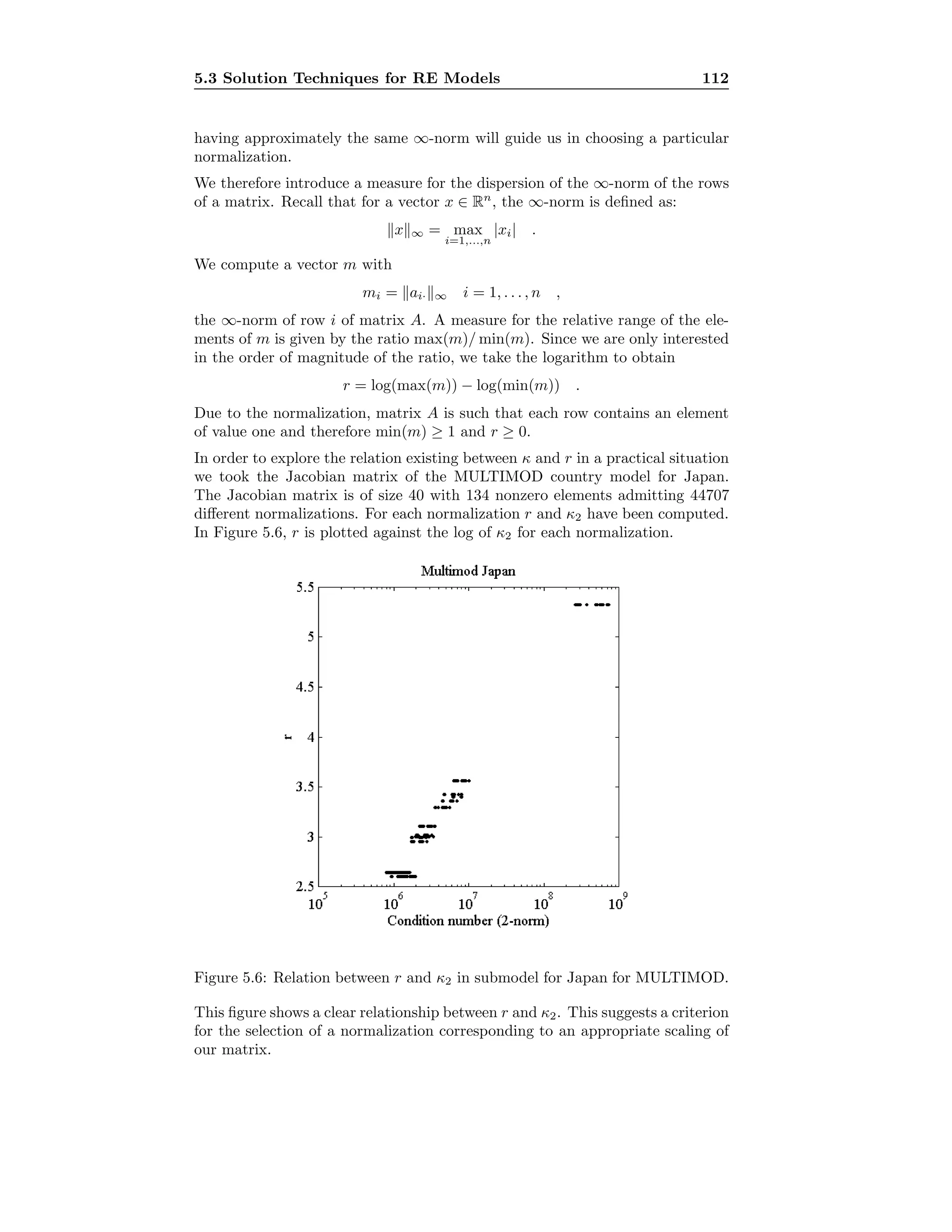
![5.3 Solution Techniques for RE Models 113
The selection of the normalization is then performed by seeking a matching in
a bipartite graph3
so that it optimizes a criterion built upon the values of the
edges, which in turn correspond to the entries of the Jacobian matrix of the
model.
Selection of Pivots. We know that the choice of the pivots in a Gaussian
elimination is determinant for the numerical stability. For the SGE method,
a partial pivoting strategy would require to resort once more to the bipartite
graph of the Jacobian matrix. In this case, for a given vertex, we choose new
adjacent matchings such that the edge belonging to the new matching is of
maximum magnitude.
A strategy for the achievement a reasonable fill-in is to apply a threshold such
as explained in Section 2.3.2. The Markowitz criterion is easy to implement in
order to select candidate vertices defining the edge in the new matching, since
this criterion only depends on the degree of the vertices.
Table 5.3 summarizes the operation counts for a Gauss-Seidel method and a
Newton method using two different sparse linear solvers. The Japan model is
solved for a single period and the counts correspond to the total number of
operations for the respective methods to converge. We recall that for the GS
method, we needed to find a new normalization and ordering of the equations,
which constitutes a difficult task. The two sparse Newton methods are similar
in their computational complexity: the advantage of the SGE method is that
this method reuses the symbolic factorizations of the Jacobian matrix between
successive iterations.
Newton
Statement MATLAB SGE GS
2 1.5 1.5 9.7
3 11.5 11.5 -
4 3.3 1.7 -
total 16.3 14.7 9.7
Table 5.3: Operation count in Mflops for Newton combined with SGE and
MATLAB’s sparse solver, and Gauss-Seidel.
The total count of operations clearly favors the sparse Newton method, as the
difficult task of appropriate renormalizing and reordering is not required then.
Multiple Blockdiagonal LU
Matrix S in 5.3.3 is a block partitioned matrix and the LU factorization of such
a matrix can be performed at block level. Such a factorization is called a block
LU factorization. To take advantage of the blockdiagonal structure of matrix S,
the block LU factorization can be adapted to a multiple blockdiagonal matrix
with r lower blocks and h upper blocks (see Golub and Van Loan [56, p. 171]).
3The association of a bipartite graph to the Jacobian matrix can be found in Gilli [50,
p. 100].](https://image.slidesharecdn.com/c12cdca8-ad4d-451a-b4fb-6c6bd72ac4d1-161015164104/75/t-121-2048.jpg)
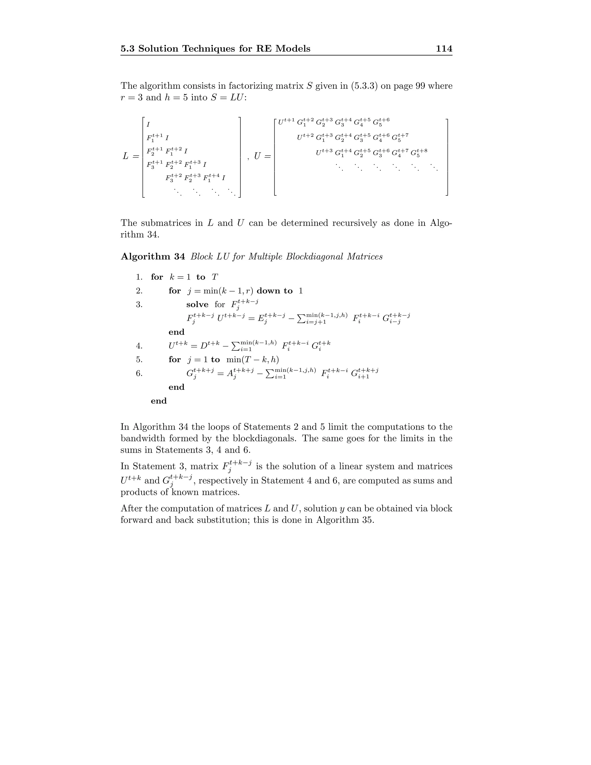
![5.3 Solution Techniques for RE Models 115
Algorithm 35 Block Forward and Back Substitution
1. ct+1
= bt+1
2. for k = 2 to T
3. ct+k
= bt+k
− min(k−1,r)
i=1 Ft+k−i
i ct+k−i
end
4. solve Ut+T
yt+T
= ct+T
for yt+T
5. for k = T − 1 down to 1
6. solve for yt+k
Ut+k
yt+k
= ct+k
− min(T −k,h)
i=1 Gt+k+i
i yt+k+i
end
Statements 1, 2 and 3 concern the forward substitution and Statements 4, 5
and 6 perform the back substitution. The F matrices in Statement 3 are al-
ready available after computation of the loop in Statement 2 of Algorithm 34.
Therefore the forward substitution could be done during the block LU factor-
ization.
From a numerical point of view, block LU does not guarantee the numerical
stability of the method even if Gaussian elimination with pivoting is used to
solve the subsystems. The safest method consists in solving the Newton step in
the stacked system with a sparse linear solver using pivoting. This procedure is
implemented in portable TROLL [67], which uses MA28, see Duff et al. [30].
Structure of the Submatrices in L and U. To a certain extent Block LU
already takes advantage of the sparsity of the system as the zero submatrices
are not considered in the computations. However, we want to go further and
exploit the invariance of the incidence matrices, i.e. their structure. As matrices
Et+k
i , Dt+k
and At+k
j have respectively the same sparse structure for all k, it
comes that the structure of matrices Ft+k
i , Ut+k
and Gt+k
j is also sparse and
predictable.
Indeed, if we execute the block LU Algorithm 34, we observe that the matrices
Ft+k
i , Ut+k
and Gt+k
j involve identical computations for min(r, h) k T −
min(r, h). These computations involve sparse matrices and may therefore be
expressed as sums of paths in the graphs corresponding to these matrices.
The computations involving structurally identical matrices can be performed
without repeating the steps used to analyze the structure of these matrices.
Parallelization. The block LU algorithm proceeds sequentially to compute
the different submatrices in L and U. The same goes for the block forward and
back substitution. In these procedures, the information necessary to execute a
given statement is always linked to the result of immediately preceeding state-
ments, which means that there are no immediate and obvious possibilities of
parallelizing the algorithm.
On the contrary, the matrix computations within a given statement offer ap-
pealing opportunities for parallel computations. If, for instance, one uses the](https://image.slidesharecdn.com/c12cdca8-ad4d-451a-b4fb-6c6bd72ac4d1-161015164104/75/t-123-2048.jpg)
![5.3 Solution Techniques for RE Models 116
SGE method suggested in Section 5.3.4 for the solution of the linear system,
the implementation of a data parallel execution model to perform efficiently
repeated independent solutions of the model turns out to be straightforward.
To identify task parallelism, we can analyze the structure of the operations
defined by the algebraic expressions discussed above. In order to do this, we seek
for sets of expressions which can be evaluated independently. We illustrate this
for the solution of the linear system presented on page 110. The identification
of the parallel tasks can be performed efficiently by resorting to a representation
of the expressions by means of a graph as shown in Figure 5.7.
u11 u10 u12 u13 u9
u15 u14
y1
y4 y2
y3
......................................................................................................................
.............
...............
......................
.............
..............
...................... ..............
.............
................................................................................ .................
...............
......................
.............
..............
...................... ..............
.............
.............
............
............
..................................................................................................................... .................
................
...................... ..............
.............
......................
.............
..............
.............
............
............
Figure 5.7: Scheduling of operations for the solution of the linear system as
computed on page 110.
We see that the solution can be computed in five steps, which each consist of
one to five parallel tasks.4
The elimination of a vertex yt
k (corresponding to variable yt
k) in the SGE al-
gorithm described in Section 5.3.4 allows interesting developments in a stacked
model. Let us consider a vertex yt
k for which there exists no vertex ys
j ∈ Pyt
k
∪Syt
k
for all j and s = t. In other words all the predecessors and successors of yt
k be-
long to the same period t. The operations for the elimination of such a vertex
are independent and identical for all the T variables yt
k, t = 1, . . . , T. Hence the
computation of the arcs defining the new graph resulting from the elimination
of such a vertex are executed only once and then evaluated (possibly in parallel)
for the different T periods. For the elimination of vertices yt
k with predecessors
and successors in period t + 1, it is again possible to split the model into in-
dependent pieces concerning periods [t, t + 1], [t + 2, t + 3] etc. for which the
elimination is again performed independently. This process can be continued
until elimination of all vertices.
Nonstationary Iterative Methods
This section reports results on numerical experiments with different nonstation-
ary iterative solvers that are applied to find the step in the Newton method.
We recall that the system is now stacked and has been decomposed into J∗
according to the decomposition technique explained earlier. The size of the
4This same approach has been applied for the parallel execution of Gauss-Seidel iterations
in Section 4.2.2.](https://image.slidesharecdn.com/c12cdca8-ad4d-451a-b4fb-6c6bd72ac4d1-161015164104/75/t-124-2048.jpg)
![5.3 Solution Techniques for RE Models 117
nontrivial system to be solved is T × 413, where T is the number of times the
model is stacked. Figure 5.8 shows the pattern of the stacked model for T = 10.
Figure 5.8: Incidence matrix of the stacked system for T = 10.
The nonstationary solvers suited for nonsymmetric problems suggested in the
literature we chose to experiment are BiCGSTAB, QMR and GMRES(m). The
QMR method (Quasi-Minimal Residual) introduced by Freund and Nachti-
gal [40] has not been presented in Section 2.5 since the method presents poten-
tials for failures if implemented without sophisticated look-ahead procedures.
We tried a version of QMR without look-ahead strategies for our application.
BiCGSTAB—proposed by van der Vorst [99]—is also designed to solve large
and sparse nonsymmetric linear systems and usually displays robust features
and small computational cost. Finally, we chose to experiment the behavior in
our framework of GMRES(m) originally presented by Saad and Schultz [90].
For all these methods, it is known that preconditioning can greatly influence
the convergence. Therefore, following some authors (e.g. Concus et al. [24],
Axelsson [6] and Bruaset [21]), we applied a preconditioner based upon the
block structure of our problem.
The block preconditioner we used is built on the LU factorization of the first
block of our stacked system. If we dropped the leads and lags of the model, the
Jacobian matrix would be block diagonal, i.e.
Dt+1
Dt+2
...
Dt+T
.
The tradeoff between the cost of applying the preconditioner and the expected
gain in convergence speed can be improved by using a same matrix D along](https://image.slidesharecdn.com/c12cdca8-ad4d-451a-b4fb-6c6bd72ac4d1-161015164104/75/t-125-2048.jpg)
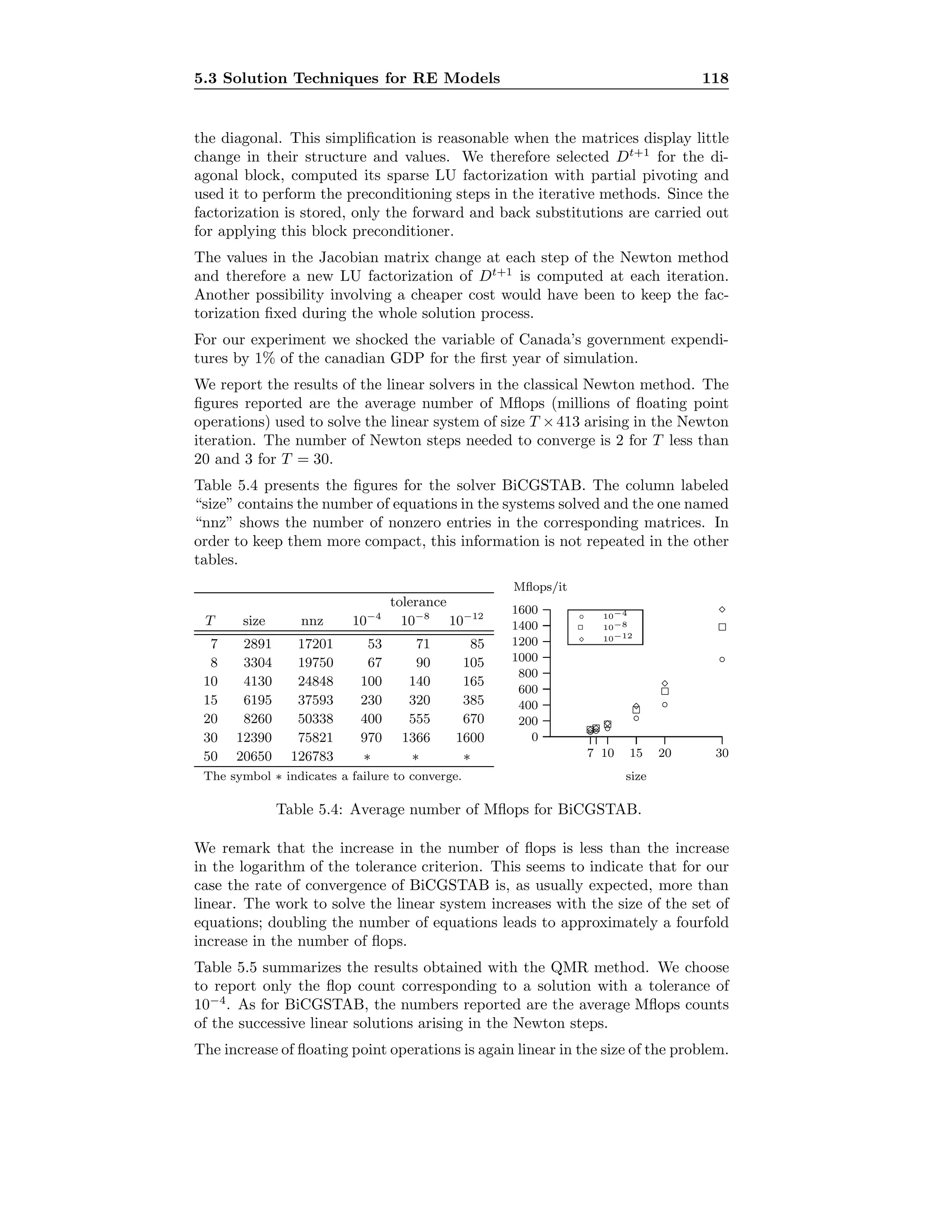
![5.3 Solution Techniques for RE Models 119
T tol=10−4
7 91
8 120
10 190
15 460
20 855
30 2100
50 9900∗
∗Average of the first two
Newton steps; failure to con-
verge in the third step. 7 10 15 20 30
size
0
200
400
600
800
1000
1200
1400
1600
1800
2000
◦◦ ◦
◦
◦
◦
Mflops/it
Table 5.5: Average number of Mflops for QMR.
The QMR method seems however, about twice as expensive as BiCGSTAB
for the same tolerance level. The computational burden of QMR consists of
about 14 level-1 BLAS and 4 level-2 BLAS operations, whereas BiCGSTAB
uses 10 level-1 BLAS and 4 level-2 BLAS operations. This apparently indicates
a better convergence behavior of BiCGSTAB than of QMR.
Table 5.6 presents a summary of the results obtained with the GMRES(m)
technique.
Like in the previous methods, the convergence displays the expected superlinear
convergence behavior. Another interesting feature of GMRES(m) is the possibil-
ity of tuning the restart parameter m. We know that the storage requirements
increase with m and that the larger m becomes, the more likely the method
converges, see [90, p. 867]. Each iteration uses approximately 2m + 2 level-1
BLAS and 2 level-2 BLAS operations.
To confirm the fact that the convergence will take place for sufficiently large m,
we ran a simulation of our model with T = 50, tol=10−4
and m = 50. In this
case, the solver converged with an average count of 9900 Mflops.
It is also interesting to notice that long restarts, i.e. large values of m, do
not in general generate much heavier computations and that the increase in
convergence may even lead to diminishing the global computational cost. An
operation count per iteration is given in [90], which clearly shows this feature
of GMRES(m).
Even though this last method is not cheaper than BiCGSTAB in terms of flops,
the possibility of overcoming nonconvergent cases by using larger values of m
certainly favors GMRES(m).
Finally, we used the sparse LU solver provided in MATLAB. For general non-
symmetric matrices, a strategy that this method implements is to reorder the
columns according to their minimum degree in order to minimize the fill-in.
On the other hand, a sparse partial pivoting technique proposed by Gilbet and
Peierls [45] is used to prevent losses in the stability of the method. In Table 5.7,
we present some results obtained with the method we have just described.](https://image.slidesharecdn.com/c12cdca8-ad4d-451a-b4fb-6c6bd72ac4d1-161015164104/75/t-127-2048.jpg)
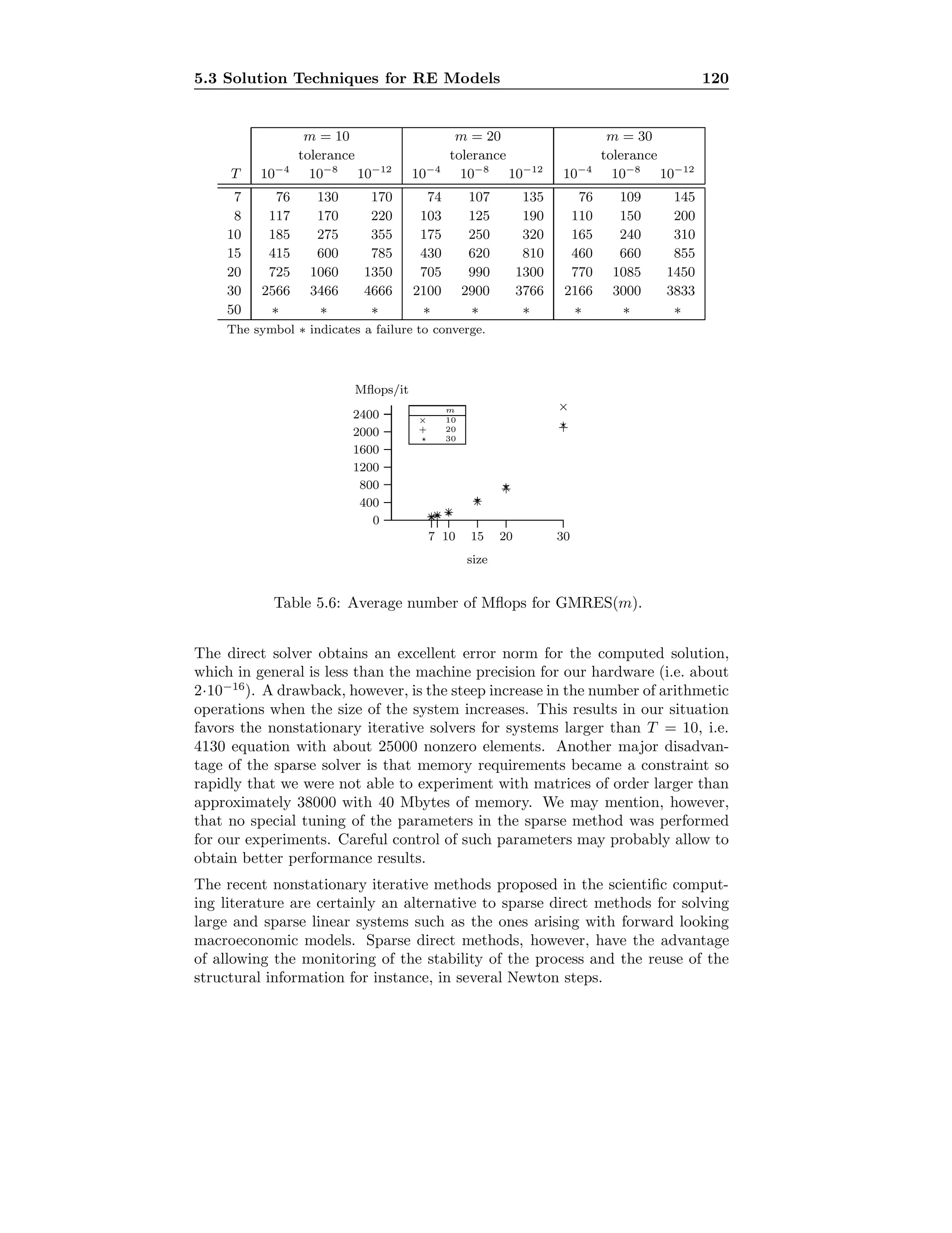
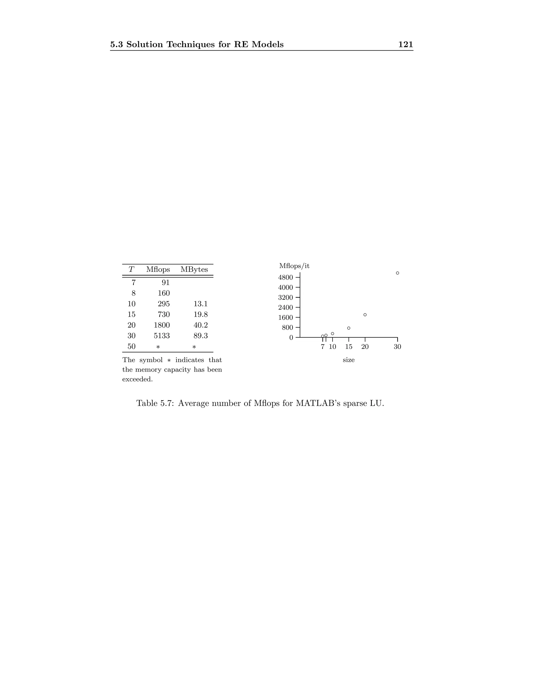
![Appendix A
The following pages provide background material on computation in finite pre-
cision and an introduction to computational complexity—two issues directly
relevant to the discussions of numerical algorithms.
A.1 Finite Precision Arithmetic
The representation of numbers on a digital computer is very different from the
one we usually deal with. Modern computer hardware, can only represent a
finite subset of the real numbers. Therefore, when a real number is entered
in a computer, a representation error generally appears. The effects of finite
precision arithmetic are thoroughly discussed in Forsythe et al. [38] and Gill et
al. [47] among others.
We may explain what occurs by first stating that the internal representation of
a real number is a floating point number. This representation is characterized
by the number base β, the precision t and the exponent range [L, U], all four
being integers.
The form of the set of all floating point numbers F is
F = {f | f = ±.d1d2 . . . dt × βe
and 0 ≤ di β, i = 1, . . . , n, d1 = 0, L e U}
∪ {0} .
Nowadays, the standard base is β = 2, whereas the other integers t, L, U vary
according to the hardware; the number .d1d2 . . . dt is called the mantissa. The
magnitudes of the largest and smallest representable numbers are
M = βU
(1 − β−t
) for the largest,
m = βL−1
for the smallest.
Therefore, when we input x ∈ R in a computer it is replaced by fl(x) which is the
closest number to x in F. The term “closest” is defined as the nearest number
in F (rounded away from zero if there is a tie) when rounded arithmetic is used
and the nearest number in F such as |fl(x)| ≤ |x| when chopped arithmetic is
used.](https://image.slidesharecdn.com/c12cdca8-ad4d-451a-b4fb-6c6bd72ac4d1-161015164104/75/t-130-2048.jpg)


![A.3 Complexity of Algorithms 125
We note that κ(A) depends on the norm used. With this interpretation, it is
clear that κ(A) must be greater than or equal to 1 and the closer to singularity
matrix A is, the greater κ(A) becomes. In the limiting case where A is singular,
the minimum stretch is zero and the condition number is defined to be infinite.
It is certainly not operational to compute the condition number of A by the
formula A−1
A . This number can be estimated by other procedures when
the 1 norm is used. A classical reference is Cline et al. [23] and the LAPACK
library.
A.3 Complexity of Algorithms
The analysis of the computational complexity of algorithms is a very sophis-
ticated and difficult topic in computer science. Our goal is simply to present
some terminology and distinctions that are of interest in our work.
The solution of most problems can be approached using different algorithms.
Therefore, it is natural to try to compare their performance in order to find
the most efficient method. In its broad sense, the efficiency of an algorithm
takes into account all the computing resources needed for carrying out its ex-
ecution. Usually, for our purposes, the crucial resource will be the computing
time. However, there are other aspects of importance such as the amount of
memory needed (space complexity) and the reliability of an algorithm. Some-
times a simpler implementation can be preferred to a more sophisticated one,
for which it becomes difficult to assess the correctness of the code.
Keeping these caveats in mind, it is nonetheless very informative to calculate
the time requirement of an algorithm. The techniques presented in the following
deal with numerical algorithms, i.e. algorithms were the largest part of the time
is devoted to arithmetic operations. With serial computers, there is an almost
proportional relationship between the number of floating point operations (ad-
ditions, subtractions, multiplications and divisions) and the running time of an
algorithm. Clearly, this time is very specific to the computer used, thus the
quantity of interest is the number of flops (floating point operations) used.
The time requirements of an algorithm are conveniently expressed in terms of the
size of the problem. In a broad sense, this size usually represents the number of
items describing the problem or a quantity that reflects it. For a general square
matrix A with n rows and n columns, a natural size would be its order n.
We will focus on the time complexity function which expresses, for a given
algorithm, the largest amount of time needed to solve a problem as a function
of its size. We are interested in the leading terms of the complexity function so
it is useful to define a notation.
Definition 3 Let f and g be two functions f, g : D → R, D ⊆ R.
1. f(x) = O(g(x)) if and only if there exists a constant a 0 and xa such
that for every x ≥ xa we have |f(x)| ≤ a g(x),
2. f(x) = Ω(g(x)) if and only if there exists a constant b 0 and xb such
that for every x ≥ xb we have f(x) ≥ b g(x),](https://image.slidesharecdn.com/c12cdca8-ad4d-451a-b4fb-6c6bd72ac4d1-161015164104/75/t-133-2048.jpg)
![A.3 Complexity of Algorithms 127
An important distinction is made between polynomial time algorithms, the time
complexity of which is O(p(n)), where p(n) is some polynomial function in n,
and non deterministic polynomial time algorithms. The class of polynomial is
denoted by P; nonpolynomial time algorithms fall in the class NP. For an exact
definition and clear exposition about P and NP classes see Even [32] and Garey
and Johnson [43]. Clearly, we cannot expect nonpolynomial algorithms to solve
problems efficiently. However they sometimes are applicable for some small val-
ues of n. In very few cases, as the bound found is a worst-case complexity, some
nonpolynomial algorithms behave quite well in an average case complexity anal-
ysis (as, for instance, the simplex method or the branch-and-bound method).](https://image.slidesharecdn.com/c12cdca8-ad4d-451a-b4fb-6c6bd72ac4d1-161015164104/75/t-135-2048.jpg)
![Bibliography
[1] L. Adams. M-Step Preconditioned Conjugate Gradient Methods. SIAM J. Sci.
Stat. Comput., 6:452–463, 1985.
[2] A. V. Aho, J. E. Hopcroft, and J. D. Ullman. The Design and Analysis of
Computer Algorithms. Addison-Wesley, Reading, MA, 1974.
[3] H. M. Amman. Nonlinear Control Simulation on a Vector Machine. Parallel
Computing, 10:123–127, 1989.
[4] A. Ando, P. Beaumont, and M. Ando. Efficiency of the CYBER 205 for Stochas-
tic Simulation of A Simultaneous, Nonlinear, Dynamic Econometric Model. Iter-
nat. J. Supercomput. Appl., 1(4):54–81, 1987.
[5] J. Armstrong, R. Black, D. Laxton, and D. Rose. A Robust Method for Simulat-
ing Forward-Looking Models. The Bank of Canada’s New Quarterly Projection
Model, Part 2. Technical Report 73, Bank of Canada, Ottawa, Canada, 1995.
[6] O. Axelsson. Incomplete Block Matrix Factorization Preconditioning Methods.
The Ultimate Answer? J. Comput. Appl. Math., 12:3–18, 1985.
[7] O. Axelsson. Iterative Solution Methods. Oxford University Press, Oxford, UK,
1994.
[8] R. Barrett et al. Templates for the Solution of Linear Systems: Building Blocks
for Iterative Methods. SIAM, Philadelphia, PA, 1994.
[9] R. J. Barro. Rational Expectations and the Role of Monetary Policy. Journal
of Monetary Economics, 2:1–32, 1976.
[10] F. L. Bauer. Optimally Scaled Matrices. Numer. Math., 5:73–87, 1963.
[11] R. Becker and B. Rustem. Algorithms for Solving Nonlinear Models. PROPE
Discussion Paper 119, Imperial College, London, 1991.
[12] M. Beenstock. A Neoclassical Analysis of Macroeconomic Policy. Cambridge
University Press, London, 1980.
[13] M. Beenstock, A. Dalziel, P. Lewington, and P. Warburton. A Macroeconomic
Model of Aggregate Supply and Demand for the UK. Economic Modelling,
3:242–268, 1986.
[14] K. V. Bhat and B. Kinariwala. Optimum Tearing in Large Systems and
Minimum Feedback Cutsets of a Digraph. Journal of the Franklin Institute,
307(2):71–154, 1979.
[15] C. Bianchi, G. Bruno, and A. Cividini. Analysis of Large Scale Econometric
Models Using Supercomputer Techniques. Comput. Sci. Econ. Management,
5:271–281, 1992.
[16] L. Bodin. Recursive Fix-Point Estimation, Theory and Applications. Selected
Publications of the Department of Statistics. University of Uppsala, Uppsala,
Norway, 1974.](https://image.slidesharecdn.com/c12cdca8-ad4d-451a-b4fb-6c6bd72ac4d1-161015164104/75/t-136-2048.jpg)
![BIBLIOGRAPHY 129
[17] R. Boucekkine. An Alternative Methodology for Solving Nonlinear Forward-
looking Models. Journal of Economic Dynamics and Control, 19:711–734, 1995.
[18] A. S. Brandsma. The Quest Model of the European Community. In S. Ichimura,
editor, Econometric Models of Asian-Pacific Countries. Springer-Verlag, Tokyo,
1994.
[19] F. Brayton and E. Mauskopf. The Federal Reserve Board MPS Quarterly Econo-
metric Model of the U.S. Economy. Econom. Modelling, 2(3):170–292, 1985.
[20] C. J. Broyden. A Class of Methods for Solving Nonlinear Simultaneous Equa-
tions. Mathematics of Computation, 19:577–593, 1965.
[21] A. M. Bruaset. Efficient Solutions of Linear Equations Arising in a Nonlinear
Economic Model. In M. Gilli, editor, Computational Economics: Models, Meth-
ods and Econometrics, Advances in Computational Economics. Kluwer Aca-
demic Press, Boston, MA, 1995.
[22] L. K. Cheung and E. S. Kuh. The Bordered Triangular Matrix and Miminum
Essential Sets of a Digraph. IEEE Transactions on Circuits and Systems,
21(1):633–639, 1974.
[23] A. K. Cline, C. B. Moler, G. W. Stewart, and J. H. Wilkinson. An Estimate for
the Condition Number of a Matrix. SIAM J. Numer. Anal., 16:368–375, 1979.
[24] P. Concus, G. Golub, and G. Meurant. Block Preconditioning for the Conjugate
Gradient Method. SIAM J. Sci. Stat. Comput., 6:220–252, 1985.
[25] J. E. Jr. Dennis and J. J. Mor´e. A Characterization of Superlinear Convergence
and its Application to Quasi-Newton Methods. Mathematics of Computation,
28:549–560, 1974.
[26] J. E. Jr. Dennis and R. B. Schnabel. Numerical Methods for Unconstrained
Optimization and Nonlinear Equations. Series in Computational Mathematics.
Prentice-Hall, Englewood Cliffs, NJ, 1983.
[27] H. Don and G. M. Gallo. Solving Large Sparse Systems of Equation in Econo-
metric Models. Journal of Forecasting, 6:167–180, 1987.
[28] P. Dubois, A. Greenbaum, and G. Rodrigue. Approximating the Inverse of
a Matrix for Use in Iterative Algorithms on Vector Processors. Computing,
22:257–268, 1979.
[29] I. S. Duff. MA28 – A Set of FORTRAN Subroutines for Sparse Unsymmetric
Linear Equations. Technical Report AERE R8730, HMSO, London, 1977.
[30] I. S. Duff, A. M. Erisman, and J. K. Reid. Direct Methods for Sparse Matrices.
Oxford Science Publications, New York, 1986.
[31] I. S. Duff and J. K. Reid. The Design of MA48, a Code for the Direct Solution of
Sparse Unsymmetric Linear Systems of Equations. Technical Report RAL-TR-
95-039, Computer and Information Systems Department, Rutherford Appelton
Laborartory, Oxfordshire, August 1995.
[32] S. Even. Graph Algorithms. Computer Sience Press, Rockville, MD, 1979.
[33] R. C. Fair. Specification, Estimation and Analysis of Macroeconometric Models.
Harvard University Press, Cambridge, MA, 1984.
[34] R. C. Fair and J. B. Taylor. Solution and Maximum Likelihood Estimation of
Dynamic Nonlinear Rational Expectations Models. Econometrica, 51(4):1169–
1185, 1983.
[35] J. Faust and R. Tryon. A Distributed Block Approach to Solving Near-Block-
Diagonal Systems with an Application to a Large Macroeconometric Model. In
M. Gilli, editor, Computational Economics: Models, Methods and Econometrics,
Advances in Computational Economics. Kluwer Academic Press, Boston, MA,
1995.](https://image.slidesharecdn.com/c12cdca8-ad4d-451a-b4fb-6c6bd72ac4d1-161015164104/75/t-137-2048.jpg)
![BIBLIOGRAPHY 130
[36] P. Fisher. Rational Expectations in Macroeconomic Models. Kluwer Academic
Publishers, Dordrecht, 1992.
[37] P. G. Fisher and A. J. Hughes-Hallett. An Efficient Solution Strategy for Solv-
ing Dynamic Nonlinear Rational Expectations Models. Journal of Economic
Dynamics and Control, 12:635–657, 1988.
[38] G. E. Forsythe, M. A. Malcolm, and C. B. Moler. Computer Methods for Math-
ematical Computations. Prentice-Hall, Englewood Cliffs, NJ, 1977.
[39] R. W. Freund, G. H. Golub, and N. M. Nachtigal. Iterative Solution of Linear
Systems. Acta Numerica, pages 1–44, 1991.
[40] R. W. Freund and N. M. Nachtigal. QMR: A Quasi-mininal Residual Method
for Non-Hermitian Linear Systems. Numer. Math., 60:315–339, 1991.
[41] J. Gagnon. A Forward-Looking Multicountry Model for Policy Analysis: MX3.
Jornal of Economic and Financial Computing, 1:331–361, 1991.
[42] M. Garbely and M. Gilli. Two Approaches in Reading Model Interdependencies.
In J.-P. Ancot, editor, Analysing the Structure of Econometric Models, pages 15–
33. Martinus Nijhoff, The Hague, 1984.
[43] M. R. Garey and D. S. Johnson. Computers and Intractability, A Guide to the
Theory of NP-Completeness. W.H. Freeman and Co., San Francisco, 1979.
[44] J. R. Gilbert, C. B. Moler, and R. Schreiber. Sparse Matrices in MATLAB:
Design and Implementation. SIAM J. Matrix Anal. Appl., 13:333–356, 1992.
[45] J. R. Gilbert and Peierls. Sparse Partial Pivoting in Time Proportional to
Arithmetic Operations. SIAM J. Sci. Statist. Comput., 9:862–874, 1988.
[46] P. E. Gill, W. Murray, and M. H. Wright. Practical Optimization. Academic
Press, London, 1981.
[47] P. E. Gill, W. Murray, and M. H. Wright. Numerical Linear Algebra and Opti-
mization. Advanced Book Program. Addison-Wesley, Redwood City, CA, 1991.
[48] M. Gilli. CAUSOR — A Program for the Analysis of Recursive and Interdepen-
dent Causal Structures. Technical Report 84.03, Departement of Econometrics,
University of Geneva, 1984.
[49] M. Gilli. Causal Ordering and Beyond. International Economic Review,
33(4):957–971, 1992.
[50] M. Gilli. Graph-Theory Based Tools in the Practice of Macroeconometric Mod-
eling. In S. K. Kuipers, L. Schoonbeek, and E. Sterken, editors, Methods and
Applications of Economic Dynamics, Contributions to Economic Analysis. North
Holland, Amsterdam, 1995.
[51] M. Gilli and M. Garbely. Matching, Covers, and Jacobian Matrices. Journal of
Economic Dynamics and Control, 20:1541–1556, 1996.
[52] M. Gilli, M. Garbely, and G. Pauletto. Equation Reordering for Iterative Pro-
cesses — A Comment. Computer Science in Economics and Management, 5:147–
153, 1992.
[53] M. Gilli and G. Pauletto. Econometric Model Simulation on Parallel Computers.
International Journal of Supercomputer Applications, 7:254–264, 1993.
[54] M. Gilli and E. Rossier. Understanding Complex Systems. Automatica,
17(4):647–652, 1981.
[55] G. H. Golub and J. M. Ortega. Scientific Computing: An Introduction with
Parallel Computing. Academic Press, San Diego, CA, 1993.
[56] G. H. Golub and C. F. Van Loan. Matrix Computations. Johns Hopkins, Balti-
more, 1989.](https://image.slidesharecdn.com/c12cdca8-ad4d-451a-b4fb-6c6bd72ac4d1-161015164104/75/t-138-2048.jpg)
![BIBLIOGRAPHY 131
[57] G. Guardabassi. A Note on Minimal Essential Sets. IEEE Transactions on
Circuit Theory, 18:557–560, 1971.
[58] G. Guardabassi. An Indirect Method for Minimal Essential Sets. IEEE Trans-
actions on Circuits and Systems, 21(1):14–17, 1974.
[59] A. Hadjidimos. Accelerated Overrelaxation Method. Mathematics of Computa-
tion, 32:149–157, 1978.
[60] L. A. Hageman and D. M. Young. Applied Iterative Methods. Computer Science
and Applied Mathematics. Academic Press, Orlando, FL, 1981.
[61] S. G. Hall. On the Solution of Large Economic Models with Consistent Expec-
tations. Bulletin of Economic Research, 37:157–161, 1985.
[62] L. P. Hansen and T. J. Sargent. Formulating and Estimating Dynamic Linear
Rational Expectations Models. Journal of Economic Dynamics and Control,
2:7–46, 1980.
[63] J. Helliwell et al. The Structure of RDX2—Part 1 and 2. Staff Research Studies 7,
Bank of Canada, Ottawa, Canada, 1971.
[64] M. R. Hestenes and E. Stiefel. Method of Conjugate Gradients for Solving Linear
Systems. J. Res. Nat. Bur. Stand., 49:409–436, 1952.
[65] F. J. Hickernell and K. T. Fang. Combining Quasirandom Search and Newton-
Like Methods for Nonlinear Equations. Technical Report MATH–037, Departe-
ment of Mathematics, Hong Kong Baptist College, 1993.
[66] High Performance Fortran Forum, Houston, TX. High Performance Fortran
Language Specification. Version 0.4, 1992.
[67] P. Hollinger and L. Spivakovsky. Portable TROLL 0.95. Intex Solution, Inc., 35
Highland Circle, Needham, MA 02194, Preliminary Draft edition, May 1995.
[68] A. J. Hughes Hallett. Multiparameter Extrapolation and Deflation Methods for
Solving Equation Systems. International Journal of Mathematics and Mathe-
matical Sciences, 7:793–802, 1984.
[69] A. J. Hughes Hallett. Techniques Which Accelerate the Convergence of First
Order Iterations Automatically. Linear Algebra and Applications, 68:115–130,
1985.
[70] A. J. Hughes Hallett. A Note on the Difficulty of Comparing Iterative Processes
with Differing Rates of Convergence. Comput. Sci. Econ. Management, 3:273–
279, 1990.
[71] A. J. Hughes Hallett, Y. Ma, and Y. P. Ying. Hybrid Algorithms with Auto-
matic Switching for Solving Nonlinear Equations Systems in Economics. Com-
putational Economics, forthcoming 1995.
[72] R. M. Karp. Reducibility Among Combinatorial Problems. In R. E. Miller and
J. W. Thatcher, editors, Complexity of Computer Computations, pages 85–104.
Plenum Press, New York, 1972.
[73] C. T. Kelley. Iterative Methods for Linear and Nonlinear Systems of Equations.
Frontiers in Applied Mathematics. SIAM, Phildelphia, PA, 1995.
[74] J.-P. Laffargue. R´esolution d’un mod`ele macro´econom´etrique avec anticipations
rationnelles. Annales d’Economie et Statistique, 17:97–119, 1990.
[75] R. E. Lucas and T. J. Sargent, editors. Rational Expectations and Econometric
Practice. George Allen Unwin, London, 1981.
[76] R. E. Lucas, Jr. Some International Evidence on Output-Inflation Tradeoffs.
American Economic Review, 63:326–334, 1973.](https://image.slidesharecdn.com/c12cdca8-ad4d-451a-b4fb-6c6bd72ac4d1-161015164104/75/t-139-2048.jpg)
![BIBLIOGRAPHY 132
[77] R. E. Lucas, Jr. Econometric Policy Evaluation: A Critique. In K. Brunner
and A. H. Meltzer, editors, The Phillps Curve and Labor Markets, volume 1 of
Supplementary Series to the Jornal of Monetary Economics, pages 19–46. North
Holland, 1976.
[78] D. G. Luenberger. Linear and Nonlinear Programming. Addison-Wesley, Read-
ing, MA, second edition, 1989.
[79] P. Masson, S. Symanski, and G. Meredith. MULTIMOD Mark II: A Revised and
Extended Model. Occasional Paper 71, International Monetary Fund, Washing-
ton D.C., July 1990.
[80] B. T. McCallum. Rational Expectations and the Estimation of Econometric
Models: An Alternative Procedure. International Economic Review, 17:484–
490, 1976.
[81] A. Nagurney. Parallel Computation. In H. M. Amman, D. Kendrick, and J. Rust,
editors, Handbook of Computational Economics. North Holland, Amsterdam,
forthcoming 1995.
[82] P. Nepomiastchy and A. Ravelli. Adapted Methods for Solving and Optimizing
Quasi-Triangular Econometric Models. Anals of Economics and Social Measure-
ment, 6:555–562, 1978.
[83] P. Nepomiastchy, A. Ravelli, and F. Rechenmann. An Automatic Method to
Get an Econometric Model in Quasi-triangular Form. Technical Report 313,
INRIA, 1978.
[84] T. Nijman and F. Palm. Generalized Least Square Estimation of Linear Mod-
els Containing Rational Future Expectations. International Economic Review,
32:383–389, 1991.
[85] J. M. Ortega and W. C. Rheinboldt. Iterative Solution of Nonlinear Equations
in Several Variables. Academic Press, New York, 1970.
[86] L. Paige and M. Saunders. Solution of Sparse Indefinite Systems of Linear
Equations. SIAM J. Numer. Anal., 12:617–629, 1975.
[87] C. E. Petersen and A. Cividini. Vectorization and Econometric Model Simula-
tion. Comput. Sci. Econ. Management, 2:103–117, 1989.
[88] A. Pothen and C. Fan. Computing the Block Triangular Form of a Sparse
Matrix. ACM Trans. Math. Softw., 16(4):303–324, 1990.
[89] J. K. Reid, editor. Large Sparse Sets of Linear Equations. Academic Press,
London, 1971.
[90] Y. Saad and M. Schultz. GMRES: A Generalized Minimal Residual Algorithm
for Solving Nonsymmetric Linear Systems. SIAM J. Sci. Stat. Comput., 7:856–
869, 1986.
[91] T. J. Sargent. Rational Expectations, the Real Rate of Interest, and the Natural
Rate of Unemployment. Brooking Papers on Economic Activity, 2:429–480, 1973.
[92] T. J. Sargent. A Classical Macroeconometric Model for the United States. Jour-
nal of Political Economy, 84(2):207–237, 1976.
[93] R. Sedgewick. Algorithms. Addison Wesley, Reading, MA, 2nd edition, 1983.
[94] D. Steward. Partitioning and Tearing Systems of Equations. SIAM J. Numer.
Anal., 7:856–869, 1965.
[95] J. C. Strikwerda and S. C. Stodder. Convergence Results for GMRES(m). De-
partment of Computer Sciences, University of Wisconsin, August 1995.
[96] J. B. Taylor. Estimation and Control of a Macroeconometric Model with Ratio-
nal Expectations. Econometrica, 47(5):1267–1286, 1979.](https://image.slidesharecdn.com/c12cdca8-ad4d-451a-b4fb-6c6bd72ac4d1-161015164104/75/t-140-2048.jpg)
![BIBLIOGRAPHY 133
[97] Thinking Machines Corporation, Cambridge, MA. CMSSL release notes for the
CM-200. Version 3.00, 1992.
[98] A. A. Van der Giessen. Solving Nonlinear Systems by Computer; A New Method.
Statistica Neerlandica, 24(1), 1970.
[99] H. van der Vorst. BiCGSTAB: A Fast and Smoothly Converging Variant of
Bi-CG for the Solution of Nonsymmetric Linear Systems. SIAM J. Sci. Stat.
Comput., 13:631–644, 1992.
[100] K. F. Wallis. Multiple Time Series Analysis and the Final Form of Econometric
Models. Econometrica, 45(6):1481–1497, 1977.
[101] K. F. Wallis. Econometric Implications of the Rational Expectations Hypothesis.
Econometrica, 48(1):49–73, 1980.
[102] M. R. Wickens. The Estimation of Econometric Models with Rational Expecta-
tion. Review of Economic Studies, 49:55–67, 1982.
[103] A. Yeyios. On the Optimisation of an Extrapolation Method. Linear Algebra
and Applications, 57:191–203, 1983.](https://image.slidesharecdn.com/c12cdca8-ad4d-451a-b4fb-6c6bd72ac4d1-161015164104/75/t-141-2048.jpg)

This document discusses various techniques for solving macroeconometric models. It begins with an overview of direct and iterative methods for solving systems of equations, including LU and QR factorization, sparse matrix methods, stationary iterative methods like Jacobi and Gauss-Seidel, and nonstationary methods like conjugate gradient. It then focuses on techniques for large models, such as block triangular decomposition and parallel computing. Finally, it covers solution methods for rational expectations models, including the stacked-time approach and Newton's method.


![Ph robust-and-optimal-control-kemin-zhou-john-c-doyle-keith-glover-603s[1]](https://cdn.slidesharecdn.com/ss_thumbnails/ph-robust-and-optimal-control-kemin-zhou-john-c-doyle-keith-glover-603s1-150521042530-lva1-app6891-thumbnail.jpg?width=640&height=640&fit=bounds)


