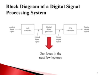
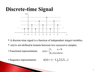
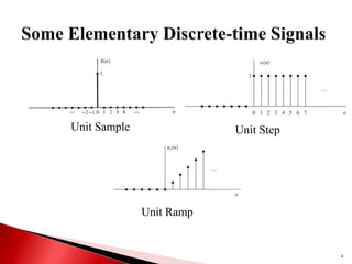
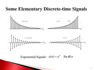
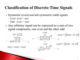
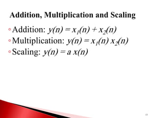
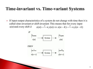
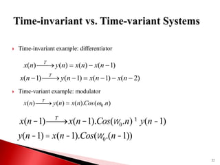
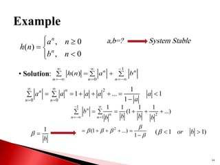
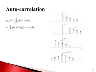
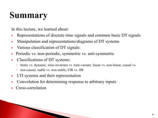
1) Discrete-time signals are functions of independent integer variables where samples are only defined at discrete time instants. 2) A discrete-time system transforms an input signal into an output signal through operations like addition, multiplication, delay. 3) Linear, time-invariant (LTI) systems have properties of superposition and time-invariance, and their behavior can be characterized by the impulse response. The output of an LTI system is the convolution of the input and impulse response.

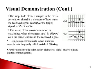
![ A discrete-time system is a device that performs some
operation on a discrete-time signal.
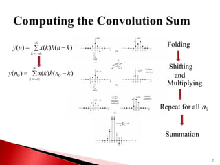
A system transforms an input signal x(n) into an output
signal y(n) where: .
Some basic discrete-time systems:
◦ Adders
◦ Constant multipliers
◦ Signal multipliers
◦ Unit delay elements
◦ Unit advance elements
9
)]
(
[
)
( n
x
T
n
y ](https://image.slidesharecdn.com/3-230125090805-e9e35c52/85/3-pdf-9-320.jpg)
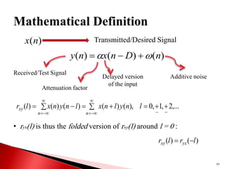
![14
elsewhere
,
0
3
3
,
)
(
n
n
n
x )]
1
(
)
(
)
1
(
[
3
1
)
(
n
x
n
x
n
x
n
y
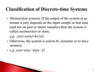
Moving average filter
}
0
,
3
,
2
,
1
,
0
,
1
,
2
,
3
,
0
{
)
(
n
x
Solution:
3
2
]
1
0
1
[
3
1
)]
1
(
)
0
(
)
1
(
[
3
1
)
0
(
x
x
x
y
}
0
,
1
,
3
5
,
2
,
1
,
3
2
,
1
,
2
,
3
5
,
1
,
0
{
)
(
n
y](https://image.slidesharecdn.com/3-230125090805-e9e35c52/85/3-pdf-14-320.jpg)
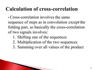
![15
elsewhere
,
0
3
3
,
)
(
n
n
n
x ...]
)
2
(
)
1
(
)
(
[
)
(
n
x
n
x
n
x
n
y
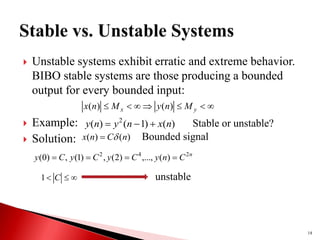
Accumulator
}
0
,
3
,
2
,
1
,
0
,
1
,
2
,
3
,
0
{
)
(
n
x
Solution:
}
12
,
12
,
9
,
7
,
6
,
6
,
5
,
3
,
0
{
)
(
n
y](https://image.slidesharecdn.com/3-230125090805-e9e35c52/85/3-pdf-15-320.jpg)
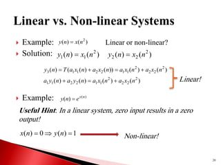
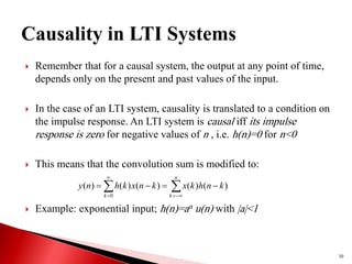
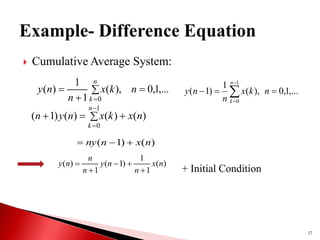
![ In a causal system, the output at any time n only
depends on the present and past inputs.
An example of a causal system:
y(n)=F[x(n),x(n−1),x(n− 2),...]
All other systems are non-causal.
A subset of non-causal system where the system
output, at any time n only depends on future inputs is
called anti-causal.
y(n)=F[x(n+1),x(n+2),...]
17](https://image.slidesharecdn.com/3-230125090805-e9e35c52/85/3-pdf-17-320.jpg)
![ Superposition principle:T[ax1(n)+bx2(n)]=aT[x1(n)]+bT[x2 (n)]
A relaxed linear system with zero input
produces a zero output.
19
Scaling property
Additivity property](https://image.slidesharecdn.com/3-230125090805-e9e35c52/85/3-pdf-19-320.jpg)
![ LTI systems have two important characteristics:
◦ Time invariance: A system T is called time-invariant or shift-
invariant if input-output characteristics of the system do not
change with time
◦ Linearity: A system T is called linear iff
Why do we care about LTI systems?
◦ Availability of a large collection of mathematical techniques
◦ Many practical systems are either LTI or can be approximated by LTI
systems.
23
)
(
)
(
)
(
)
( k
n
y
k
n
x
n
y
n
x T
T
T[ax1(n)+bx2(n)]=aT[x1(n)]+bT[x2 (n)]](https://image.slidesharecdn.com/3-230125090805-e9e35c52/85/3-pdf-23-320.jpg)
![ h(n): the response of the LTI system to the input unit sample
(n), i.e. h(n)=T((n))
An LTI system is completely characterized by a single impulse
response h(n).
y(n)=T[x(n)]= )
(
*
)
(
)
(
)
( n
h
n
x
k
n
h
k
x
k
Response of the system to the input
unit sample sequence at n=k
Convolution
sum
24](https://image.slidesharecdn.com/3-230125090805-e9e35c52/85/3-pdf-24-320.jpg)
![26
)
(
*
)
(
)
(
*
)
( n
x
n
h
n
h
n
x
• Commutative law:
)]
(
2
*
)
(
)
(
1
*
)
(
)]
(
2
)]
(
1
[
*
)
( n
h
n
x
n
h
n
x
n
h
n
h
n
x
Distributive law:](https://image.slidesharecdn.com/3-230125090805-e9e35c52/85/3-pdf-26-320.jpg)
![27
)]
(
2
*
)
(
1
[
*
)
(
)
(
2
*
)]
(
1
*
)
(
[ n
h
n
h
n
x
n
h
n
h
n
x
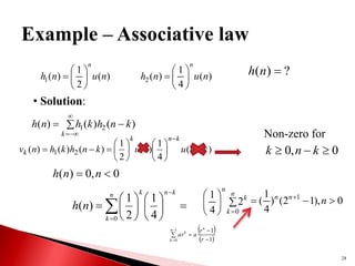
Associative law:](https://image.slidesharecdn.com/3-230125090805-e9e35c52/85/3-pdf-27-320.jpg)
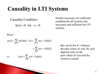
![33
Stability Condition : A linear time-invariant system is stable iff
k
x
k
k
k
h
B
k
n
x
k
h
k
n
x
k
h
n
y
a ]
[
]
[
]
[
]
[
]
[
]
[
:
cy)
(Sufficien
)
output
unbounded
]
[
]
[
]
[
]
[
]
0
[
0
]
[
0
0
]
[
]
[
]
[
]
[
values
input with
the
Take
.
that
assume
us
Let
:
)
(Necessity
)
2
*
h
k
k
h
S
k
h
k
h
k
h
k
x
y
n
h
n
h
n
h
n
h
n
x
S
b
Stability of LTI Systems
k
h k
h
S )
(](https://image.slidesharecdn.com/3-230125090805-e9e35c52/85/3-pdf-33-320.jpg)


![Digital Signal Processing[ECEG-3171]-Ch1_L03](https://cdn.slidesharecdn.com/ss_thumbnails/dspl3-180427094423-thumbnail.jpg?width=640&height=640&fit=bounds)