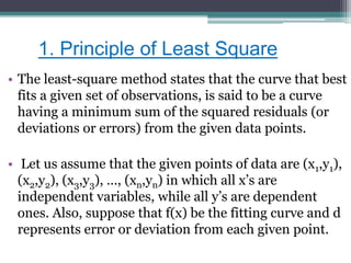
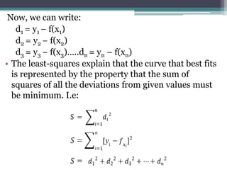
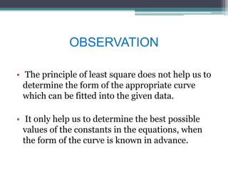
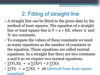
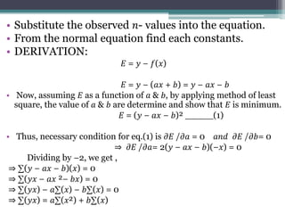
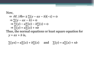
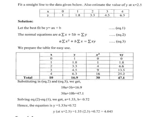
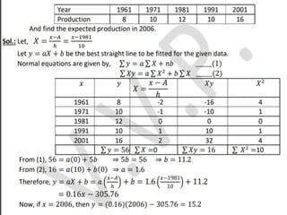
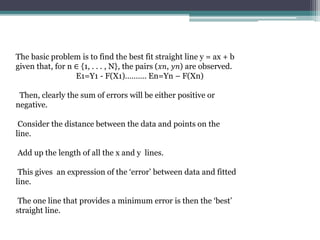
CURVE FITTING
Principle of least square
Fitting of a straight line
What is Curve Fitting?
• Curve fitting is the process of constructing a curve,
or mathematical function, that has the best fit to a
series of data points, possibly subject to
constraints.
Why Curve Fitting?
• The main purpose of curve fitting is to
theoretically describe experimental data with a
model (function or equation) and to find the
parameters associated with this model.
• Fitted curves can be used as an aid for data
visualization, to infer values of a function where
no data are available, and to summarize the
relationships among two or more variables
1. Principle of Least Square
• The least-square method states that the curve that best
fits a given set of observations, is said to be a curve
having a minimum sum of the squared residuals (or
deviations or errors) from the given data points.
• Let us assume that the given points of data are (x1,y1),
(x2,y2), (x3,y3), …, (xn,yn) in which all x’s are
independent variables, while all y’s are dependent
ones. Also, suppose that f(x) be the fitting curve and d
represents error or deviation from each given point.
Now, we can write:
d1 = y1 − f(x1)
d2 = y2 − f(x2)
d3 = y3 − f(x3)…..dn = yn – f(xn)
• The least-squares explain that the curve that best fits
is represented by the property that the sum of
squares of all the deviations from given values must
be minimum. I.e:
OBSERVATION
• The principle of least square does not help us to
determine the form of the appropriate curve
which can be fitted into the given data.
• It only help us to determine the best possible
values of the constants in the equations, when
the form of the curve is known in advance.
2. Fitting of straight line
• A straight line can be fitted to the given data by the
method of least squares. The equation of a straight
line or least square line is Y = a + bX, where ‘a’ and
‘b’ are constants.
• To compute the values of these constants we need
as many equations as the number of constants in
the equation. These equations are called normal
equations. In a straight line there are two constants
a and b so we require two normal equations.
• ∑(Yi,Xi) = 𝑎 ∑(Xi²) + 𝑏 ∑(Xi)
• ∑(Yi) = 𝑎 ∑(Xi) + 𝑛b (derived from least square
equation).
• Substitute the observed 𝑛- values into the equation.
• From the normal equation find each constants.
• DERIVATION:
𝐸 = 𝑦 − 𝑓(𝑥)
𝐸 = 𝑦 − (𝑎𝑥 + 𝑏) = 𝑦 − 𝑎𝑥 − 𝑏
• Now, assuming 𝐸 as a function of 𝑎 & 𝑏, by applying method of least
square, the value of 𝑎 & 𝑏 are determine and show that 𝐸 is minimum.
𝐸 = (𝑦 − 𝑎𝑥 − 𝑏)² _____(1)
• Thus, necessary condition for eq.(1) is 𝜕𝐸 /𝜕𝑎 = 0 𝑎𝑛𝑑 𝜕𝐸 /𝜕𝑏= 0
⇒ 𝜕𝐸 /𝜕𝑎= 2(𝑦 − 𝑎𝑥 − 𝑏)(−𝑥) = 0
Dividing by −2, we get ,
⇒ ∑(𝑦 − 𝑎𝑥 − 𝑏)(𝑥) = 0
⇒ ∑(𝑦𝑥 − 𝑎𝑥 ²− 𝑏𝑥) = 0
⇒ ∑(𝑦𝑥) − 𝑎∑(𝑥) − 𝑏∑(𝑥) = 0
⇒ ∑(𝑦𝑥) = 𝑎∑(𝑥²) + 𝑏∑(𝑥)
Now,
⇒ 𝜕𝐸 /𝜕b= 2 ∑(𝑦 − 𝑎𝑥 − 𝑏)(−1) = 0
⇒ ∑(𝑦 − 𝑎𝑥 − 𝑏) = 0
⇒ ∑(𝑦) − 𝑎∑(𝑥) − 𝑏∑(1) = 0
⇒ ∑(𝑦) = 𝑎∑(𝑥) + 𝑛𝑏
Thus, the normal equations or least square equation for
𝑦 = 𝑎𝑥 + 𝑏 is,
∑(𝑦𝑥) = 𝑎∑(𝑥) + 𝑏∑(𝑥) and ∑(𝑦) = 𝑎∑(𝑥) + 𝑛𝑏
To make the calculation easy of such large observation
there is another method to use for:
(1) If the no. of observations in the series of 𝑥 & 𝑦 are odd then the
assumed mean is,
𝑋 =𝑥 − 𝐴 𝑌 =𝑦 − 𝐴
h 𝑘
Where, 𝑨 = assumed mean of 𝑥, 𝒉 =class size(𝑥), 𝑩 =assumed
mean of 𝑦, 𝒌 =class size(𝑦)
(2) If the no. of observations are even in the series of 𝑥 & 𝑦, then
take arrange it in ascending order and take two middle most
observations and take average of it as a assumed mean.
i.e., A=Xi+Xi+1 th observation
2
THANK YOU
The basic problem is to find the best fit straight line y = ax + b
given that, for n ∈ {1, . . . , N}, the pairs (𝑥𝑛, 𝑦𝑛) are observed.
E1=Y1 - F(X1)………. En=Yn – F(Xn)
Then, clearly the sum of errors will be either positive or
negative.
Consider the distance between the data and points on the
line.
Add up the length of all the x and y lines.
This gives an expression of the ‘error’ between data and fitted
line.
The one line that provides a minimum error is then the ‘best’
straight line.

Curve fitting

  • 1.
    CURVE FITTING Principle ofleast square Fitting of a straight line
  • 2.
    What is CurveFitting? • Curve fitting is the process of constructing a curve, or mathematical function, that has the best fit to a series of data points, possibly subject to constraints.
  • 3.
    Why Curve Fitting? •The main purpose of curve fitting is to theoretically describe experimental data with a model (function or equation) and to find the parameters associated with this model. • Fitted curves can be used as an aid for data visualization, to infer values of a function where no data are available, and to summarize the relationships among two or more variables
  • 4.
    1. Principle ofLeast Square • The least-square method states that the curve that best fits a given set of observations, is said to be a curve having a minimum sum of the squared residuals (or deviations or errors) from the given data points. • Let us assume that the given points of data are (x1,y1), (x2,y2), (x3,y3), …, (xn,yn) in which all x’s are independent variables, while all y’s are dependent ones. Also, suppose that f(x) be the fitting curve and d represents error or deviation from each given point.
  • 5.
    Now, we canwrite: d1 = y1 − f(x1) d2 = y2 − f(x2) d3 = y3 − f(x3)…..dn = yn – f(xn) • The least-squares explain that the curve that best fits is represented by the property that the sum of squares of all the deviations from given values must be minimum. I.e:
  • 6.
    OBSERVATION • The principleof least square does not help us to determine the form of the appropriate curve which can be fitted into the given data. • It only help us to determine the best possible values of the constants in the equations, when the form of the curve is known in advance.
  • 7.
    2. Fitting ofstraight line • A straight line can be fitted to the given data by the method of least squares. The equation of a straight line or least square line is Y = a + bX, where ‘a’ and ‘b’ are constants. • To compute the values of these constants we need as many equations as the number of constants in the equation. These equations are called normal equations. In a straight line there are two constants a and b so we require two normal equations. • ∑(Yi,Xi) = 𝑎 ∑(Xi²) + 𝑏 ∑(Xi) • ∑(Yi) = 𝑎 ∑(Xi) + 𝑛b (derived from least square equation).
  • 8.
    • Substitute theobserved 𝑛- values into the equation. • From the normal equation find each constants. • DERIVATION: 𝐸 = 𝑦 − 𝑓(𝑥) 𝐸 = 𝑦 − (𝑎𝑥 + 𝑏) = 𝑦 − 𝑎𝑥 − 𝑏 • Now, assuming 𝐸 as a function of 𝑎 & 𝑏, by applying method of least square, the value of 𝑎 & 𝑏 are determine and show that 𝐸 is minimum. 𝐸 = (𝑦 − 𝑎𝑥 − 𝑏)² _____(1) • Thus, necessary condition for eq.(1) is 𝜕𝐸 /𝜕𝑎 = 0 𝑎𝑛𝑑 𝜕𝐸 /𝜕𝑏= 0 ⇒ 𝜕𝐸 /𝜕𝑎= 2(𝑦 − 𝑎𝑥 − 𝑏)(−𝑥) = 0 Dividing by −2, we get , ⇒ ∑(𝑦 − 𝑎𝑥 − 𝑏)(𝑥) = 0 ⇒ ∑(𝑦𝑥 − 𝑎𝑥 ²− 𝑏𝑥) = 0 ⇒ ∑(𝑦𝑥) − 𝑎∑(𝑥) − 𝑏∑(𝑥) = 0 ⇒ ∑(𝑦𝑥) = 𝑎∑(𝑥²) + 𝑏∑(𝑥)
  • 9.
    Now, ⇒ 𝜕𝐸 /𝜕b=2 ∑(𝑦 − 𝑎𝑥 − 𝑏)(−1) = 0 ⇒ ∑(𝑦 − 𝑎𝑥 − 𝑏) = 0 ⇒ ∑(𝑦) − 𝑎∑(𝑥) − 𝑏∑(1) = 0 ⇒ ∑(𝑦) = 𝑎∑(𝑥) + 𝑛𝑏 Thus, the normal equations or least square equation for 𝑦 = 𝑎𝑥 + 𝑏 is, ∑(𝑦𝑥) = 𝑎∑(𝑥) + 𝑏∑(𝑥) and ∑(𝑦) = 𝑎∑(𝑥) + 𝑛𝑏
  • 11.
    To make thecalculation easy of such large observation there is another method to use for: (1) If the no. of observations in the series of 𝑥 & 𝑦 are odd then the assumed mean is, 𝑋 =𝑥 − 𝐴 𝑌 =𝑦 − 𝐴 h 𝑘 Where, 𝑨 = assumed mean of 𝑥, 𝒉 =class size(𝑥), 𝑩 =assumed mean of 𝑦, 𝒌 =class size(𝑦) (2) If the no. of observations are even in the series of 𝑥 & 𝑦, then take arrange it in ascending order and take two middle most observations and take average of it as a assumed mean. i.e., A=Xi+Xi+1 th observation 2
  • 13.
  • 14.
    The basic problemis to find the best fit straight line y = ax + b given that, for n ∈ {1, . . . , N}, the pairs (𝑥𝑛, 𝑦𝑛) are observed. E1=Y1 - F(X1)………. En=Yn – F(Xn) Then, clearly the sum of errors will be either positive or negative. Consider the distance between the data and points on the line. Add up the length of all the x and y lines. This gives an expression of the ‘error’ between data and fitted line. The one line that provides a minimum error is then the ‘best’ straight line.