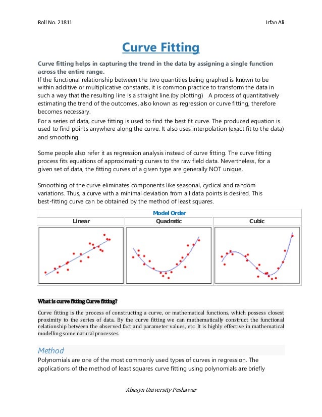
The document discusses curve fitting, which is the process of constructing mathematical functions to closely approximate a set of data points. It explains methods such as linear regression and polynomial fitting, particularly emphasizing the least squares method for finding the best fit. Additionally, it illustrates various examples and applications of curve fitting in predicting outcomes and analyzing trends.

1. Roll No. 21811 Irfan Ali
Abasyn University Peshawar
Curve Fitting
Curve fitting helps in capturing the trend in the data by assigning a single function
across the entire range.
If the functional relationship between the two quantities being graphed is known to be
within additive or multiplicative constants, it is common practice to transform the data in
such a way that the resulting line is a straight line.(by plotting) A process of quantitatively
estimating the trend of the outcomes, also known as regression or curve fitting, therefore
becomes necessary.
For a series of data, curve fitting is used to find the best fit curve. The produced equation is
used to find points anywhere along the curve. It also uses interpolation (exact fit to the data)
and smoothing.
Some people also refer it as regression analysis instead of curve fitting. The curve fitting
process fits equations of approximating curves to the raw field data. Nevertheless, for a
given set of data, the fitting curves of a given type are generally NOT unique.
Smoothing of the curve eliminates components like seasonal, cyclical and random
variations. Thus, a curve with a minimal deviation from all data points is desired. This
best-fitting curve can be obtained by the method of least squares.
Model Order
Linear Quadratic Cubic
What is curve fitting Curve fitting?
Curve fitting is the process of constructing a curve, or mathematical functions, which possess closest
proximity to the series of data. By the curve fitting we can mathematically construct the functional
relationship between the observed fact and parameter values, etc. It is highly effective in mathematical
modelling some natural processes.
Method
Polynomials are one of the most commonly used types of curves in regression. The
applications of the method of least squares curve fitting using polynomials are briefly

2. Roll No. 21811 Irfan Ali
Abasyn University Peshawar
discussed.
Commonly used method for curve fitting are least square curve fits and nonlinear
curve fits:
Least square curve fits: The linear least squares fitting technique is the simplest and
most commonly applied form of linear regression and provides a solution to the
problem of finding the best fitting straight line through a set of points. The trend
equation can be used to predict the values of the variable for any period t in future or even
in intermediate periods of the given series and the forecasted values are also quite reliable.
One of the simplest and most commonly used form of linear regression.
Principle under least squares is it minimizes the square of the error between the original
data and the values predicted by the equation.
This method is sensitive to outliers in the data. Through a set of points we can find the
best fitting straight line.
Let the data points be (l1,m1),(l2,m2),.........(ln, mn )
l being the independent variable and m the dependent variable. The fitting curve is said to
have a deviation d from each data point
d1=m1−f(l1), d2=m2−f(l2),...........dn = mn−f(ln),
→ π = d21+d22+.........+d2n =∑ni=1 d2
i
= ∑ni=1[mi−f(li)]2
= Minimum
How to do Curve Fitting?
Given below are some of the equations explained which are used frequently for curve fitting.
Fitting of linear trend:
Consider a straight line trend between the given time series value (y) and time (t)
y = a + bt ......(*)
For any time t, the estimated value ye of y is
ye = a + bt

3. Roll No. 21811 Irfan Ali
Abasyn University Peshawar
Estimate the values of a and b
E = ∑ (y - ye)2
= ∑(y - a - bt)2
Is minimum
The summation is taken over the given value of time series:
∂E/∂a = 0
= −2∑(y−a−bt)−2∑(y−a−bt)
∂E/∂b = 0
= −2∑t(y−a−b t)−2∑t(y−a−bt)
On simplification of the above equations we get the normal equations for estimating a and
b
∑y= n a + b ∑t ∑ty= a ∑t +b ∑t2 ∑y= n a + b ∑t ∑ty = a ∑t + b ∑t2
n : number of time series pairs(t,y)
Solve the above two equations for a and b and substitute these values in *
Then you finally get the equation of the straight line trend.
Fitting of Exponential trend:
Exponential curve equation is of the form
y = a bt
Take logarithm on both sides
log y = log a + t log b
→ Y = A + Bt
Y = log y; A = log a and B = log b .......... *
The normal equations for estimating A and B are
∑ Y = n A + B ∑ t
and ∑ t Y = A ∑ t + B ∑ t2
The above equations can be solved for A and B, and on using * we get
a = Antilog (A)

4. Roll No. 21811 Irfan Ali
Abasyn University Peshawar
b = Antilog (B)
With the values of a and b, the curve becomes best exponential trend curve.
Second Degree Curve fitting to logarithms:
Suppose the trend curve is of the type
y = a bt ct^2
Take logarithm on both sides
log y = log a + t log b + t{2}
log c
Y = A + B t + C t2
Y = log y; A = log a, B = log b, C = log c
A second degree parabolic curve in Y and t can be fitted now.
So we get a = Antilog(A); b = Antilog(B) and c = Antilog(C)
With these values of a, b and c the curve becomes the best second degree curve fitted to
logarithms.
Examples
Some numerical examples to illustrate the technique of curve fitting are given below:
Example 1: The linear trend of sales of a company is $$ 6, 50, 000 in 1995 and it rises
by $$16,500 per year.
Write the trend equation, if the company knows that its sales in 1998 will be 10% below the
forecasted trend sales, find its expected sales in 1998.
Solution: The sales of the company are $ 650000 in 1995 and they exhibit a linear trend
with a constant rise of $ 16,500 per year.
The annual trend equation of the sales of the company is
Y = 650000 + 16500 t
Yt : Annual sales in $;
t units = 1 year
The estimated sales of the company in 1998 when t = 3 is
(Yt)1998 = $ (650000+16500 x 3)
= $(650000 + 49500)
= $ 699500

5. Roll No. 21811 Irfan Ali
Abasyn University Peshawar
Actual sales in 1998 = $[699500 – (10/100)x (699500)]
= $(699500 - 69950)
= $629550
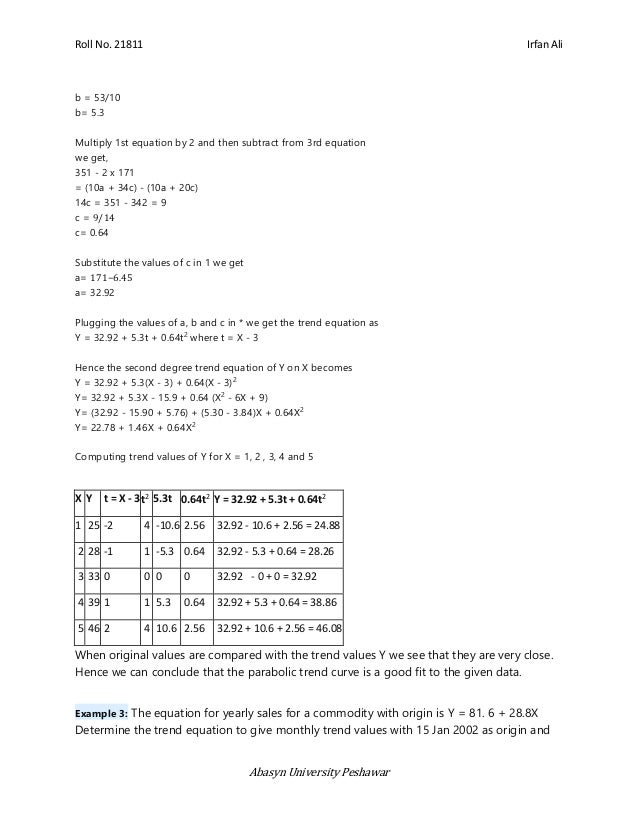
Example 2: Fit an equation of the form Y = a + bX + cX2 to the data given below
X 1 2 3 4 5
Y 2528 3339 46
Solution : As n : The number of pairs is odd
we take t = X - (Middle value) = X -
The values of t corresponding to X = 1, 2, 3, 4 and 5 are -2, -1, 0, 1 and 2 respectively.
Let the second degree trend equation between Y and t be
Y = a + bt + ct2
where t = X - 3 ........(*)
Second Degree Terms:
X Y t = X - 3 t2 t3 t4 t Y t2
Y
1 25 -2 4 -8 16 -50 100
2 28 -1 1 -1 1 -28 28
3 33 0 0 0 0 0 0
4 39 1 1 1 1 39 39
5 46 2 4 8 16 92 184
Total∑ y = 171 ∑ t2
= 10 ∑ t3
=0 ∑ t4
=34∑t Y = 53 ∑ t2
Y = 351
Now the normal equations for estimating a, b and c are
∑y = na + b ∑ t + c ∑ t2
∑ t y = a ∑ t + b ∑ t2
+ c ∑ t3
∑t2
y = a ∑ t2
+ b ∑ t3
+ c ∑ t4
171 = 5a + 10c ..........1
53 = 10b .......... 2
351 = 10a + 34c ......... 3

6. Roll No. 21811 Irfan Ali
Abasyn University Peshawar
b = 53/10
b= 5.3
Multiply 1st equation by 2 and then subtract from 3rd equation
we get,
351 - 2 x 171
= (10a + 34c) - (10a + 20c)
14c = 351 - 342 = 9
c = 9/14
c= 0.64
Substitute the values of c in 1 we get
a= 171−6.45
a= 32.92
Plugging the values of a, b and c in * we get the trend equation as
Y = 32.92 + 5.3t + 0.64t2
where t = X - 3
Hence the second degree trend equation of Y on X becomes
Y = 32.92 + 5.3(X - 3) + 0.64(X - 3)2
Y= 32.92 + 5.3X - 15.9 + 0.64 (X2
- 6X + 9)
Y= (32.92 - 15.90 + 5.76) + (5.30 - 3.84)X + 0.64X2
Y= 22.78 + 1.46X + 0.64X2
Computing trend values of Y for X = 1, 2 , 3, 4 and 5
X Y t = X - 3t2 5.3t 0.64t2
Y = 32.92 + 5.3t + 0.64t2
1 25 -2 4 -10.6 2.56 32.92 - 10.6 + 2.56 = 24.88
2 28 -1 1 -5.3 0.64 32.92 - 5.3 + 0.64 = 28.26
3 33 0 0 0 0 32.92 - 0 + 0 = 32.92
4 39 1 1 5.3 0.64 32.92 + 5.3 + 0.64 = 38.86
5 46 2 4 10.6 2.56 32.92 + 10.6 + 2.56 = 46.08
When original values are compared with the trend values Y we see that they are very close.
Hence we can conclude that the parabolic trend curve is a good fit to the given data.
Example 3: The equation for yearly sales for a commodity with origin is Y = 81. 6 + 28.8X
Determine the trend equation to give monthly trend values with 15 Jan 2002 as origin and

7. Roll No. 21811 Irfan Ali
Abasyn University Peshawar
Calculate the trend values for March 2002 to August 2002.
Solution: The given annual trend equation reduced to monthly values becomes
ye = 81.612 + 28.8144 x
= 6.8 + 0.2 x
We need to shift the origin to January 2002 , shift the origin 6 1212 months forward and
the required equation is obtained on changing x to x + 6.5.
Hence new trend equation is given by
ye = 6.8 + 0.2 (x + 6.5)
= 6.8 + 0.2x + 1.3
= 8.1 + 0.2x .......( *)
x unit = 1 month
y unit = Average monthly sales
The trend values for middle of march 2002 to middle of August 2002 are obtained on taking
x = 2, 3, 4, 5, 6, 7 respectively in * and are given in the table below.
Month x ye = 8.1 + 0.2x ye (in $$)
March 2 8.1 + 0.2 * 2 = 8.5 8500
April 3 8.1 + 0.2 * 3 =8.7 8700
May 4 8.1 + 0.2 * 4 =8.9 8900
June 5 8.1 + 0.2 * 5 =9.1 9100
July 6 8.1 + 0.2 * 6 =9.3 9300
August 7 8.1 + 0.2 * 7 =9.5 9500
What is fitting a model?
Model fitting is a procedure that takes three steps: First you need a function that takes
in a set of parameters and returns a predicted data set. Second you need an 'error
function' that provides a number representing the difference between your data and
the model's prediction for any given set of model parameters.

8. Roll No. 21811 Irfan Ali
Abasyn University Peshawar
What is a fitting model?
A fit model (sometimes fitting model) is a person who is used by a fashion designer or
clothing manufacturer to check the fit, drape and visual appearance of a design on a
'real' human being, effectively acting as a live mannequin.
What is a model fit statistics?
The goodness of fit of a statistical model describes how well it fits a set of
observations. Measures of goodness of fit typically summarize the discrepancy
between observed values and the values expected under the model in question.
What is a commercial model?
Commercial modeling is a more generalized type of modeling. There are high
fashion models, and then there are commercial models. ... They can model for
television, commercials, websites, magazines, newspapers, billboards and any other
type of advertisement. Most people who tell you they are models are “commercial”
models.
What is the exponential growth curve?
Growth of a system in which the amount being added to the system is proportional to the
amount already present: the bigger the system is, the greater the increase. ( See geometric
progression.) Note : In everyday speech, exponential growth means runaway expansion, such
as in population growth.
Why is population exponential?
Exponential population growth: When resources are unlimited, populations
exhibit exponential growth, resulting in a J-shaped curve. When resources are
limited, populations exhibit logistic growth. In logistic growth, population expansion
decreases as resources become scarce.
What is the logistic growth model?
A typical application of the logistic equation is a common model of population
growth (see also population dynamics), originally due to Pierre-François Verhulst in
1838, where the rate of reproduction is proportional to both the existing population and
the amount of available resources, all else being equal.
What is the difference between linear and exponential growth?
Question: Describe the basic differences between linear growth and exponential
growth. ... Linear growth occurs when a quantity grows by the same relative amount,
that is, by the same percentage, in each unit of time, and exponential growth occurs
when a quantity grows by the same absolute amount in each unit of time.