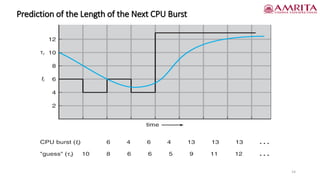
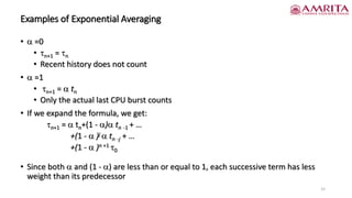
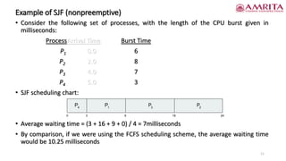
Amrita
School
of
Engineering,
Bangalore
Ms. Harika Pudugosula
Teaching Assistant
Department of Electronics & Communication Engineering
• Basic Concepts
• Scheduling Criteria
• Scheduling Algorithms
2
3
Scheduling
• Example:
4
Scheduling Algorithm Optimization Criteria
• Max CPU utilization - keep CPU as busy as possible
• Max throughput - Number of processes that complete their execution
per time unit
• Min turnaround time - amount of time to execute a particular process
• Min waiting time - amount of time that a process spends waiting in the
ready queue
• Min response time - amount of time it takes from when a request was
submitted until the first response is produced, not output (for time-
sharing environment)
Scheduling Algorithms
First- Come, First-Served (FCFS) Scheduling
• By far the simplest CPU-scheduling algorithm is the first-come, first-served (FCFS)
scheduling algorithm
• The process that requests the CPU first is allocated the CPU first
• The implementation of the FCFS policy is easily managed with a FIFO queue
• When a process enters the ready queue, its PCB is linked onto the tail of the queue
• When the CPU is free, it is allocated to the process at the head of the queue
• The running process is then removed from the queue
6
First- Come, First-Served (FCFS) Scheduling
Process Burst Time
P1 24
P2 3
P3 3
• Suppose that the processes arrive in the order: P1 , P2 , P3
The Gantt Chart for the schedule is:
• Waiting time for P1 = 0ms ; P2 = 24ms ; P3 = 27ms
• Average waiting time: (0 + 24 + 27)/3 = 17ms
P P P
1 2 3
0 24 30
27
7
FCFS Scheduling (Cont.)
Suppose that the processes arrive in the order:
P2 , P3 , P1
The Gantt chart for the schedule is:
Waiting time for P1 = 6ms ;P2 = 0ms; P3 = 3ms
Average waiting time: (6 + 0 + 3)/3 = 3ms
This reduction is substantial. Thus, the average waiting time under an FCFS policy is
generally not minimal and may vary substantially if the processes’ CPU burst times
vary greatly
P1
0 3 6 30
P2
P3
8
FCFS Scheduling (Cont.)
• Much better than previous case
• The FCFS scheduling algorithm is nonpremptive
• Once the CPU has been allocated to a process, that process keeps the CPU until it
releases the CPU, either by terminating or by requesting I/O
• The FCFS algorithm is thus particularly troublesome for time-sharing systems, where it
is important that each user get a share of the CPU at regular intervals
• It would be disastrous to allow one process to keep the CPU for an extended period
Convoy effect - short process behind long process
Consider one CPU-bound and many I/O-bound processes
9
Shortest-Job-First (SJF) Scheduling
• This algorithm associates with each process the length of the process’s next CPU
burst i.e., the process which has least next CPU burst time will be assigned to CPU
• If the next CPU bursts of two processes are the same, FCFS scheduling is used to
break the tie
• The SJF algorithm can be either preemptive or nonpreemptive
• Scheduling depends on the length of the next CPU burst of a process, rather than its
total length - Shortest-next CPU-burst algorithm
• SJF is optimal – gives minimum average waiting time for a given set of processes
• The difficulty is knowing the length of the next CPU request
• Could ask the user
10
Example of SJF (nonpreemptive)
• Consider the following set of processes, with the length of the CPU burst given in
milliseconds:
ProcessArrival Time Burst Time
P1 0.0 6
P2 2.0 8
P3 4.0 7
P4 5.0 3
• SJF scheduling chart:
• Average waiting time = (3 + 16 + 9 + 0) / 4 = 7milliseconds
• By comparison, if we were using the FCFS scheduling scheme, the average waiting time
would be 10.25 milliseconds
P3
0 3 24
P4
P1
16
9
P2
11
Example of Shortest-remaining-time-first / Preemptive SJF Scheduling
Now we add the concepts of varying arrival times and preemption to the analysis
Process Arrival Time(ms)Burst Time(ms)
P1 0 8
P2 1 4
P3 2 9
P4 3 5
Preemptive SJF Gantt Chart
Average waiting time = [(10-1)+(1-1)+(17-2)+5-3)]/4 = 26/4 = 6.5 msec
P4
0 1 26
P1
P2
10
P3
P1
5 17
12
Determining Length of Next CPU Burst
Can only estimate the length – should be similar to the previous one
Then pick process with shortest predicted next CPU burst
Can be done by using the length of previous CPU bursts, using exponential averaging
Commonly, α set to ½
Preemptive version called shortest-remaining-time-first
:
Define
4.
1
0
,
3.
burst
CPU
next
the
for
value
predicted
2.
burst
CPU
of
length
actual
1.


=
=
+


 1
n
th
n n
t
( ) .
1
1 n
n
n
t 


 −
+
=
=
13
Prediction of the Length of the Next CPU Burst
14
Examples of Exponential Averaging
•  =0
• n+1 = n
• Recent history does not count
•  =1
• n+1 =  tn
• Only the actual last CPU burst counts
• If we expand the formula, we get:
n+1 =  tn+(1 - ) tn -1 + …
+(1 -  )j  tn -j + …
+(1 -  )n +1 0
• Since both  and (1 - ) are less than or equal to 1, each successive term has less
weight than its predecessor
15
16
References
1. Silberscatnz and Galvin, “Operating System Concepts,” Ninth Edition, John
Wiley and Sons, 2012.
17
Thank you

CPU Scheduling Part-II.pdf

  • 1.
    Amrita School of Engineering, Bangalore Ms. Harika Pudugosula TeachingAssistant Department of Electronics & Communication Engineering
  • 2.
    • Basic Concepts •Scheduling Criteria • Scheduling Algorithms 2
  • 3.
  • 4.
    4 Scheduling Algorithm OptimizationCriteria • Max CPU utilization - keep CPU as busy as possible • Max throughput - Number of processes that complete their execution per time unit • Min turnaround time - amount of time to execute a particular process • Min waiting time - amount of time that a process spends waiting in the ready queue • Min response time - amount of time it takes from when a request was submitted until the first response is produced, not output (for time- sharing environment)
  • 5.
  • 6.
    First- Come, First-Served(FCFS) Scheduling • By far the simplest CPU-scheduling algorithm is the first-come, first-served (FCFS) scheduling algorithm • The process that requests the CPU first is allocated the CPU first • The implementation of the FCFS policy is easily managed with a FIFO queue • When a process enters the ready queue, its PCB is linked onto the tail of the queue • When the CPU is free, it is allocated to the process at the head of the queue • The running process is then removed from the queue 6
  • 7.
    First- Come, First-Served(FCFS) Scheduling Process Burst Time P1 24 P2 3 P3 3 • Suppose that the processes arrive in the order: P1 , P2 , P3 The Gantt Chart for the schedule is: • Waiting time for P1 = 0ms ; P2 = 24ms ; P3 = 27ms • Average waiting time: (0 + 24 + 27)/3 = 17ms P P P 1 2 3 0 24 30 27 7
  • 8.
    FCFS Scheduling (Cont.) Supposethat the processes arrive in the order: P2 , P3 , P1 The Gantt chart for the schedule is: Waiting time for P1 = 6ms ;P2 = 0ms; P3 = 3ms Average waiting time: (6 + 0 + 3)/3 = 3ms This reduction is substantial. Thus, the average waiting time under an FCFS policy is generally not minimal and may vary substantially if the processes’ CPU burst times vary greatly P1 0 3 6 30 P2 P3 8
  • 9.
    FCFS Scheduling (Cont.) •Much better than previous case • The FCFS scheduling algorithm is nonpremptive • Once the CPU has been allocated to a process, that process keeps the CPU until it releases the CPU, either by terminating or by requesting I/O • The FCFS algorithm is thus particularly troublesome for time-sharing systems, where it is important that each user get a share of the CPU at regular intervals • It would be disastrous to allow one process to keep the CPU for an extended period Convoy effect - short process behind long process Consider one CPU-bound and many I/O-bound processes 9
  • 10.
    Shortest-Job-First (SJF) Scheduling •This algorithm associates with each process the length of the process’s next CPU burst i.e., the process which has least next CPU burst time will be assigned to CPU • If the next CPU bursts of two processes are the same, FCFS scheduling is used to break the tie • The SJF algorithm can be either preemptive or nonpreemptive • Scheduling depends on the length of the next CPU burst of a process, rather than its total length - Shortest-next CPU-burst algorithm • SJF is optimal – gives minimum average waiting time for a given set of processes • The difficulty is knowing the length of the next CPU request • Could ask the user 10
  • 11.
    Example of SJF(nonpreemptive) • Consider the following set of processes, with the length of the CPU burst given in milliseconds: ProcessArrival Time Burst Time P1 0.0 6 P2 2.0 8 P3 4.0 7 P4 5.0 3 • SJF scheduling chart: • Average waiting time = (3 + 16 + 9 + 0) / 4 = 7milliseconds • By comparison, if we were using the FCFS scheduling scheme, the average waiting time would be 10.25 milliseconds P3 0 3 24 P4 P1 16 9 P2 11
  • 12.
    Example of Shortest-remaining-time-first/ Preemptive SJF Scheduling Now we add the concepts of varying arrival times and preemption to the analysis Process Arrival Time(ms)Burst Time(ms) P1 0 8 P2 1 4 P3 2 9 P4 3 5 Preemptive SJF Gantt Chart Average waiting time = [(10-1)+(1-1)+(17-2)+5-3)]/4 = 26/4 = 6.5 msec P4 0 1 26 P1 P2 10 P3 P1 5 17 12
  • 13.
    Determining Length ofNext CPU Burst Can only estimate the length – should be similar to the previous one Then pick process with shortest predicted next CPU burst Can be done by using the length of previous CPU bursts, using exponential averaging Commonly, α set to ½ Preemptive version called shortest-remaining-time-first : Define 4. 1 0 , 3. burst CPU next the for value predicted 2. burst CPU of length actual 1.   = = +    1 n th n n t ( ) . 1 1 n n n t     − + = = 13
  • 14.
    Prediction of theLength of the Next CPU Burst 14
  • 15.
    Examples of ExponentialAveraging •  =0 • n+1 = n • Recent history does not count •  =1 • n+1 =  tn • Only the actual last CPU burst counts • If we expand the formula, we get: n+1 =  tn+(1 - ) tn -1 + … +(1 -  )j  tn -j + … +(1 -  )n +1 0 • Since both  and (1 - ) are less than or equal to 1, each successive term has less weight than its predecessor 15
  • 16.
    16 References 1. Silberscatnz andGalvin, “Operating System Concepts,” Ninth Edition, John Wiley and Sons, 2012.
  • 17.