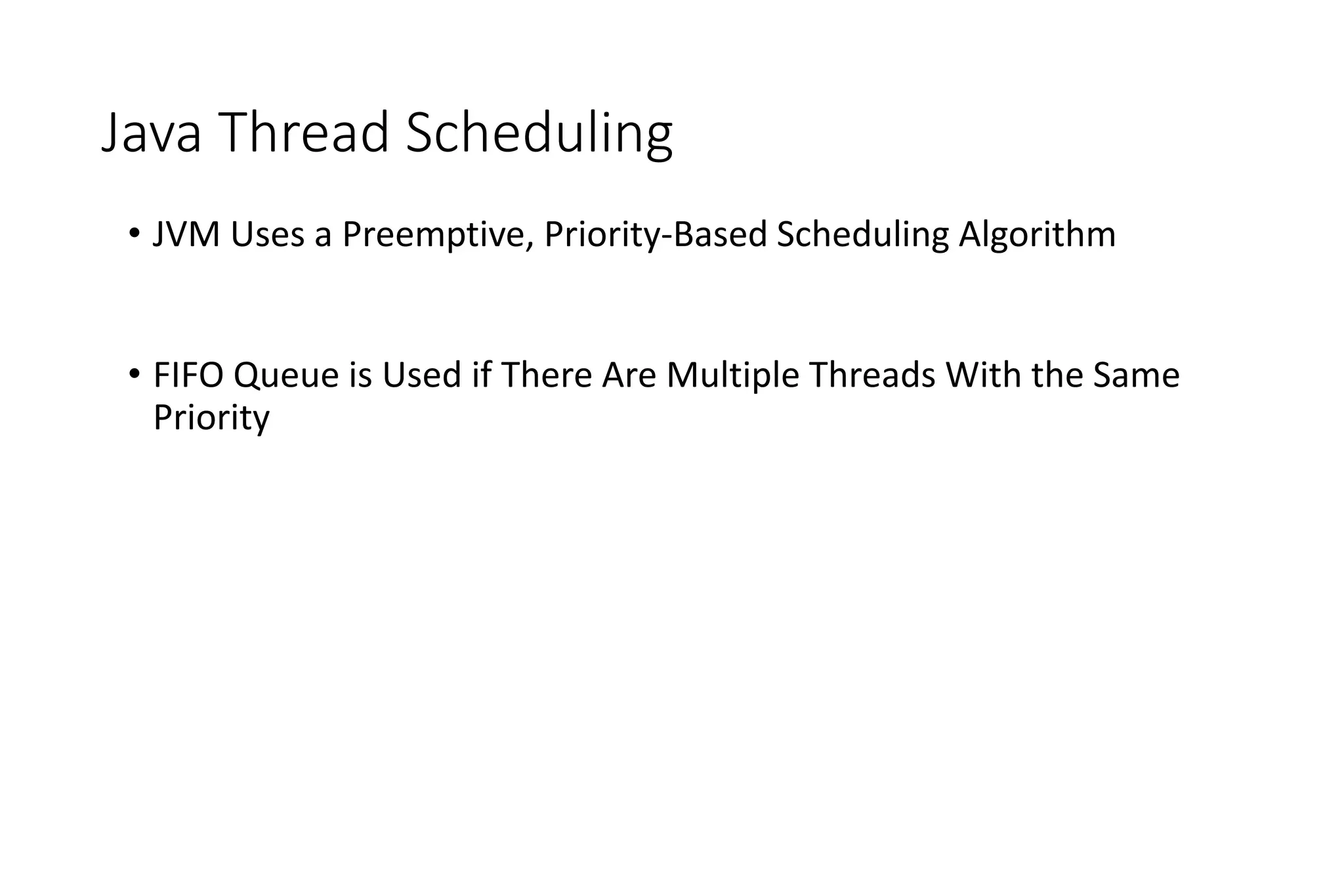
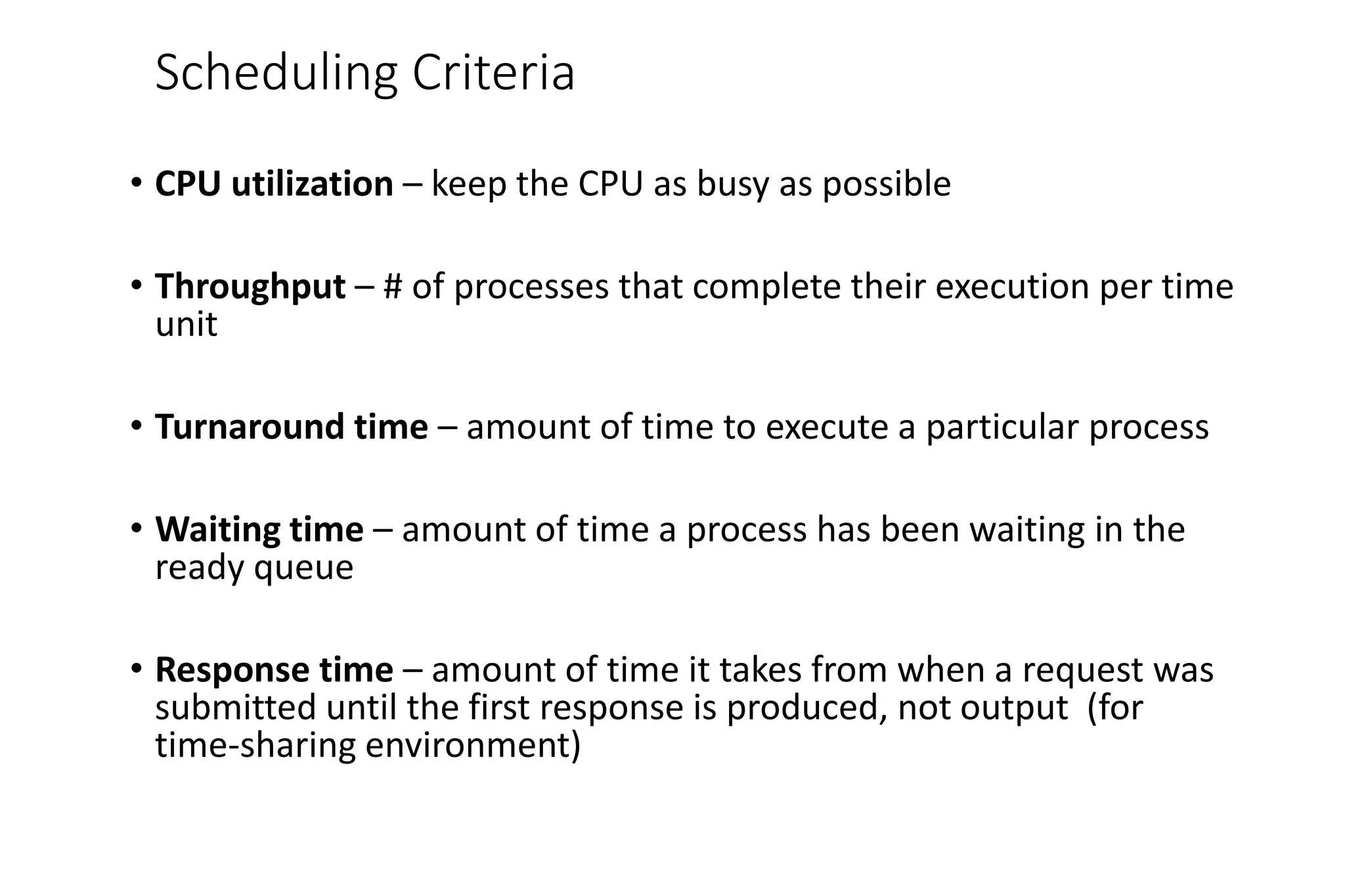
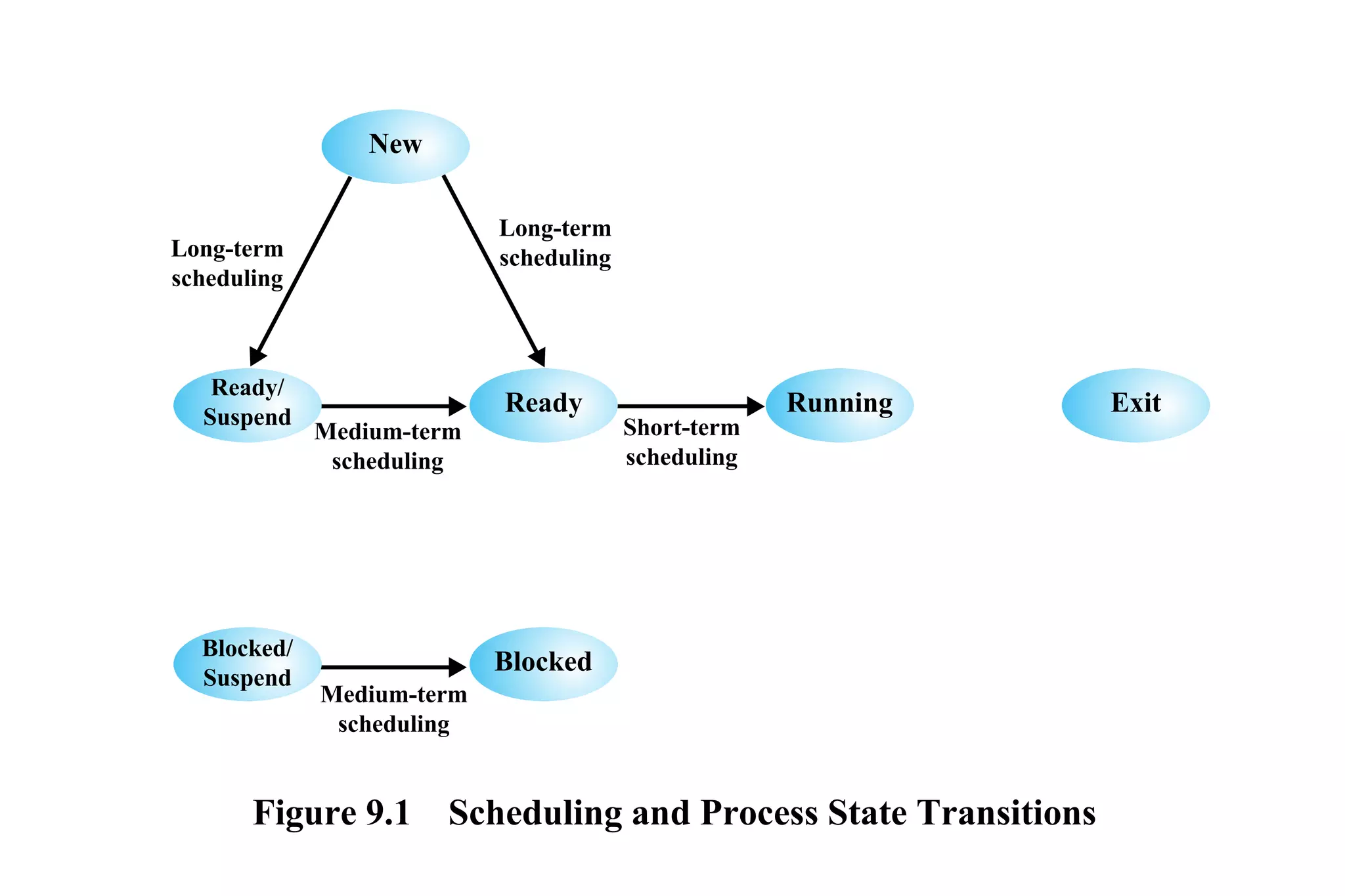
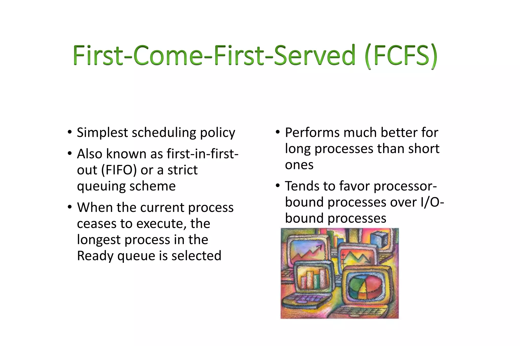
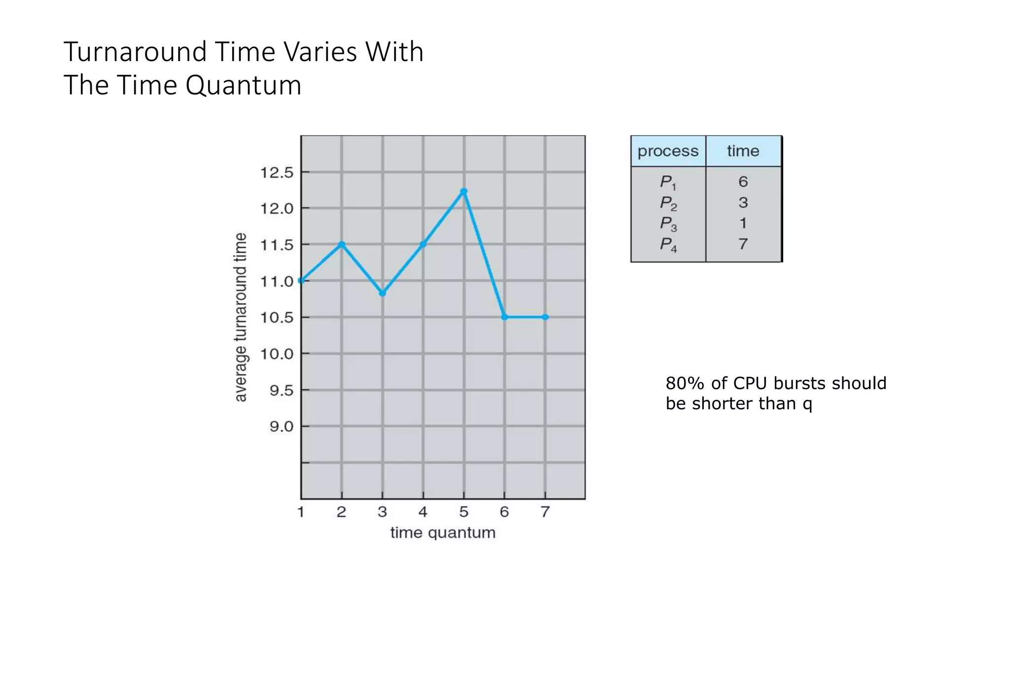
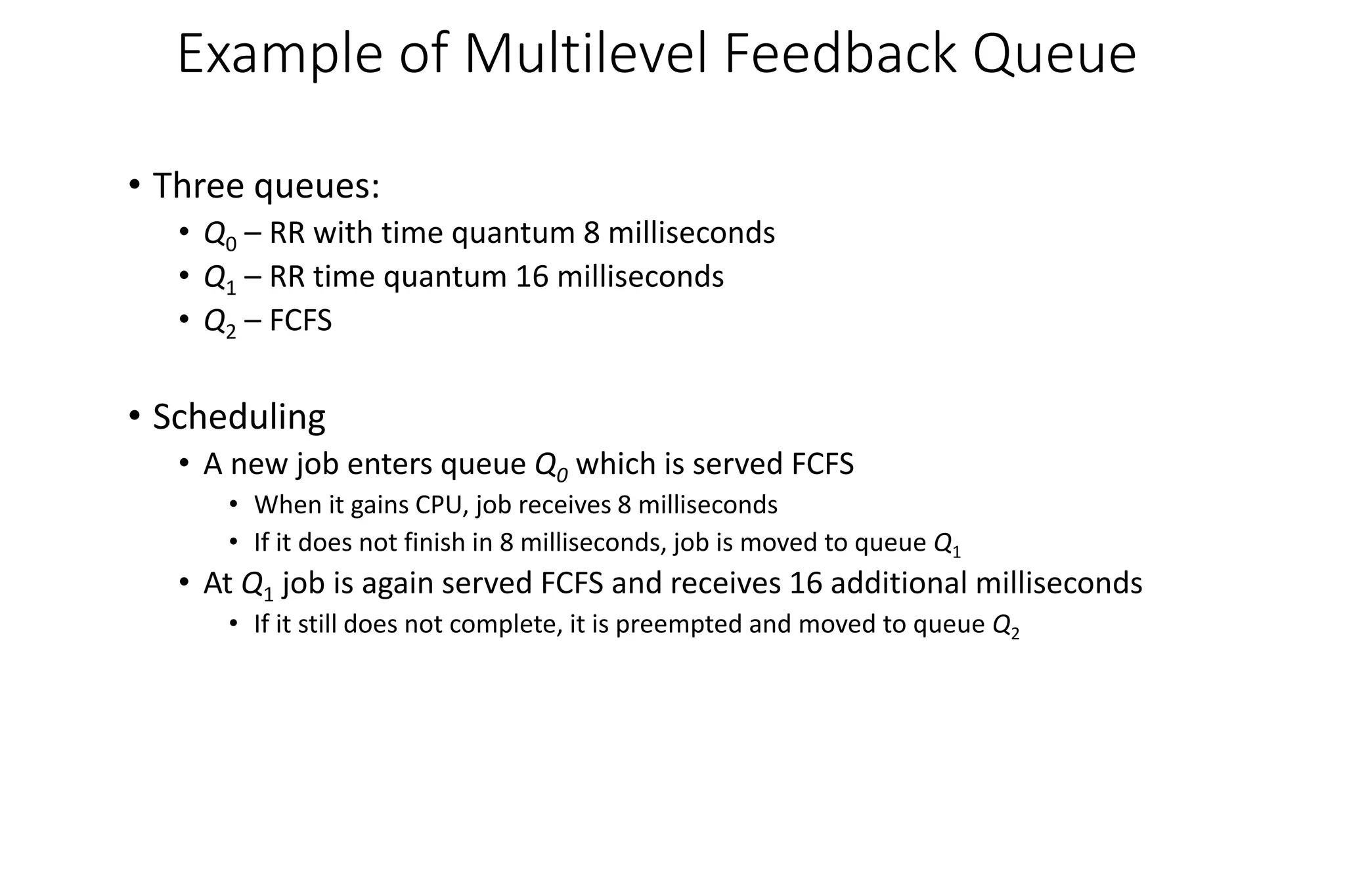
CPU scheduling determines which process will be assigned to the CPU for execution. There are several types of scheduling algorithms:
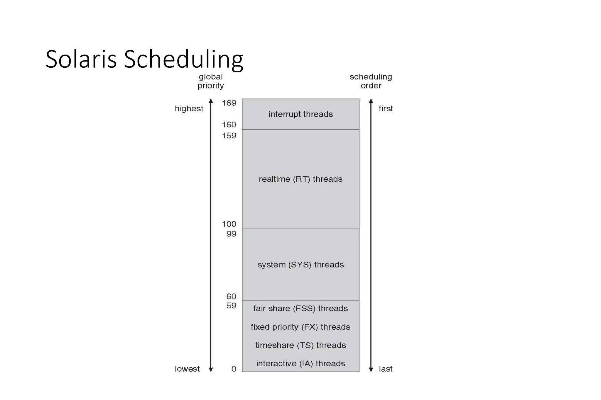
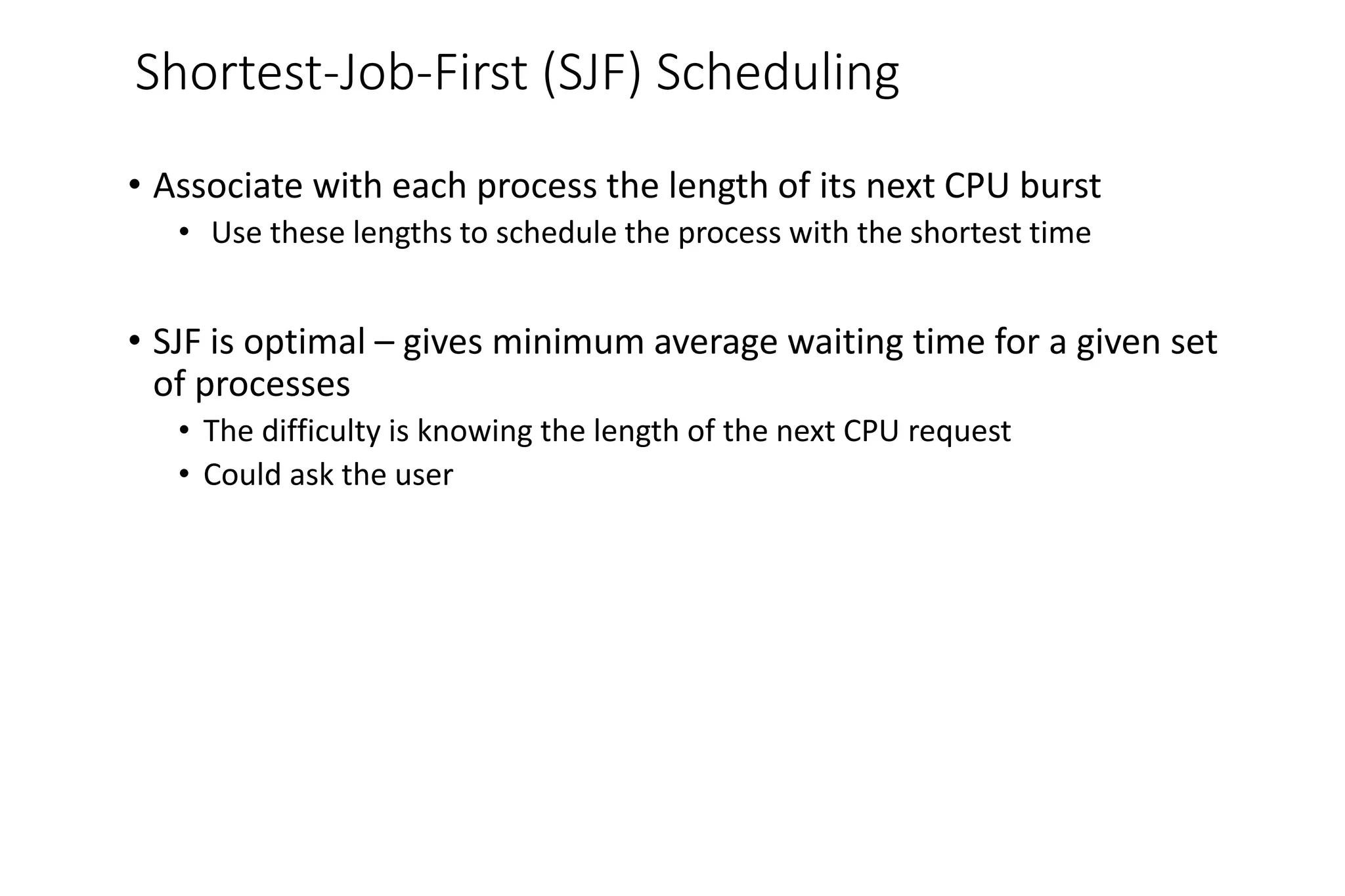
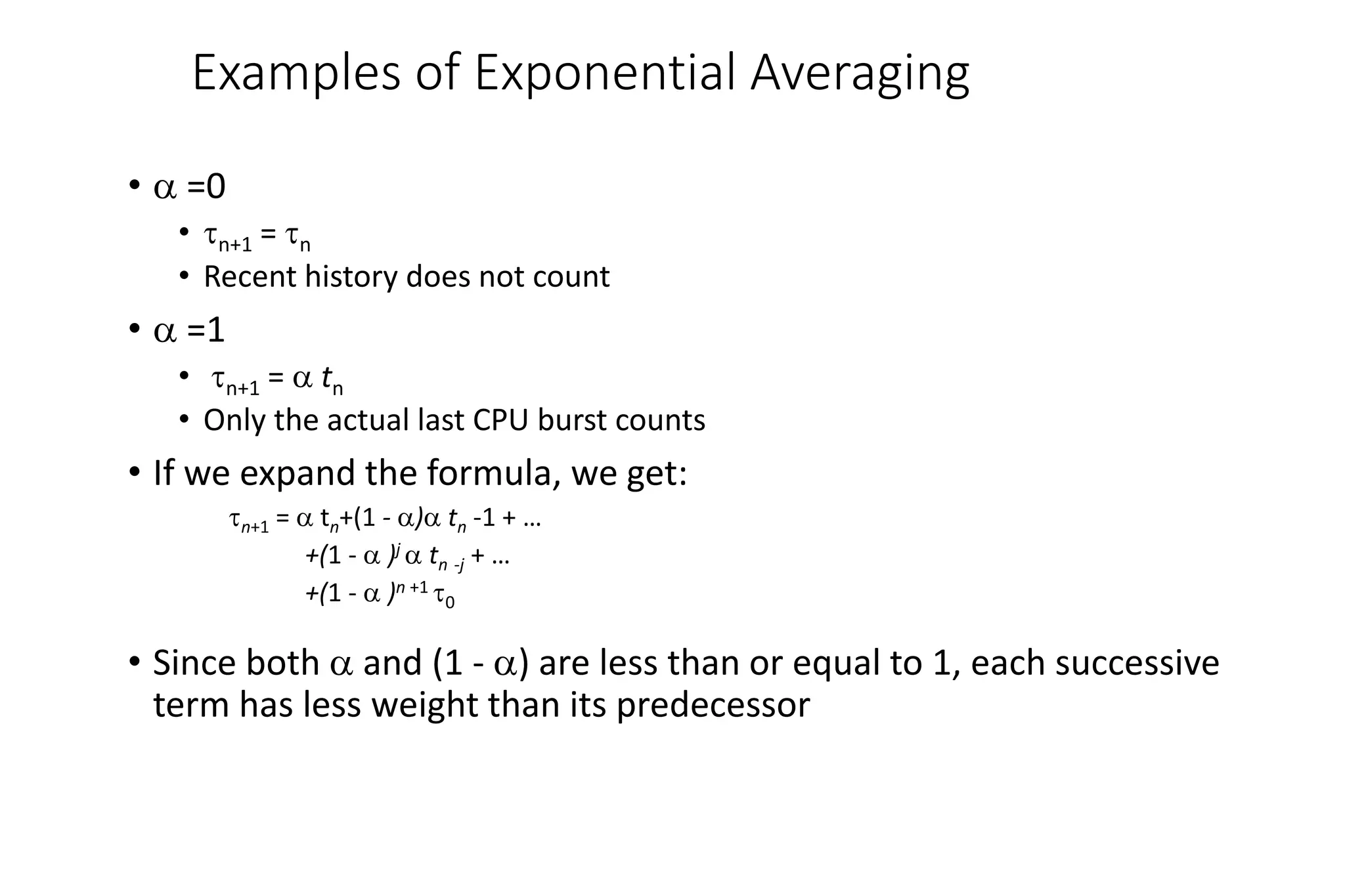
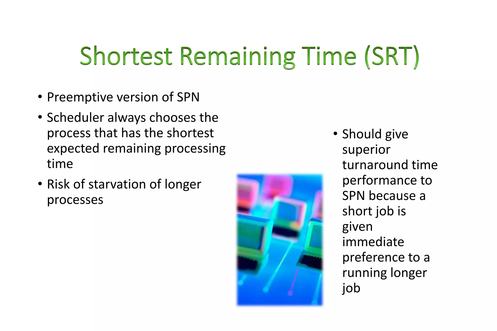
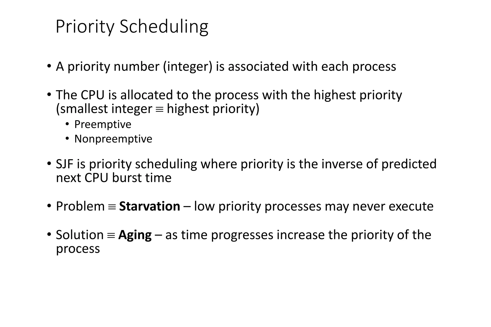
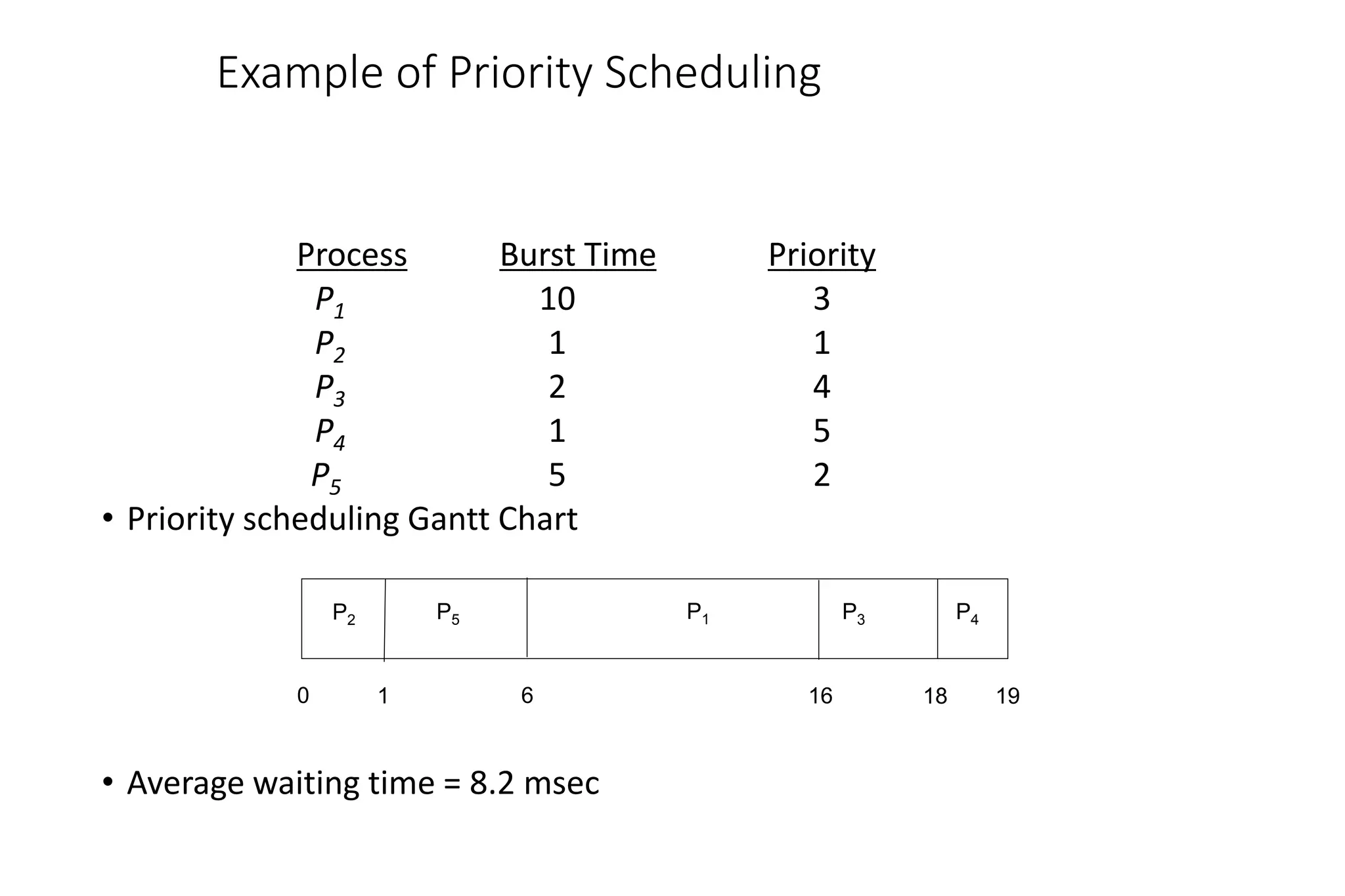
First-come, first-served (FCFS) assigns processes in the order they arrive without preemption. Shortest-job-first (SJF) selects the process with the shortest estimated run time, but may result in starvation of longer processes. Priority scheduling assigns priorities to processes and selects the highest priority process, but low priority processes risk starvation.

![Example of Shortest-remaining-time-first
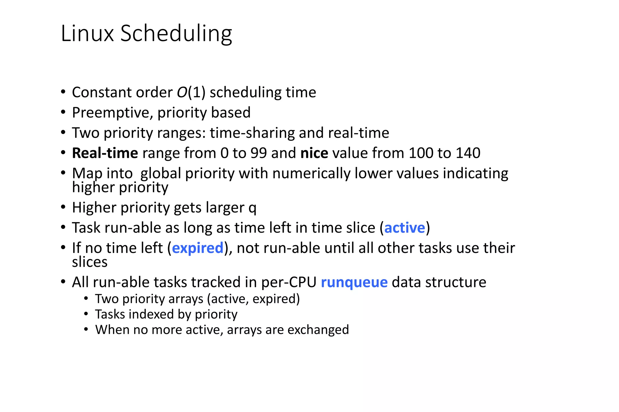
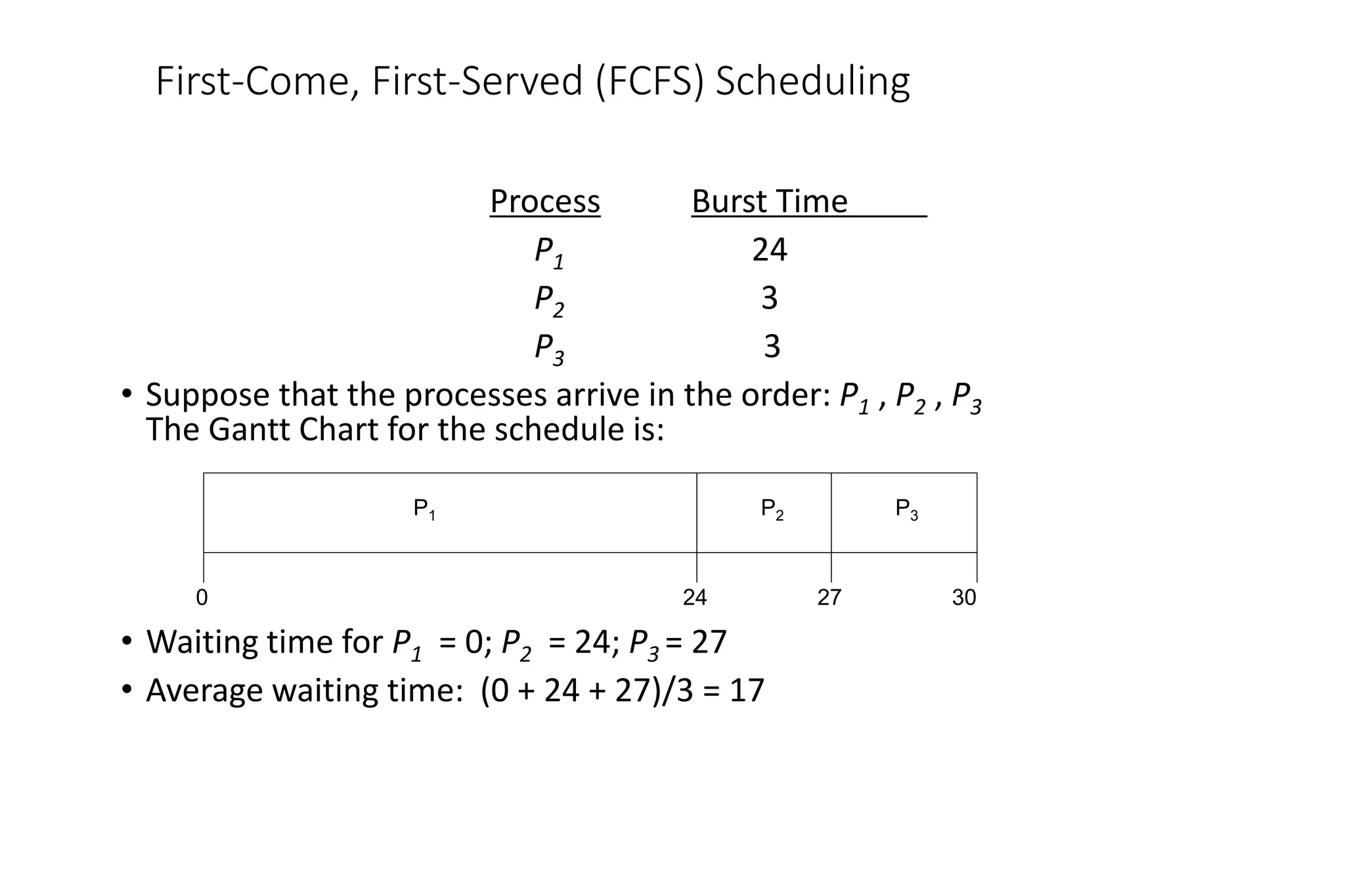
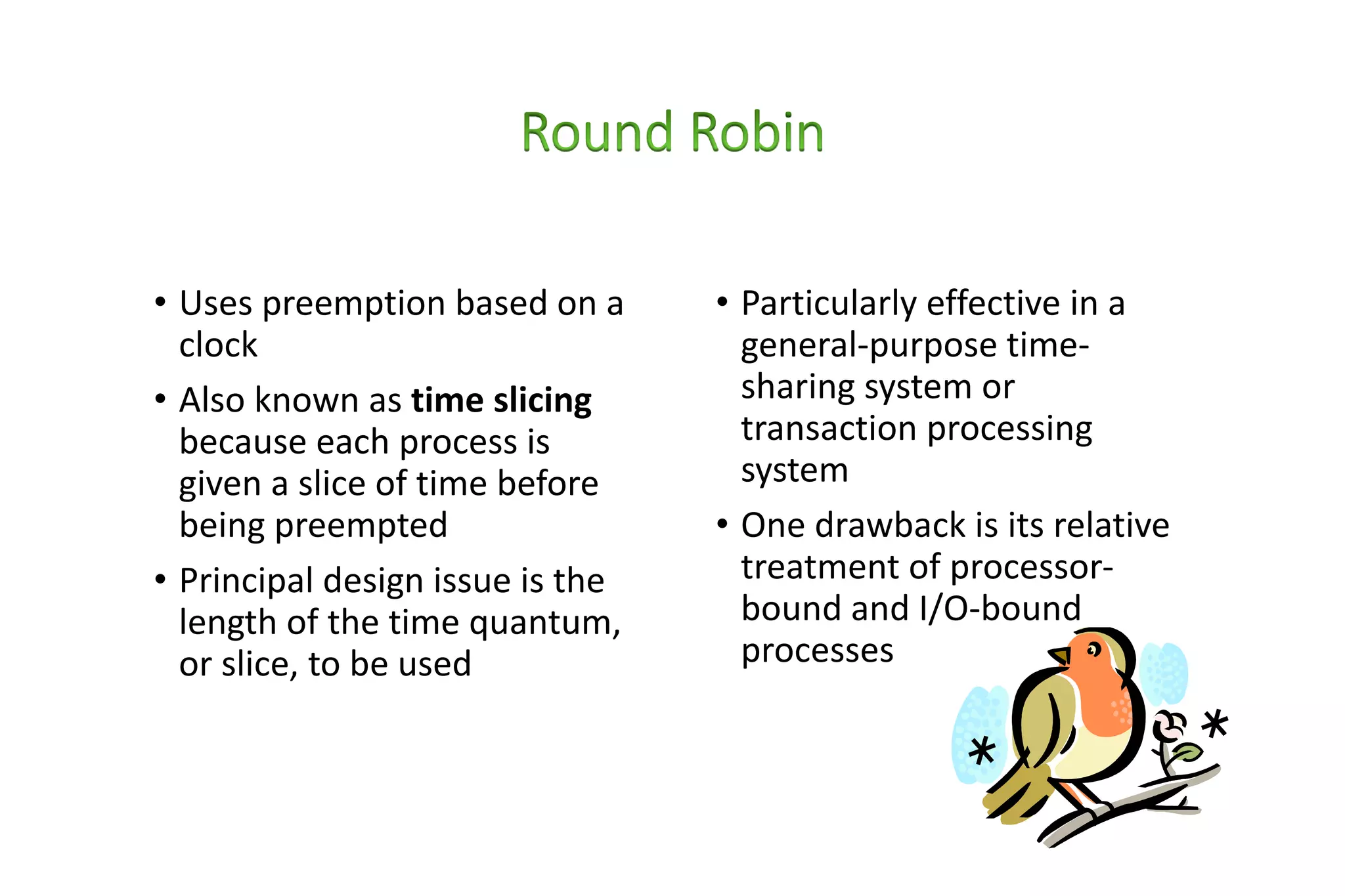
• Now we add the concepts of varying arrival times and preemption to the analysis
ProcessA arri Arrival TimeT Burst Time
P1 0 8
P2 1 4
P3 2 9
P4 3 5
• Preemptive SJF Gantt Chart
• Average waiting time = [(10-1)+(1-1)+(17-2)+5-3)]/4 = 26/4 = 6.5 msec
P1
P1
P2
1 17
0 10
P3
26
5
P4](https://image.slidesharecdn.com/chscheduling1-221215115901-f8d03bc4/75/ch_scheduling-1-ppt-33-2048.jpg)
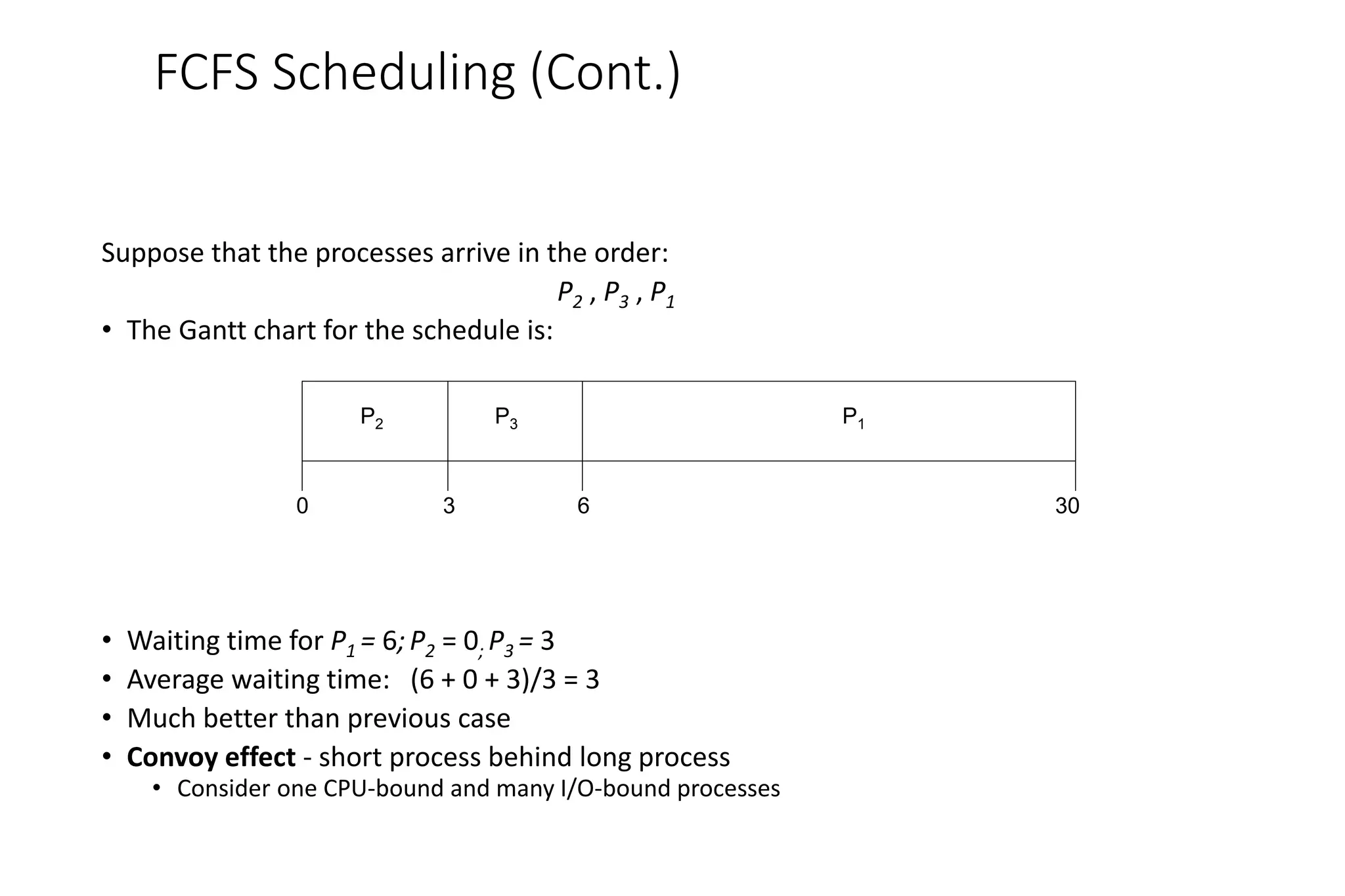
![Pthread Scheduling API
#include <pthread.h>
#include <stdio.h>
#define NUM THREADS 5
int main(int argc, char *argv[])
{
int i;
pthread t tid[NUM THREADS];
pthread attr t attr;
/* get the default attributes */
pthread attr init(&attr);
/* set the scheduling algorithm to PROCESS or SYSTEM */
pthread attr setscope(&attr, PTHREAD SCOPE SYSTEM);
/* set the scheduling policy - FIFO, RT, or OTHER */
pthread attr setschedpolicy(&attr, SCHED OTHER);
/* create the threads */
for (i = 0; i < NUM THREADS; i++)
pthread create(&tid[i],&attr,runner,NULL);](https://image.slidesharecdn.com/chscheduling1-221215115901-f8d03bc4/75/ch_scheduling-1-ppt-48-2048.jpg)
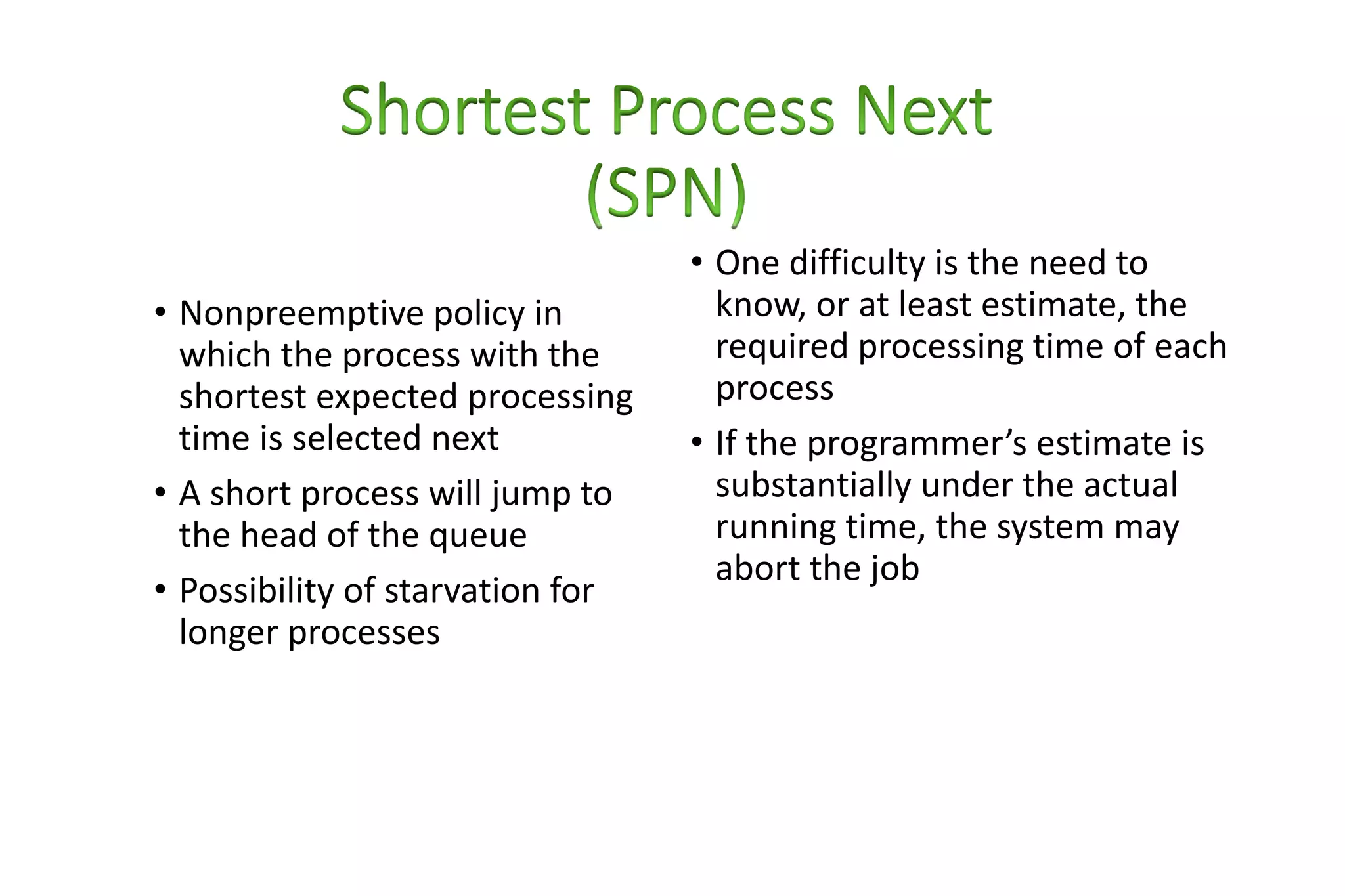
![Pthread Scheduling API
/* now join on each thread */
for (i = 0; i < NUM THREADS; i++)
pthread join(tid[i], NULL);
}
/* Each thread will begin control in this function */
void *runner(void *param)
{
printf("I am a threadn");
pthread exit(0);
}](https://image.slidesharecdn.com/chscheduling1-221215115901-f8d03bc4/75/ch_scheduling-1-ppt-49-2048.jpg)