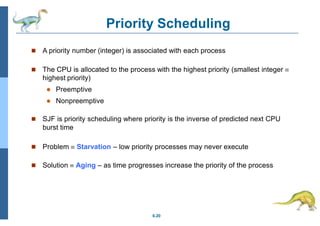
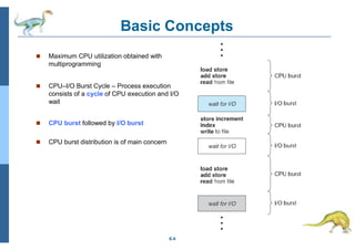
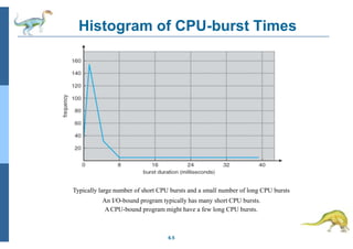
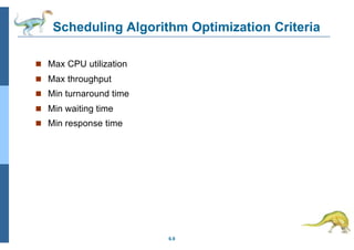
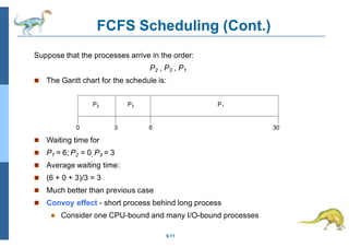
Chapter 5 discusses process scheduling, introducing key concepts, scheduling criteria, and various algorithms, such as First-Come, First-Served, Shortest Job First, and Round Robin. The document emphasizes the importance of CPU utilization, throughput, and turnaround time in evaluating scheduling algorithms. It also explores different scheduling methods, including multilevel queues and feedback queues, to optimize CPU allocation for processes.

1. Chapter 5: Process
Scheduling
C. P. Divate

2. Chapter 5: Process Scheduling
6.2
 Basic Concepts
 Scheduling Criteria
 Scheduling Algorithms
 Thread Scheduling
 Multiple-Processor Scheduling
 Real-Time CPU Scheduling
 Operating Systems Examples
 Algorithm Evaluation

3. Objectives
6.3
 To introduce CPU scheduling, which is the basis for multiprogrammed operating
systems
 To describe various CPU-scheduling algorithms
 To discuss evaluation criteria for selecting a CPU-scheduling algorithm for a
particular system
 To examine the scheduling algorithms of several operating systems

4. Basic Concepts
 Maximum CPU utilization obtained with
multiprogramming
 CPU–I/O Burst Cycle – Process execution
consists of a cycle of CPU execution and I/O
wait
 CPU burst followed by I/O burst
 CPU burst distribution is of main concern
6.4

5. Histogram of CPU-burst Times
Typically large number of short CPU bursts and a small number of long CPU bursts
An I/O-bound program typically has many short CPU bursts.
ACPU-bound program might have a few long CPU bursts.
6.5

6. CPU Scheduler
6.6
 Short-term scheduler selects from among the processes in ready queue, and
allocates the CPU to one of them
 Queue may be ordered in various ways
 CPU scheduling decisions may take place when a process:
1. Switches from running to waiting state
2. Switches from running to ready state
3. Switches from waiting to ready
4. Terminates
 Scheduling under 1 and 4 is nonpreemptive
 All other scheduling is preemptive
 Consider access to shared data
 Consider preemption while in kernel mode
 Consider interrupts occurring during crucial OS activities

7. Dispatcher
6.7
 Dispatcher module gives control of the CPU to the process selected by the
short-term scheduler; this involves:
 switching context
 switching to user mode
 jumping to the proper location in the user program to restart that program
 Dispatch latency – time it takes for the dispatcher to stop one process and start
another running

8. Scheduling Criteria
6.8
 CPU utilization – keep the CPU as busy as possible
 Throughput – # of processes that complete their execution per time unit
 Turnaround time – amount of time to execute a particular process
 Waiting time – amount of time a process has been waiting in the ready queue
 Response time – amount of time it takes from when a request was submitted
until the first response is produced, not output (for time-sharing environment)

9. Scheduling Algorithm Optimization Criteria
6.9
 Max CPU utilization
 Max throughput
 Min turnaround time
 Min waiting time
 Min response time

10. First-Come, First-Served (FCFS) Scheduling
Process Burst Time
P1 24
P2 3
P3 3
 Suppose that the processes arrive in the order: P1 , P2 , P3
The Gantt Chart for the schedule is:
P1 P2 P3
24
6.10
27 30
0
 Waiting time for
 P1 = 0; P2 = 24; P3 = 27
 Average waiting time:
 (0 + 24 + 27)/3 = 17

11. FCFS Scheduling (Cont.)
Suppose that the processes arrive in the order:
P2 , P3 , P1
 The Gantt chart for the schedule is:
 P1 = 6; P2 = 0; P3 = 3
 Average waiting time:
 (6 + 0 + 3)/3 = 3
 Much better than previous case
 Convoy effect - short process behind long process
 Consider one CPU-bound and many I/O-bound processes
P1
P3
P2
6
6.11
3 30
0
 Waiting time for

12. Shortest-Job-First (SJF) Scheduling
6.12
 Associate with each process the length of its next CPU burst
 Use these lengths to schedule the process with the shortest time
 SJF is optimal – gives minimum average waiting time for a given set of
processes
 The difficulty is knowing the length of the next CPU request
 Could ask the user

13. Example of SJF
Process Burst Time
P1 6
P2 8
P3 7
P4 3
 SJF scheduling chart
 Average waiting time =
 (3 + 16 + 9 + 0) / 4 = 7
P4 P3
P1
3 16
0 9
P2
6.13
24

14. Determining Length of Next CPU Burst
6.14
 Can only estimate the length – should be similar to the previous one
 Then pick process with shortest predicted next CPU burst
 Can be done by using the length of previous CPU bursts, using exponential
averaging
1. tn  actual length of nth
CPU burst
2. n 1  predicted value for the next CPU burst
3. , 0    1
 Commonly, αset to ½
 Preemptive version called shortest-remaining-time-first
4. Define :    t  1    .
n 1 n n

15. Prediction of the Length of the
Next CPU Burst
6.15

16. Examples of Exponential Averaging
6.16
  =0
 n+1 = n
 Recent history does not count
  =1
 n+1 =  tn
 Only the actual last CPU burst counts
 If we expand the formula, we get:
n+1 =  tn+(1 - ) tn -1 + …
+(1 -  )j  tn -j + …
+(1 -  )n +1 0
 Since both  and (1 - ) are less than or equal to 1, each successive term has
less weight than its predecessor

17. Example of Shortest-remaining-time-first
 Now we add the concepts of varying arrival times and preemption to the analysis
Process Arrival Time Burst Time
P1 0 8
P2 1 4
P3 2 9
P4 3 5
0 1 5 10 17 26
 Average waiting time = [(10-1)+(1-1)+(17-2)+5-3)]/4 = 26/4 = 6.5 msec
P1 P3
6.17
 Preemptive SJF Gantt Chart
P1 P2 P4

18. Diagram of Process State
3.18

19. Representation of Process Scheduling
● Queueing diagram represents queues, resources, flows
3.19

20. Priority Scheduling
6.20
 A priority number (integer) is associated with each process
 The CPU is allocated to the process with the highest priority (smallest integer 
highest priority)
 Preemptive
 Nonpreemptive
 SJF is priority scheduling where priority is the inverse of predicted next CPU
burst time
 Problem  Starvation – low priority processes may never execute
 Solution  Aging – as time progresses increase the priority of the process

21. Example of Priority Scheduling
Process Burst Time Priority
P1 10 3
P2 1 1
P3 2 4
P4 1 5
P5 5 2
 Priority scheduling Gantt Chart
0 1
 Average waiting time =
8.2 msec
P2 P3
P5
18 19
6.21
16
P4
6
P1

22. Round Robin (RR)
6.22
 Each process gets a small unit of CPU time (time quantum q), usually 10-100
milliseconds. After this time has elapsed, the process is preempted and added
to the end of the ready queue.
 If there are n processes in the ready queue and the time quantum is q, then
each process gets 1/n of the CPU time in chunks of at most q time units at
once. No process waits more than (n-1)q time units.
 Timer interrupts every quantum to schedule next process
 Performance
 q large  FIFO
 q small  q must be large with respect to context switch, otherwise
overhead is too high

23. Example of RR with Time Quantum = 4
Process Burst Time
P1 24
P2 3
P3 3
 The Gantt chart is:
0 4 7 10 14 18 22 26 30
 Typically, higher average turnaround than SJF, but better response
 q should be large compared to context switch time
 q usually 10ms to 100ms, context switch < 10 usec
P1 P2 P3 P1 P1 P1 P1 P1
6.23

24. Time Quantum and Context Switch Time
6.24

25. Turnaround Time Varies With
The Time Quantum
80% of CPU bursts should
be shorter than q
6.25

26. Multilevel Queue
6.26
 Ready queue is partitioned into separate queues, eg:
 foreground (interactive)
 background (batch)
 Process permanently in a given queue
 Each queue has its own scheduling algorithm:
 foreground – RR
 background – FCFS
 Scheduling must be done between the queues:
 Fixed priority scheduling; (i.e., serve all from foreground then from
background). Possibility of starvation.
 Time slice – each queue gets a certain amount of CPU time which it can
schedule amongst its processes;
 i.e., 80% to foreground in RR, 20% to background in FCFS

27. Multilevel Queue Scheduling
6.27

28. Multilevel Feedback Queue
6.28
 A process can move between the various queues; aging can be
implemented this way
 Multilevel-feedback-queue scheduler defined by the following parameters:
 number of queues
 scheduling algorithms for each queue
 method used to determine when to upgrade a process
 method used to determine when to demote a process
 method used to determine which queue a process will enter when that
process needs service