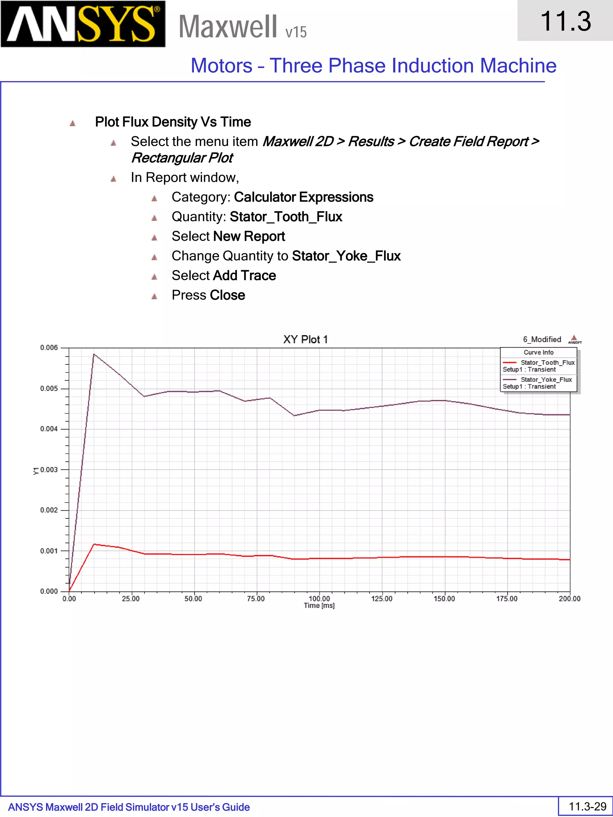
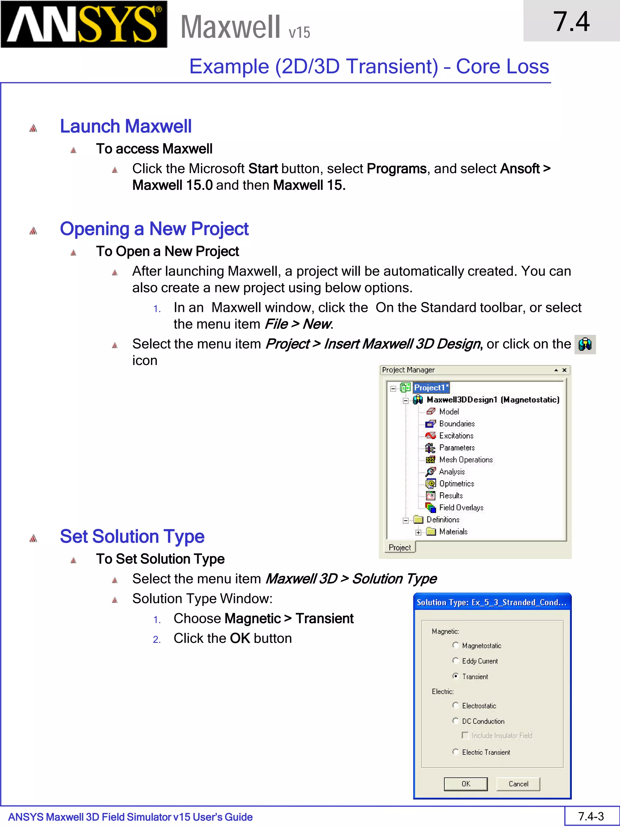
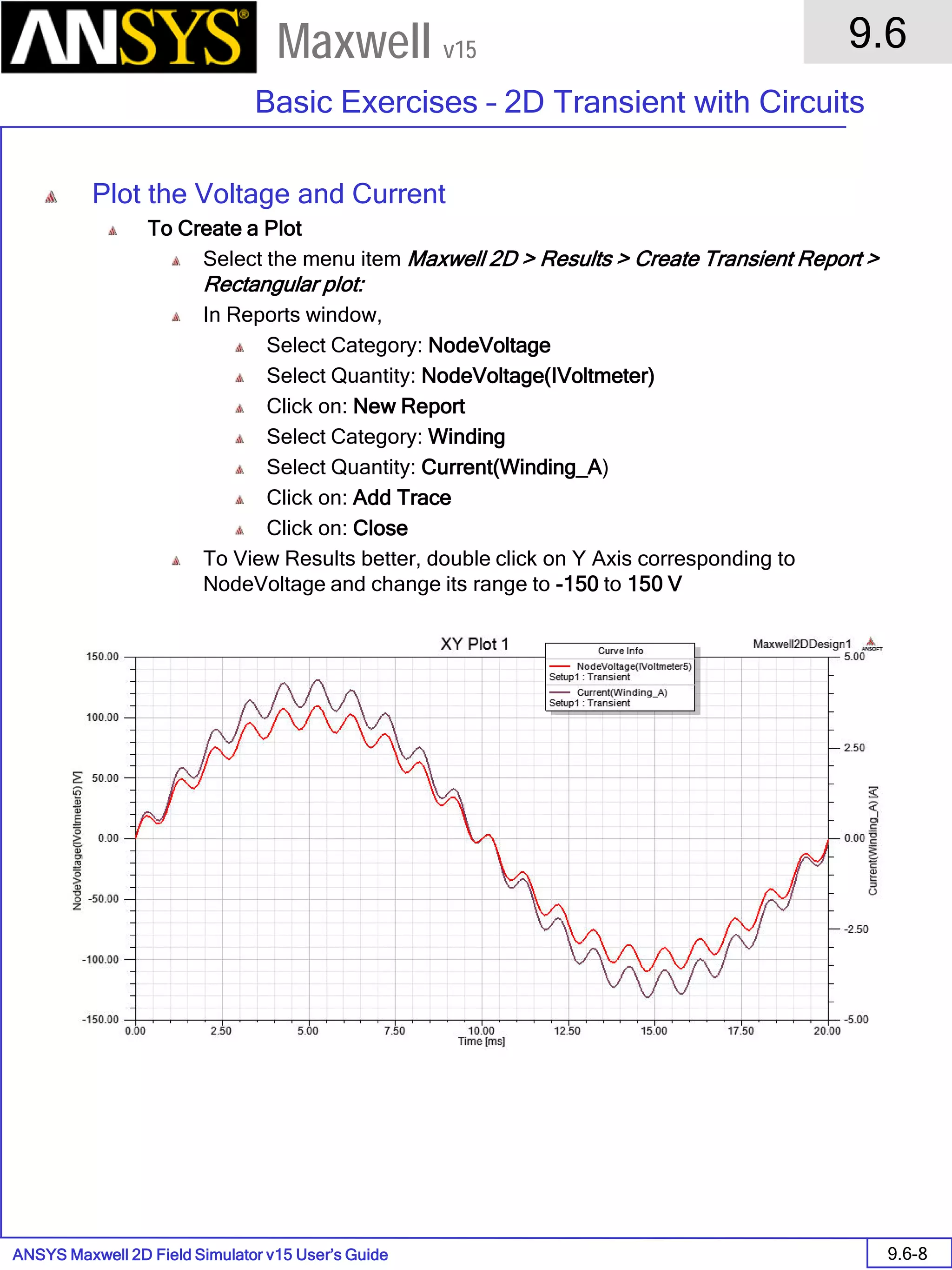
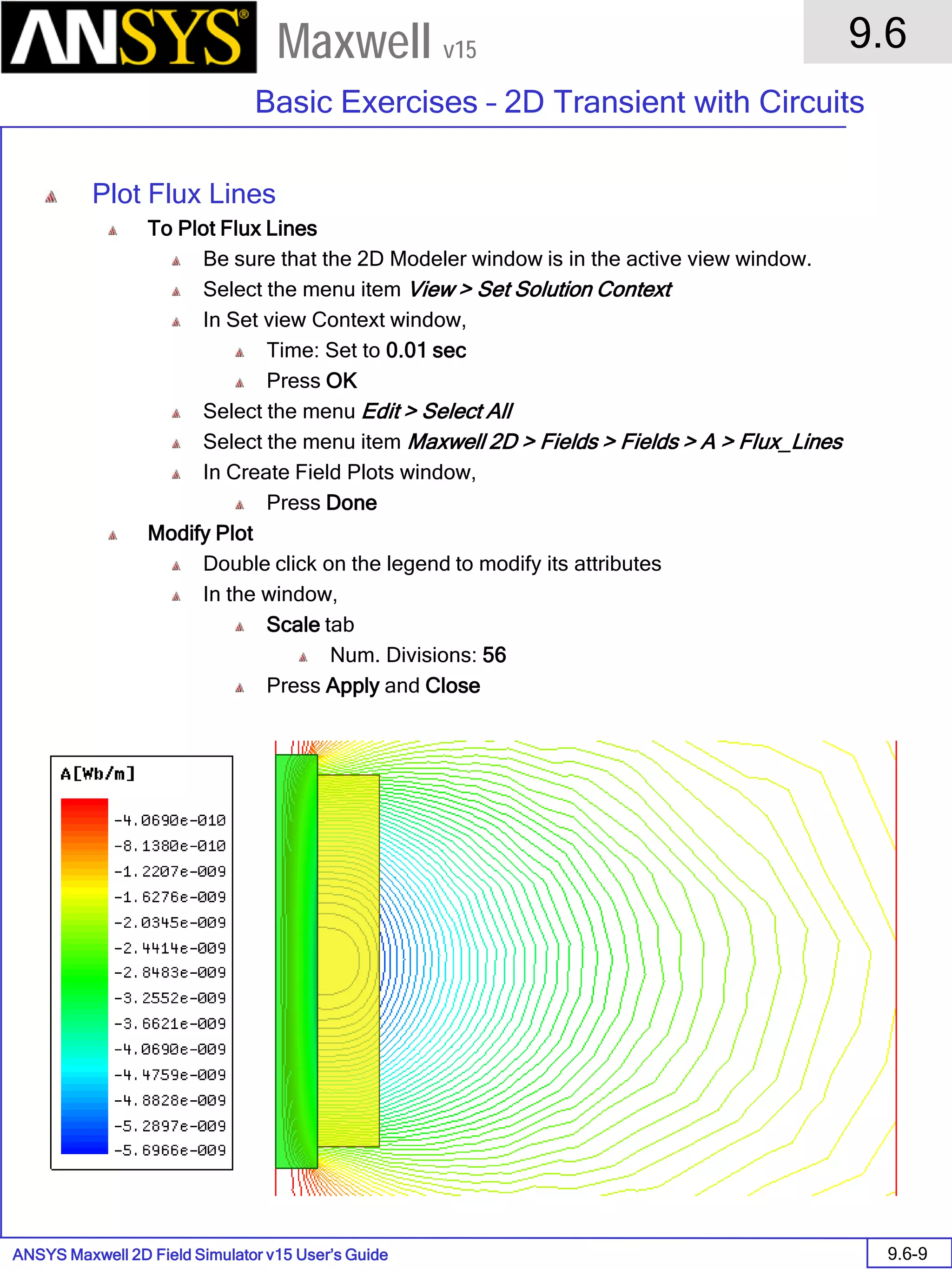
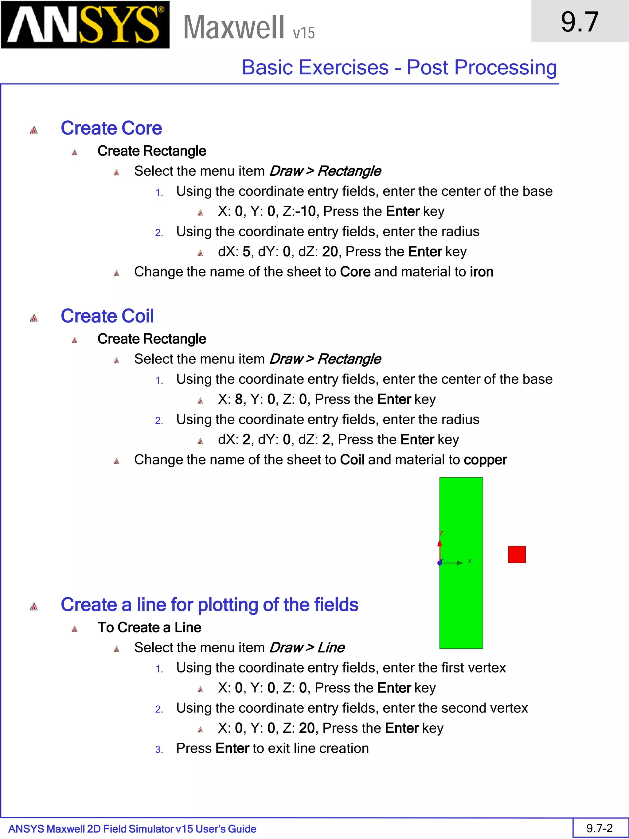
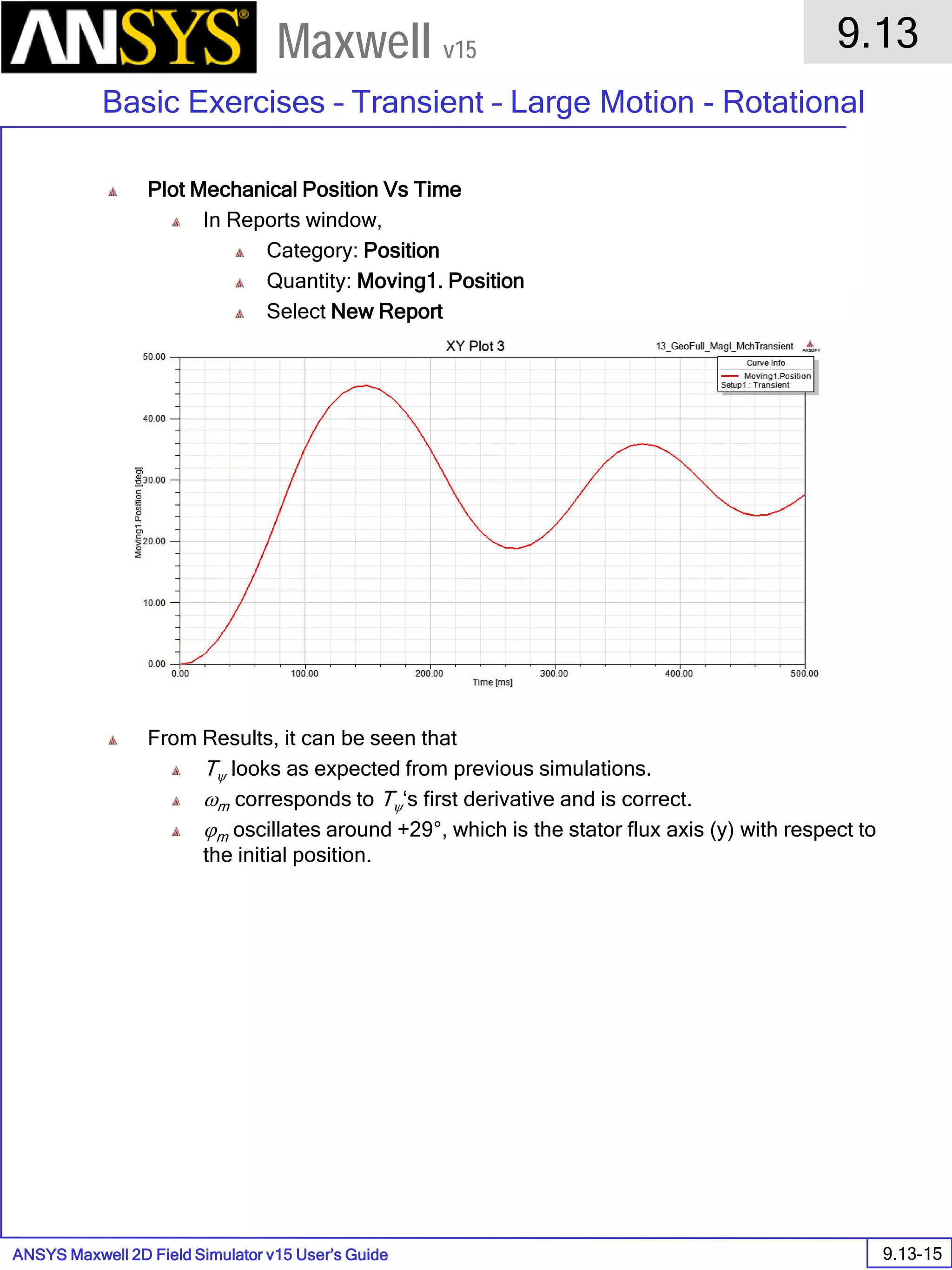
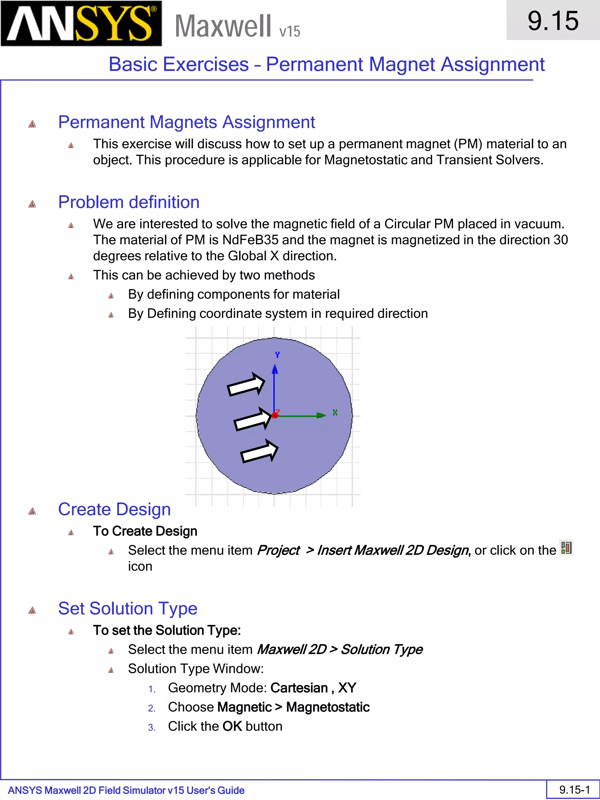
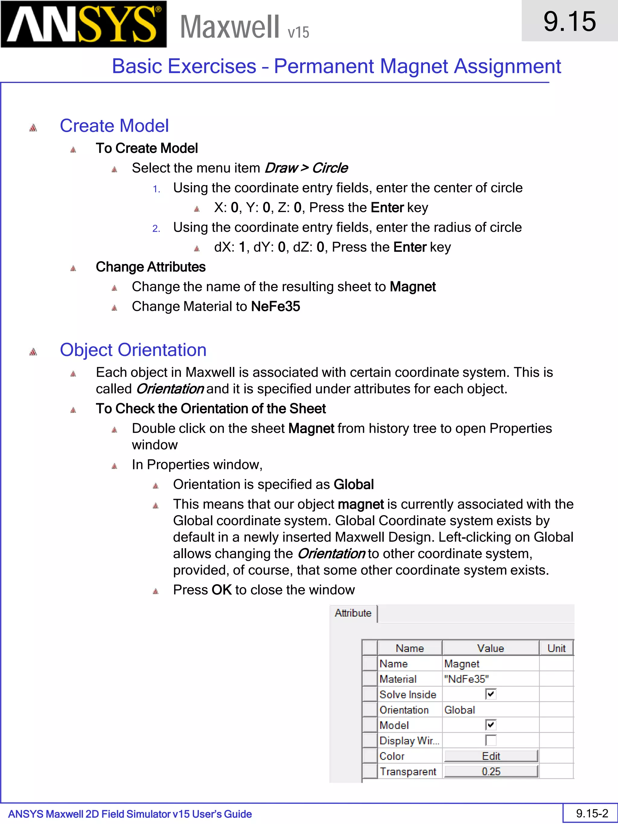
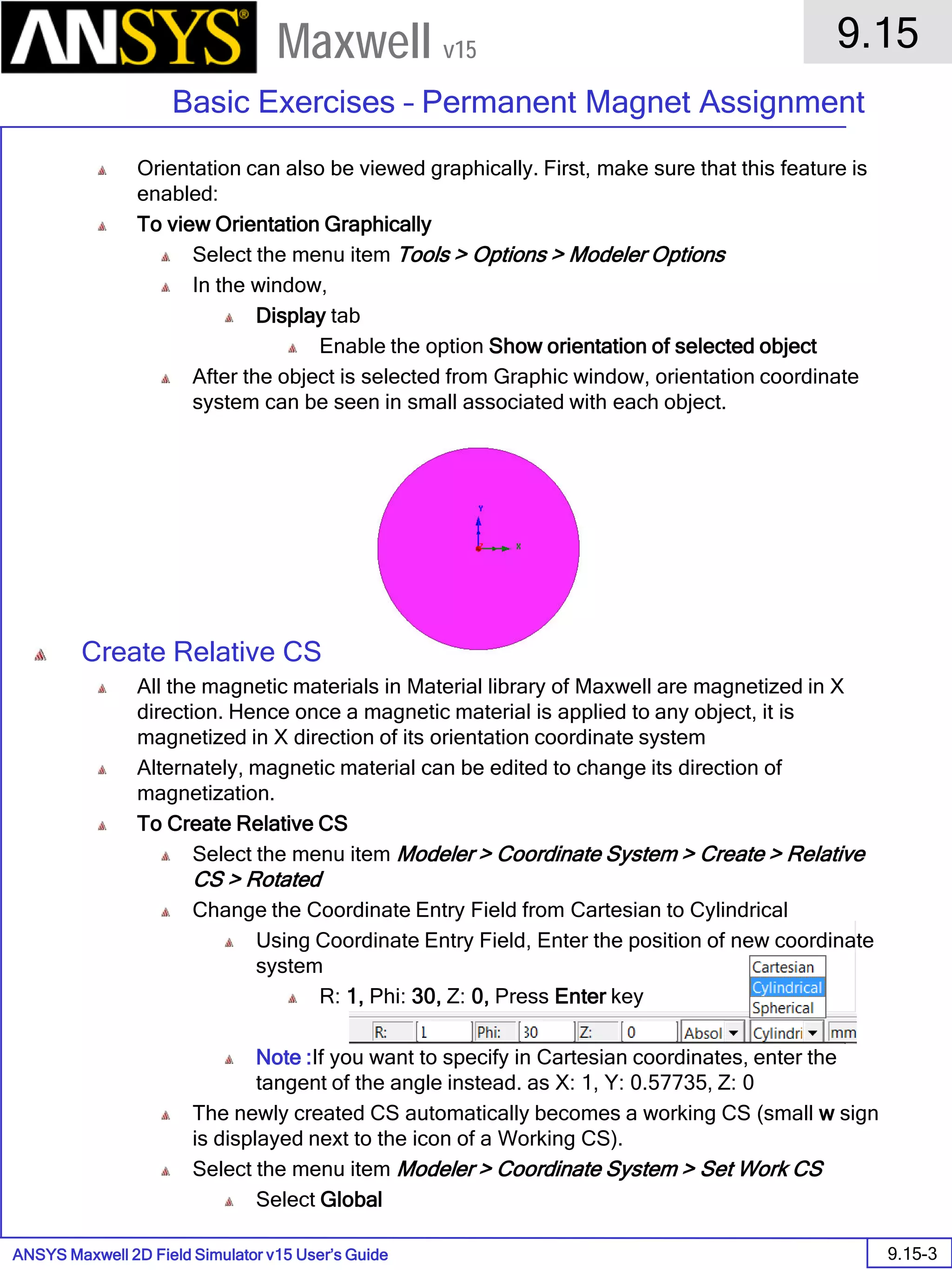
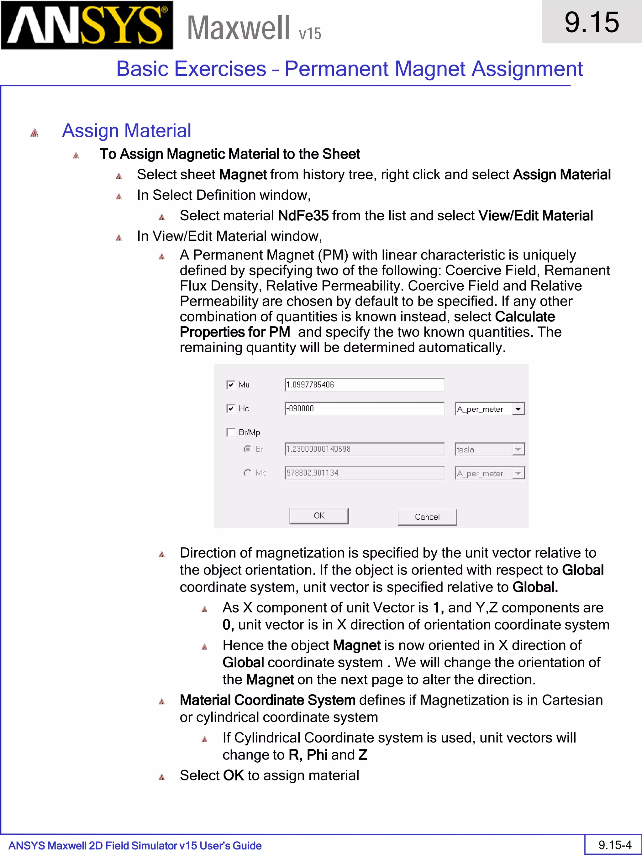
The document is a user's guide for ANSYS Maxwell 2D, a software platform used for electromagnetic and electromechanical analysis via finite element analysis. It outlines the software's capabilities, including various analysis types, drawing geometry, meshing, and solver functionalities, while also providing details about its interface and supported platforms. Additionally, it offers information about project management, solution types, and attributes related to modeling within the software.
![ANSYS Maxwell Field Simulator v15 – Training Seminar P1-8
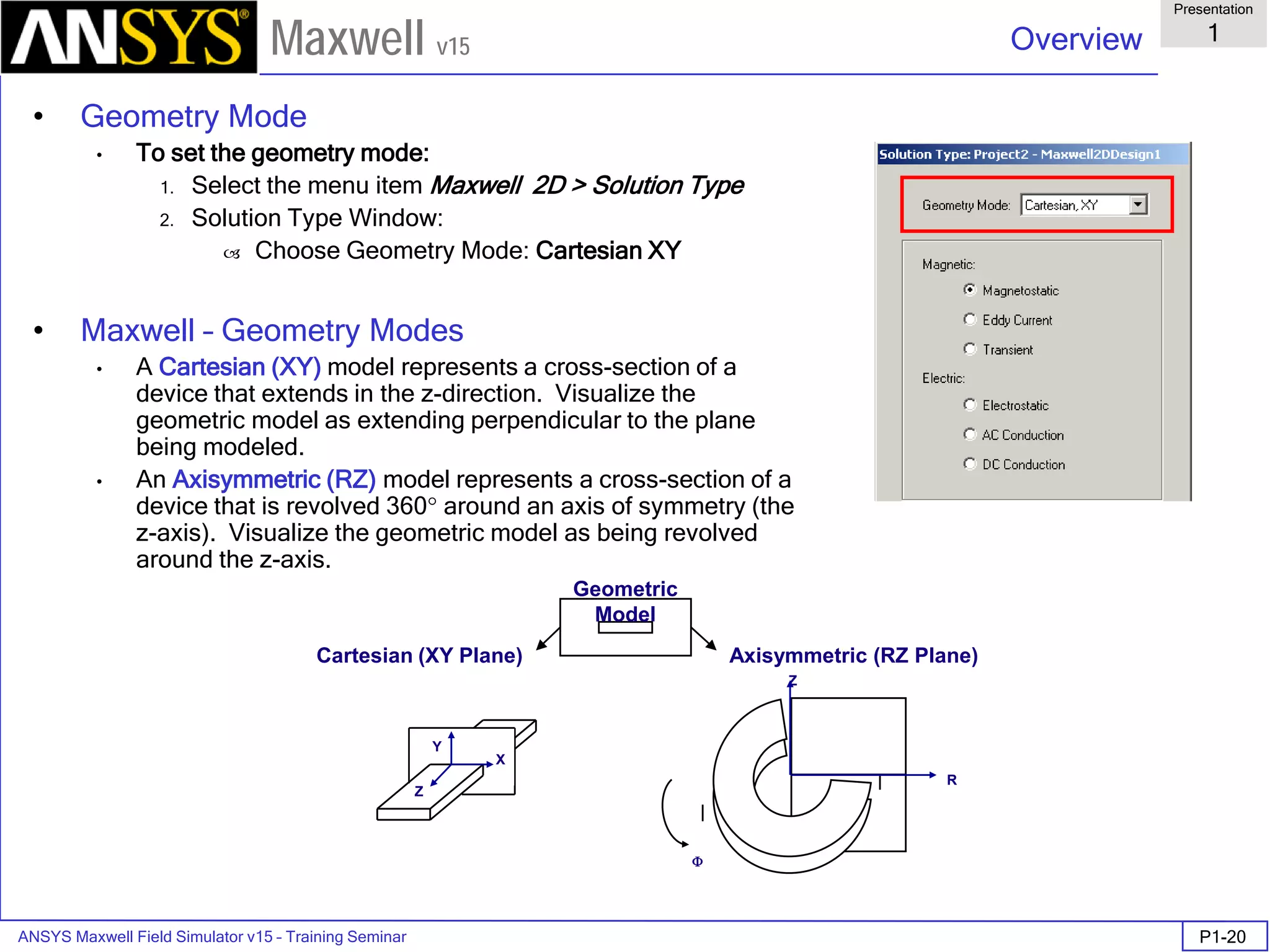
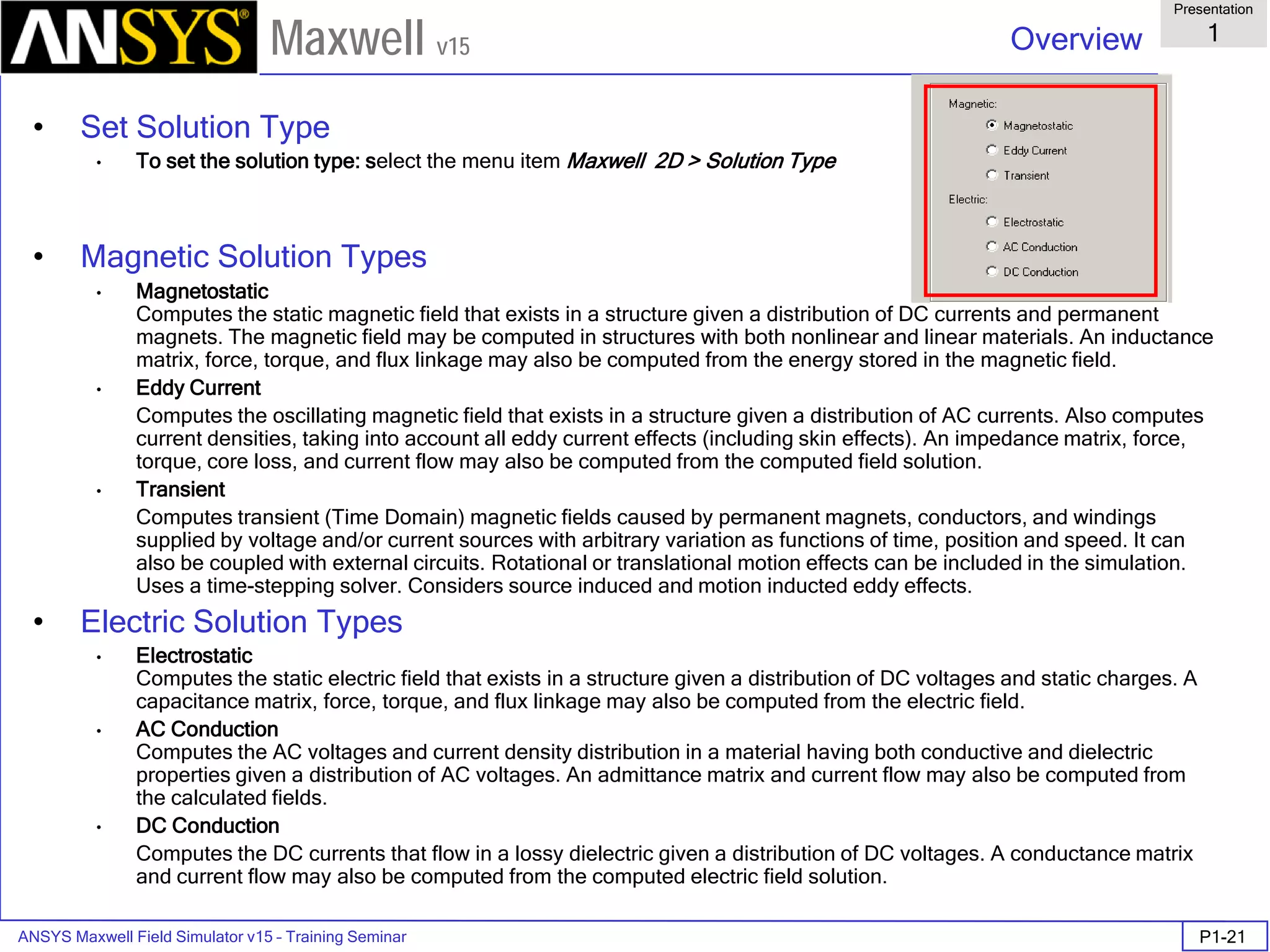
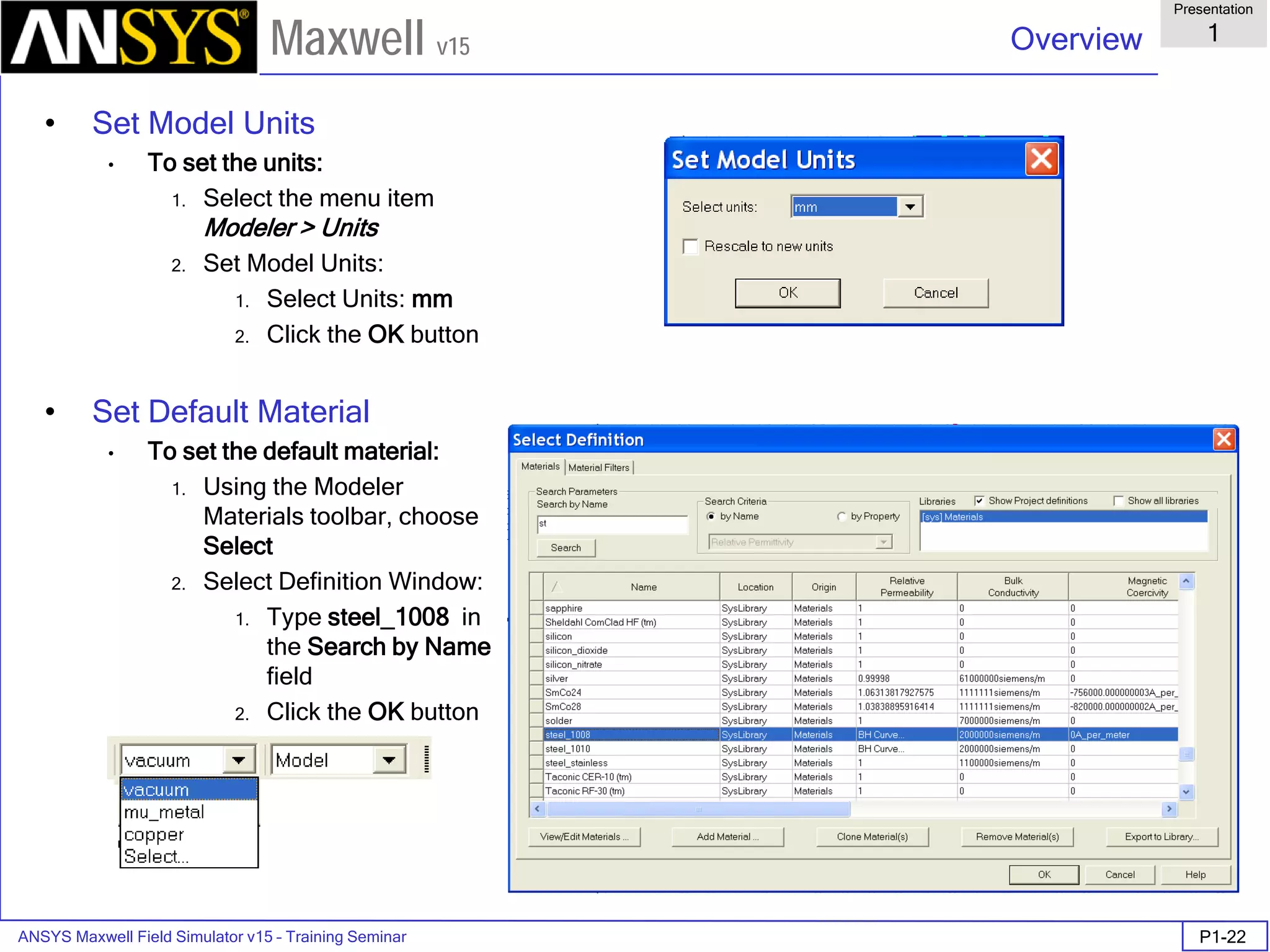
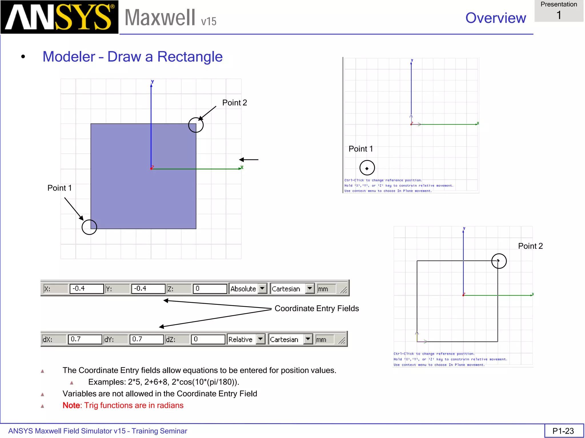
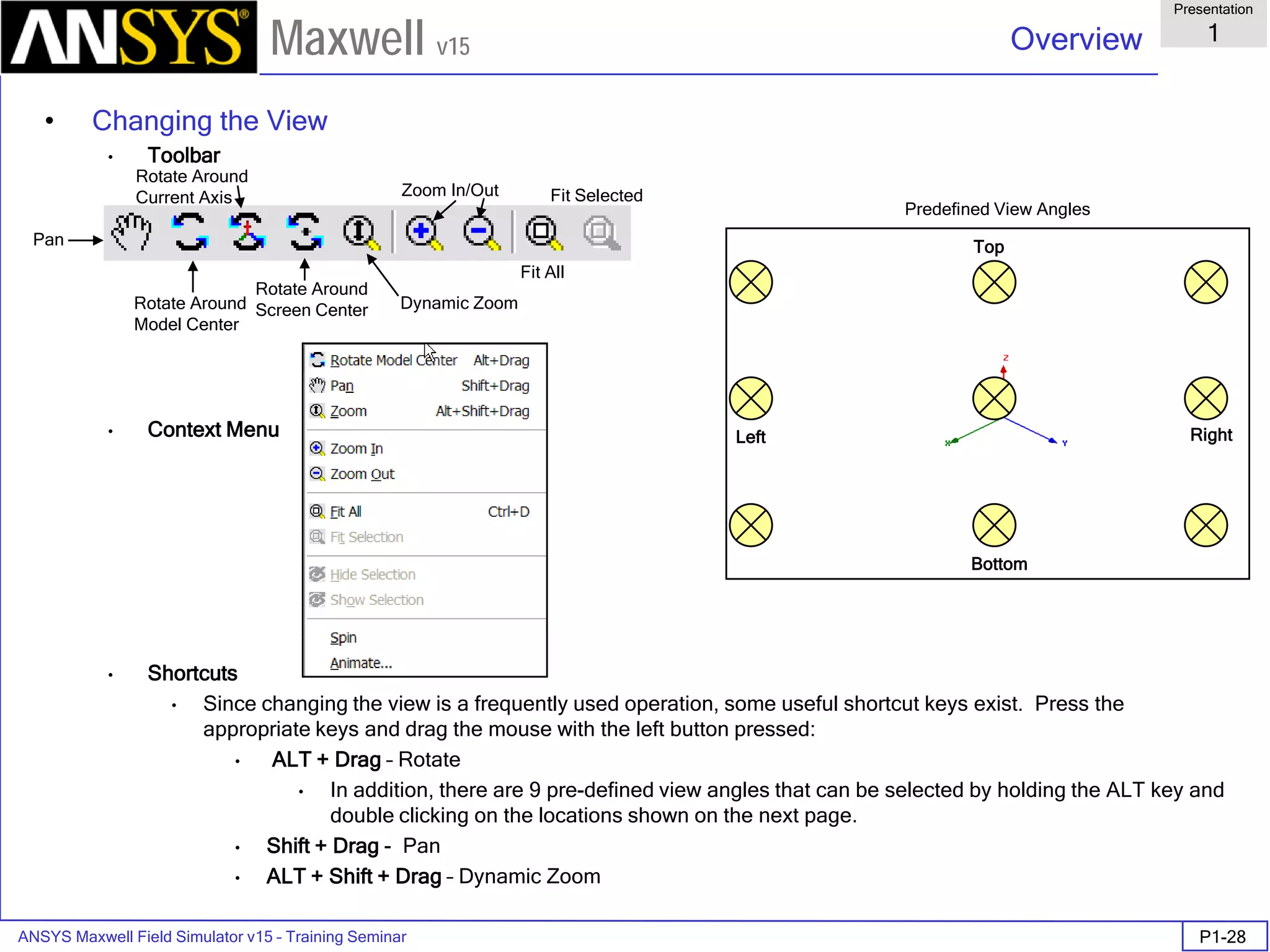
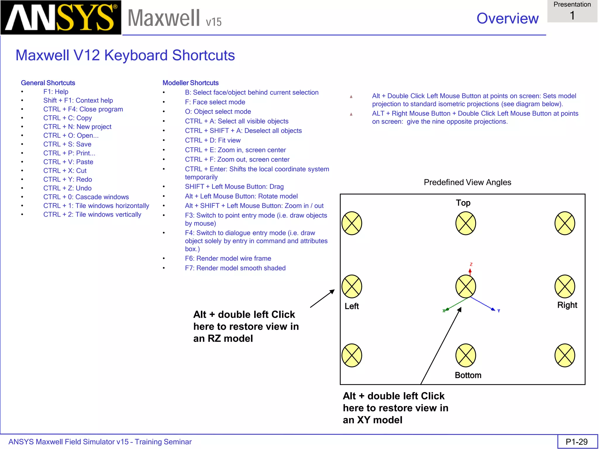
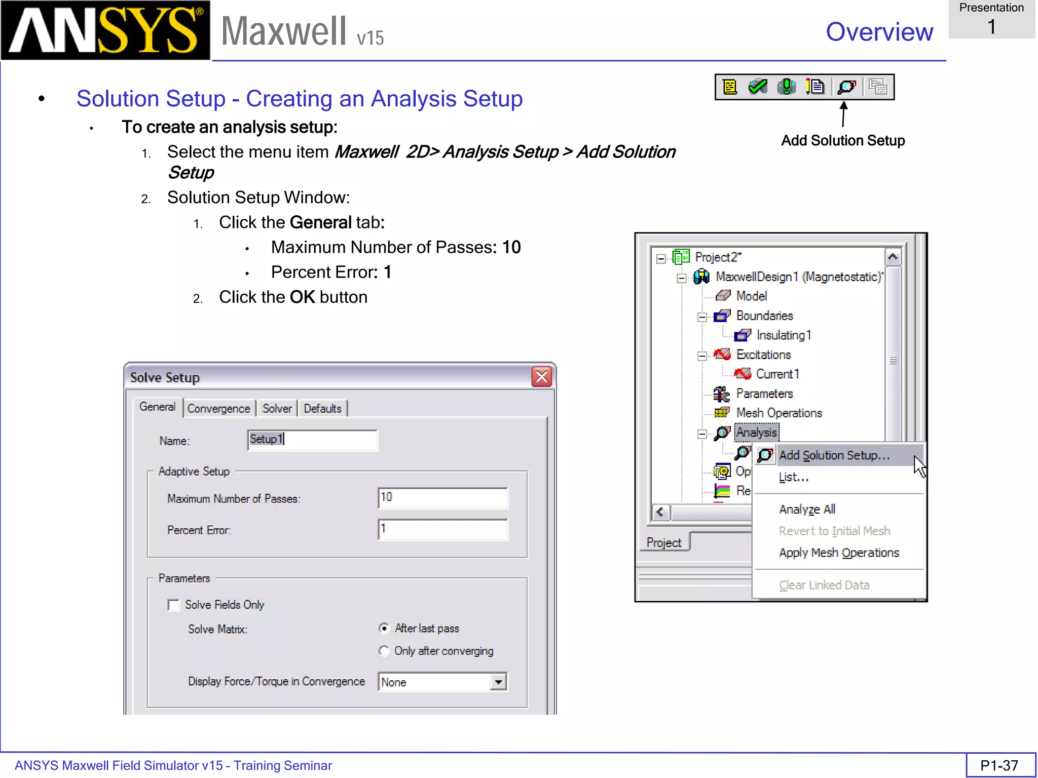
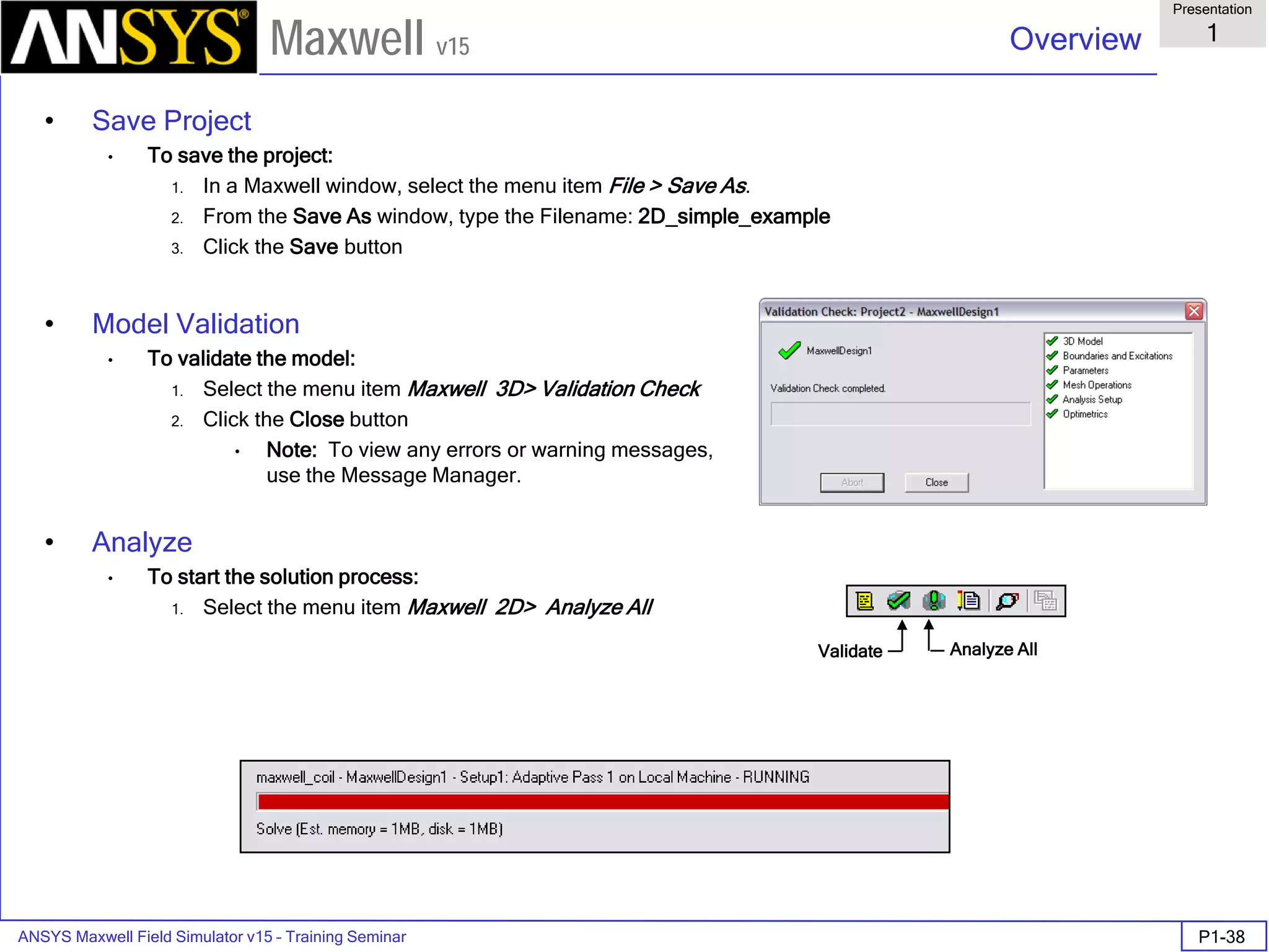
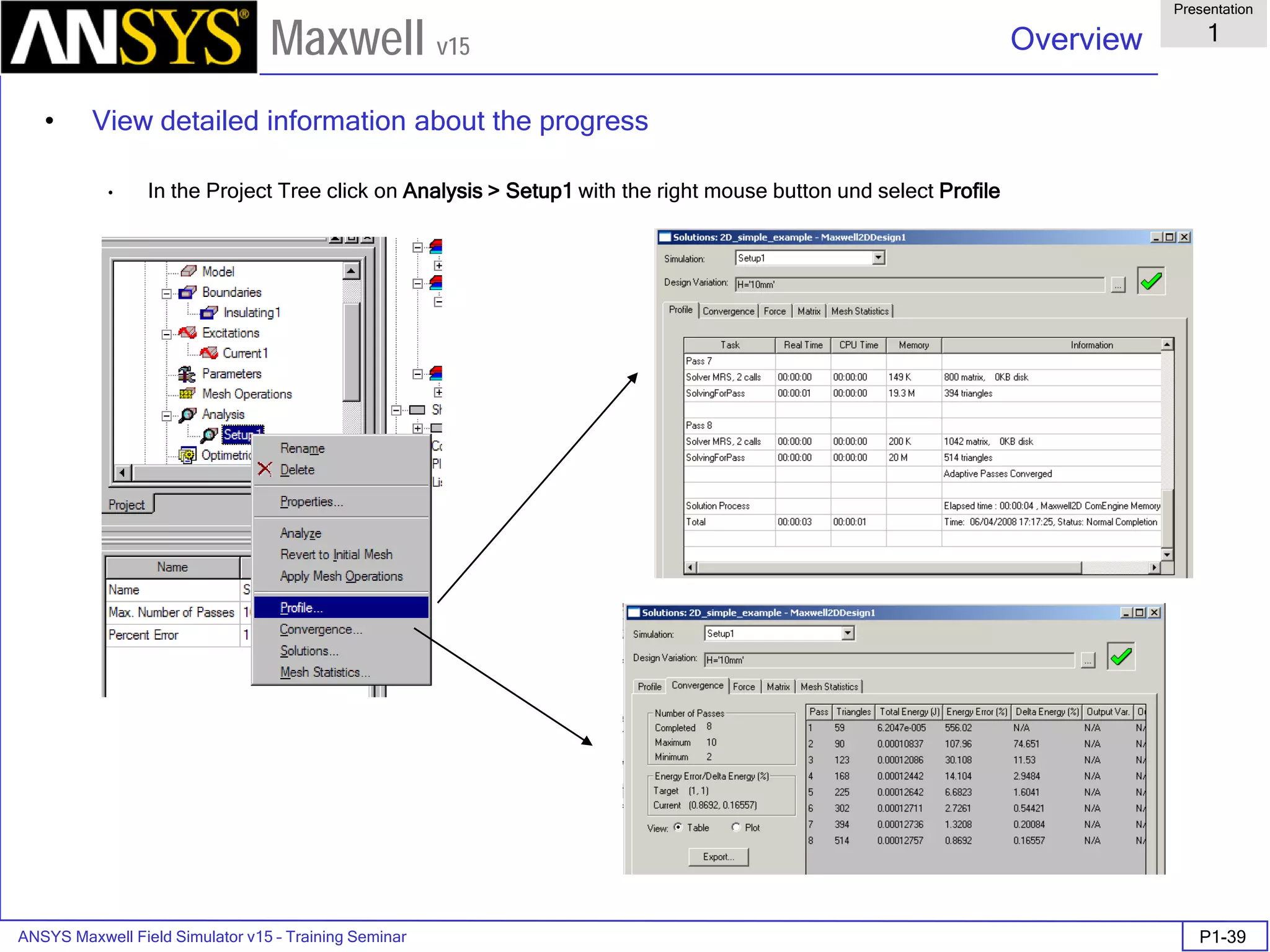
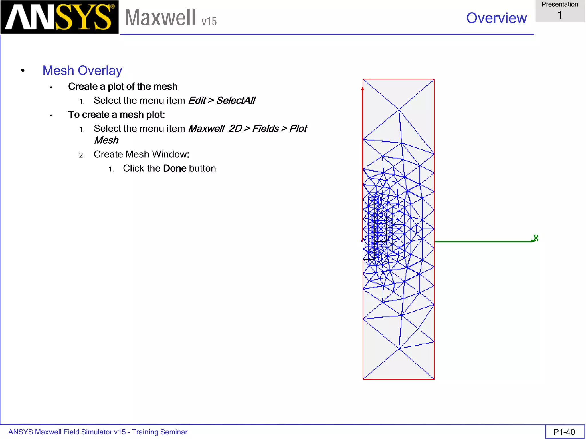
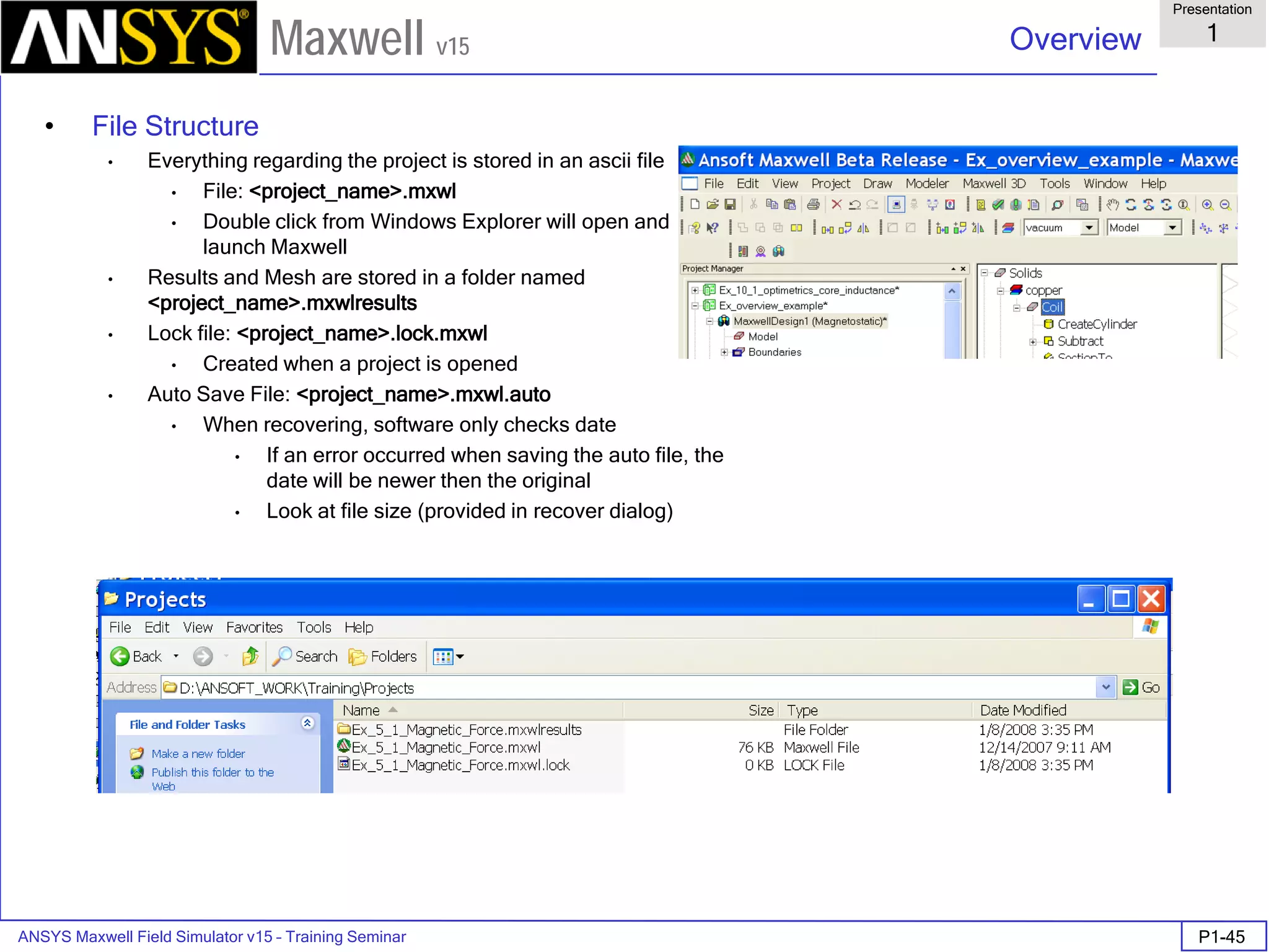
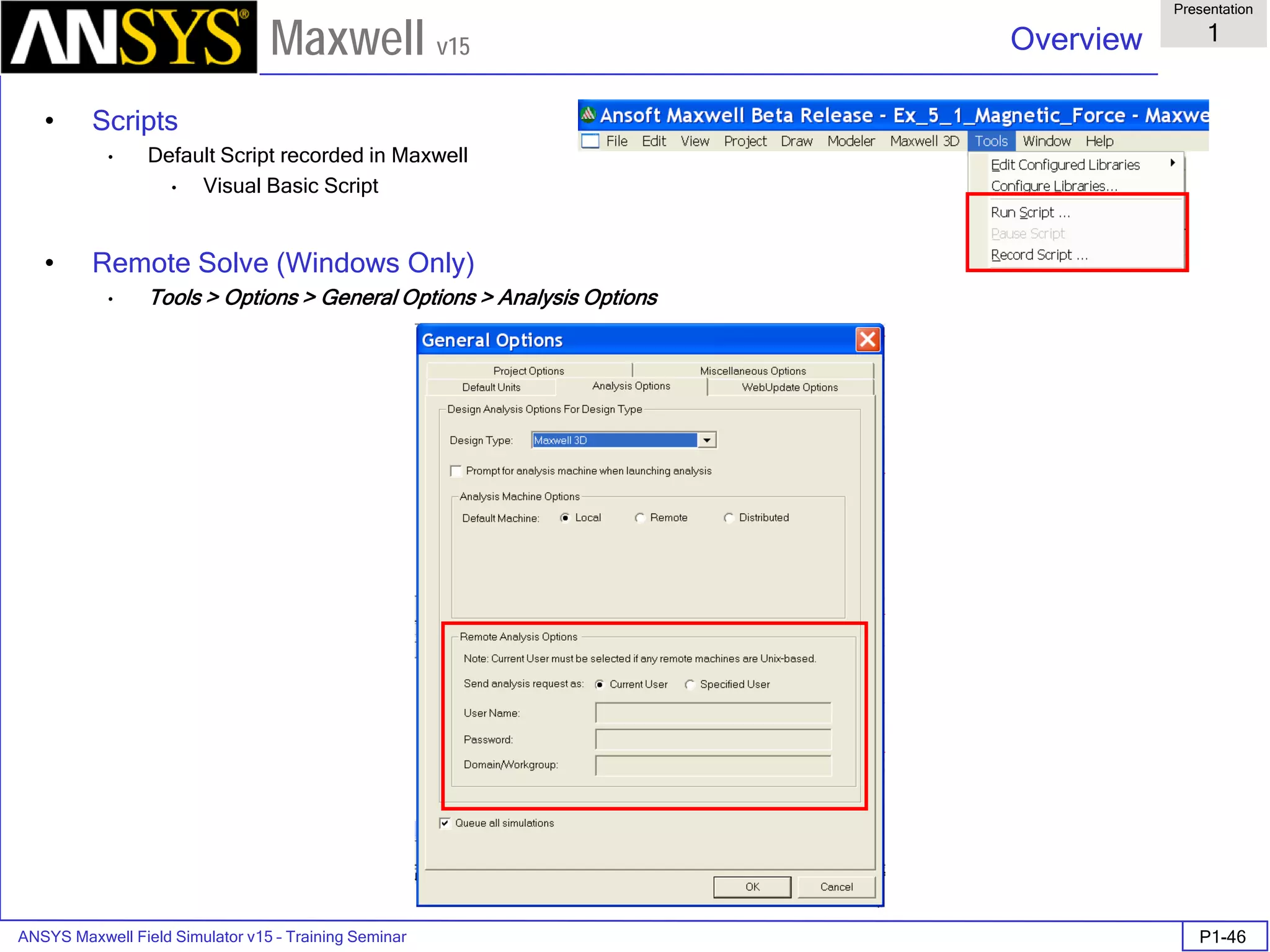
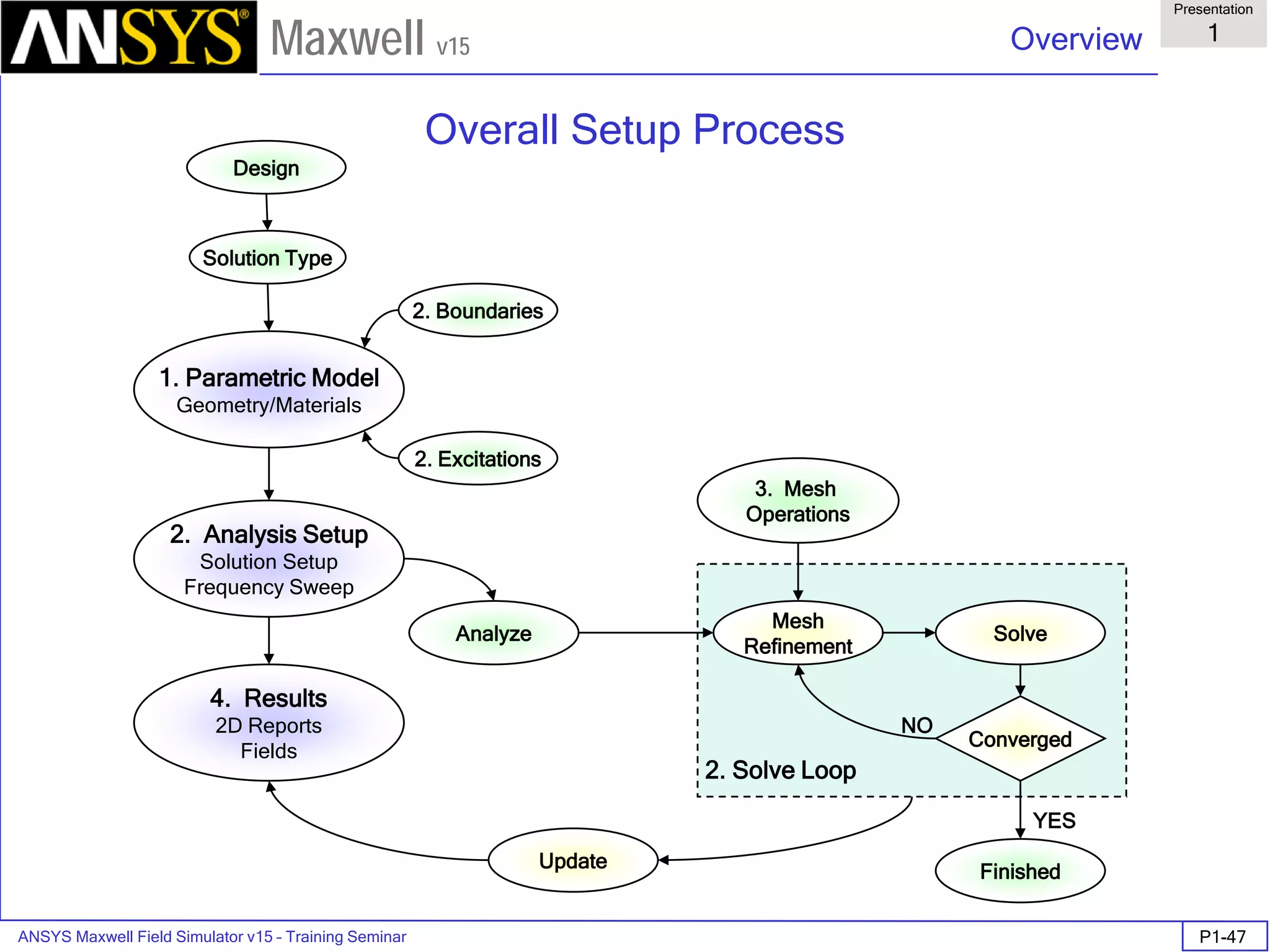
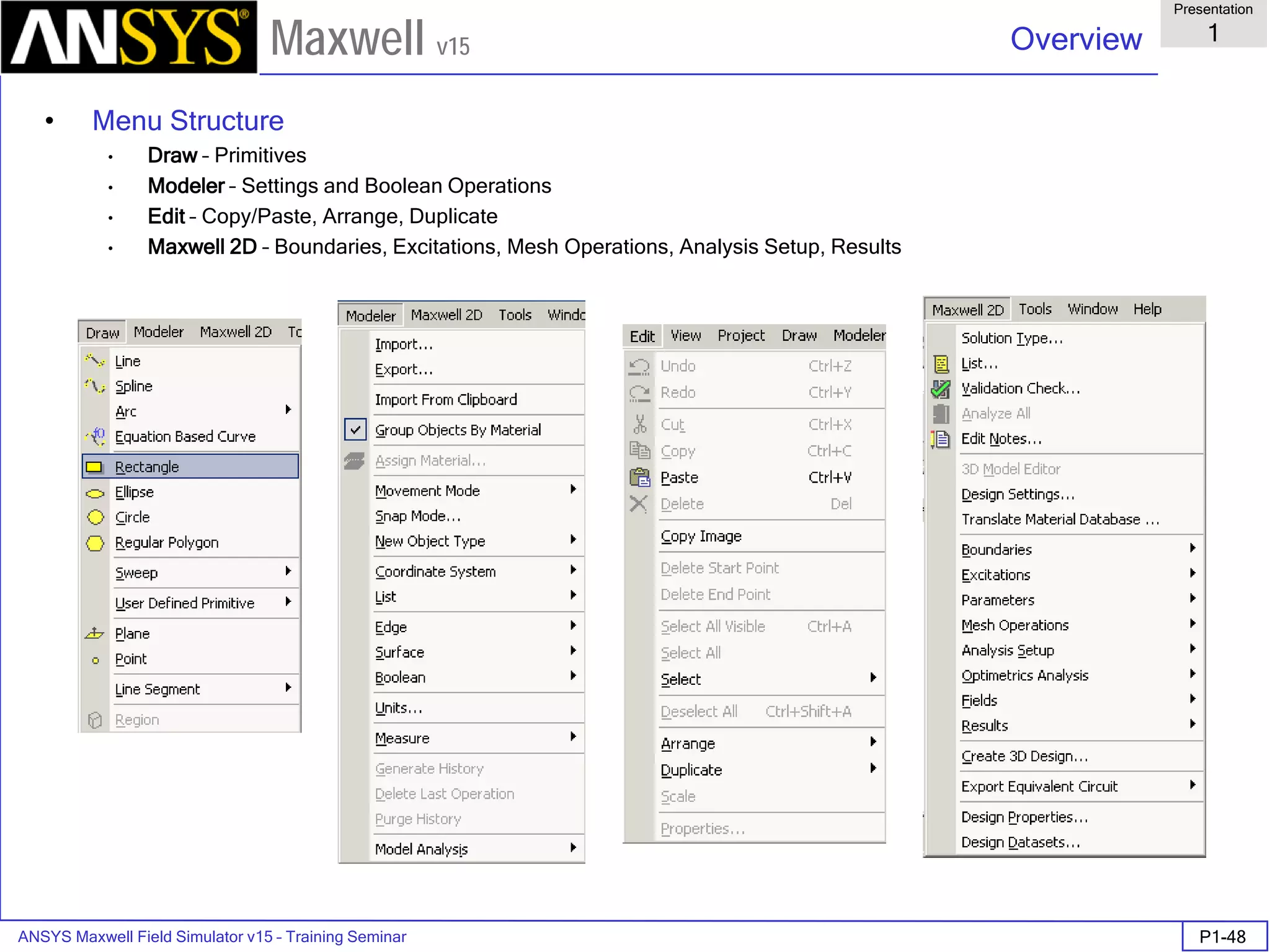
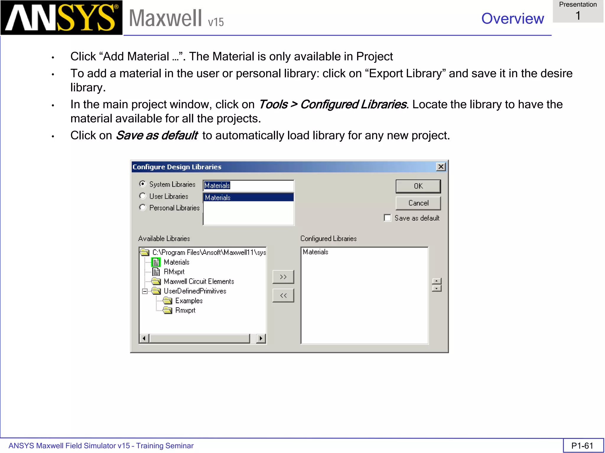
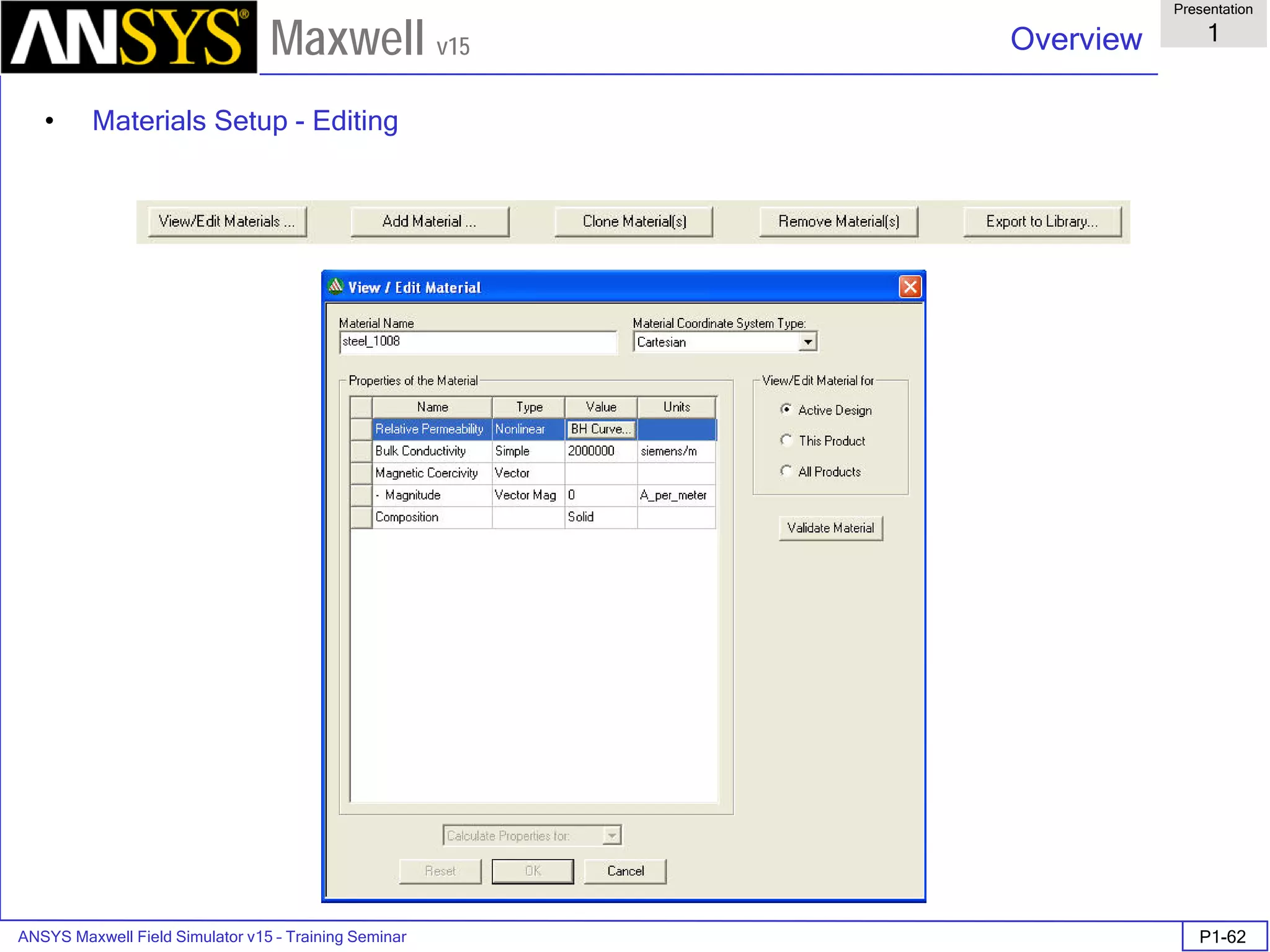
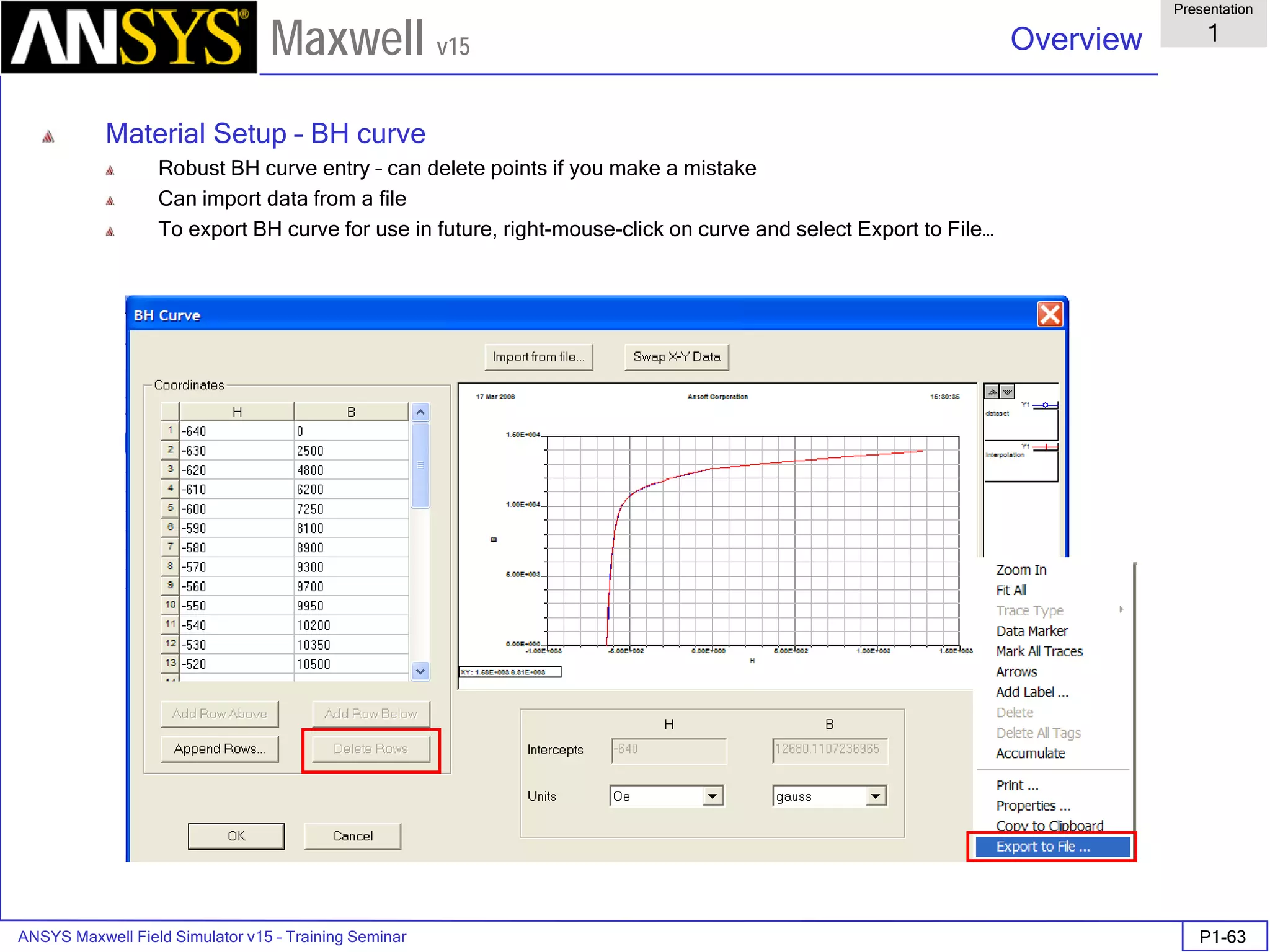
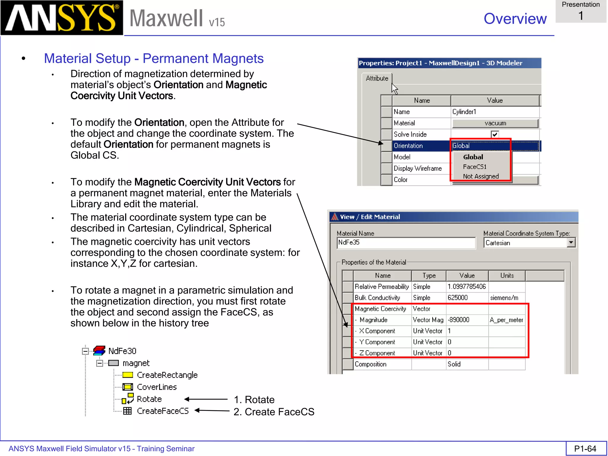
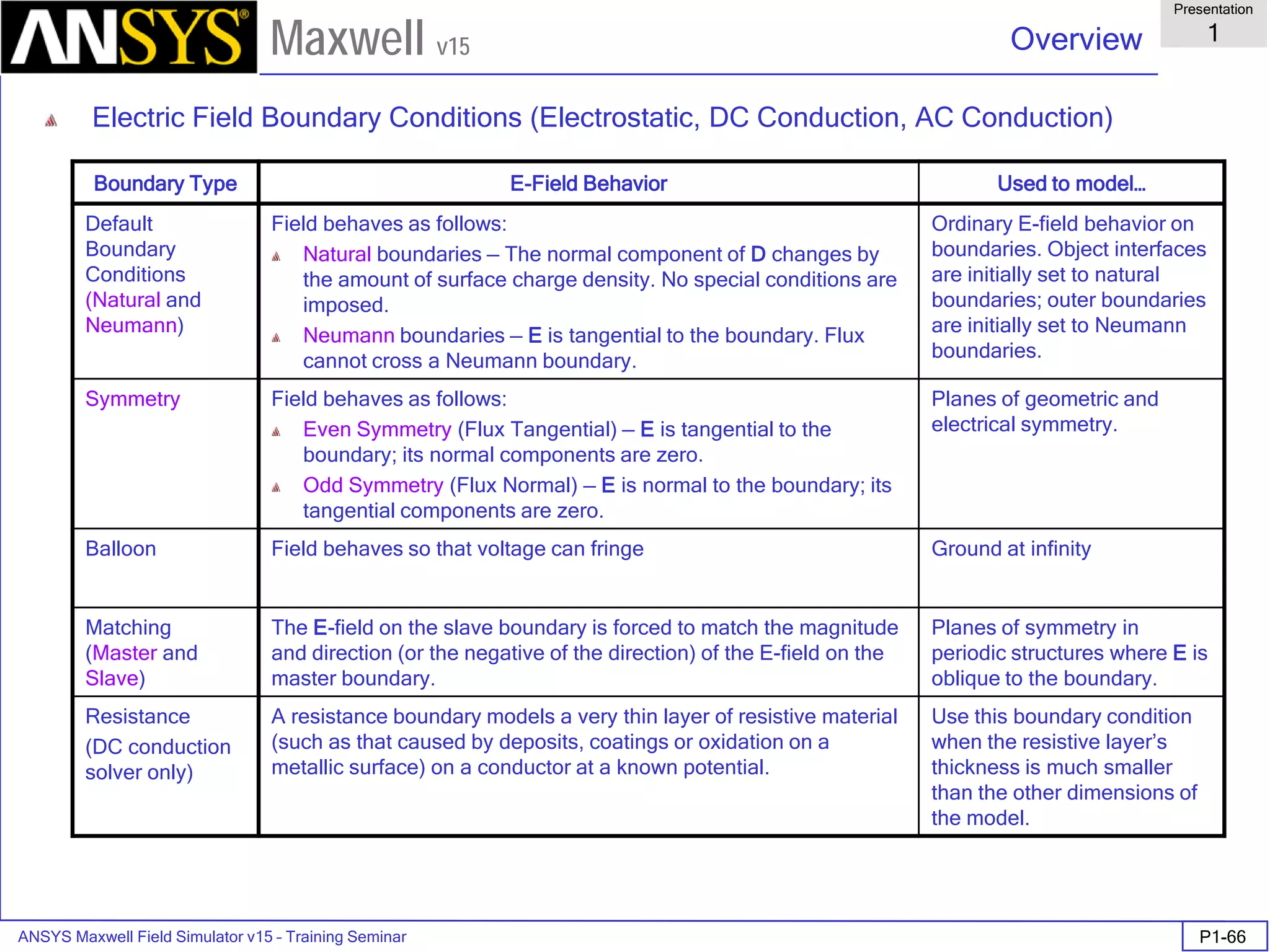
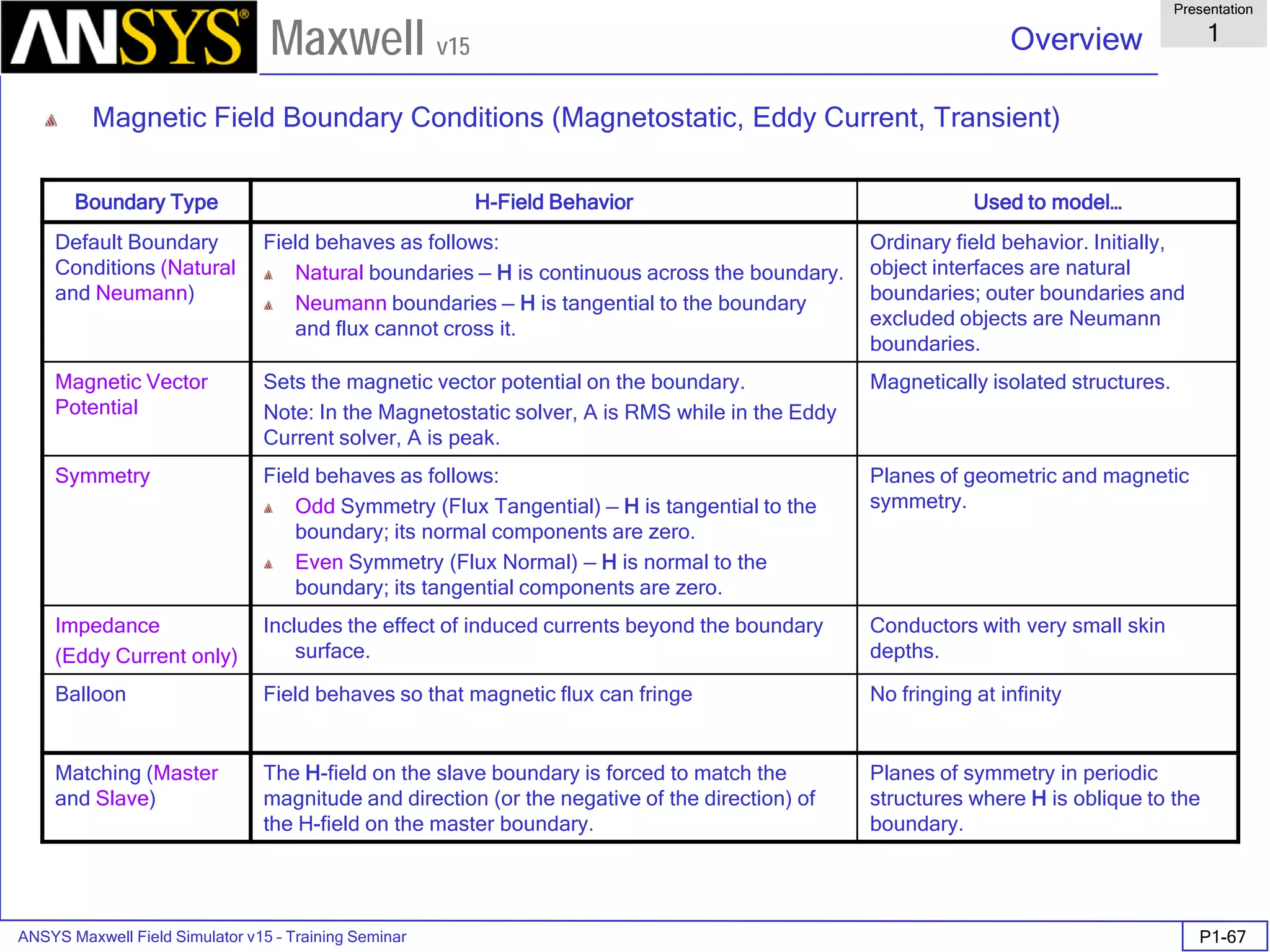
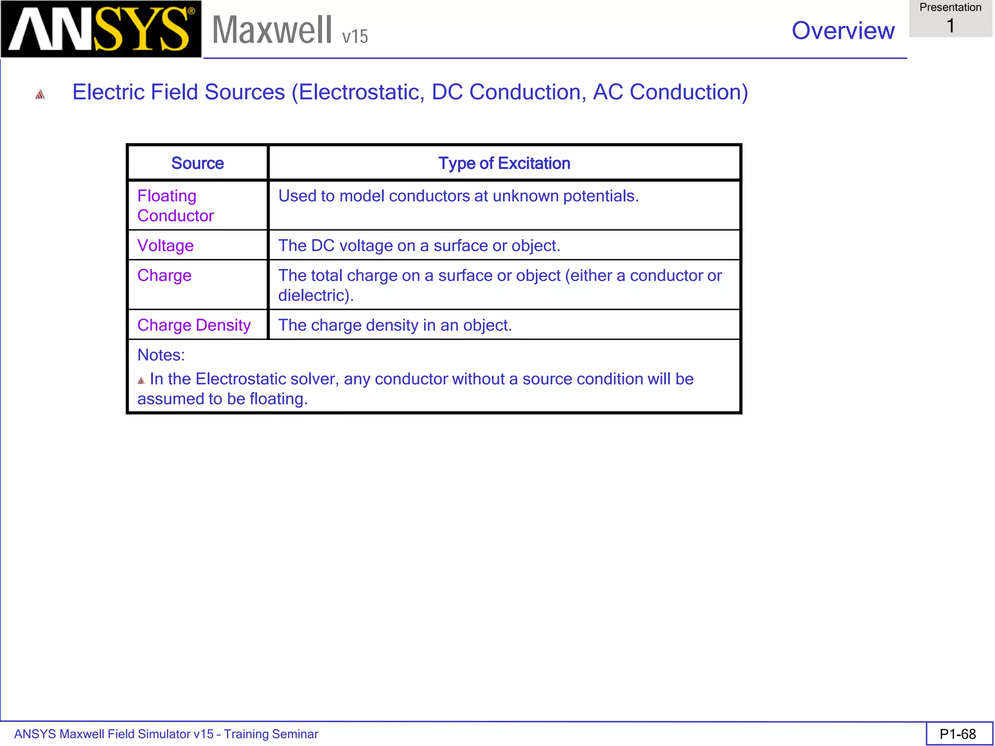
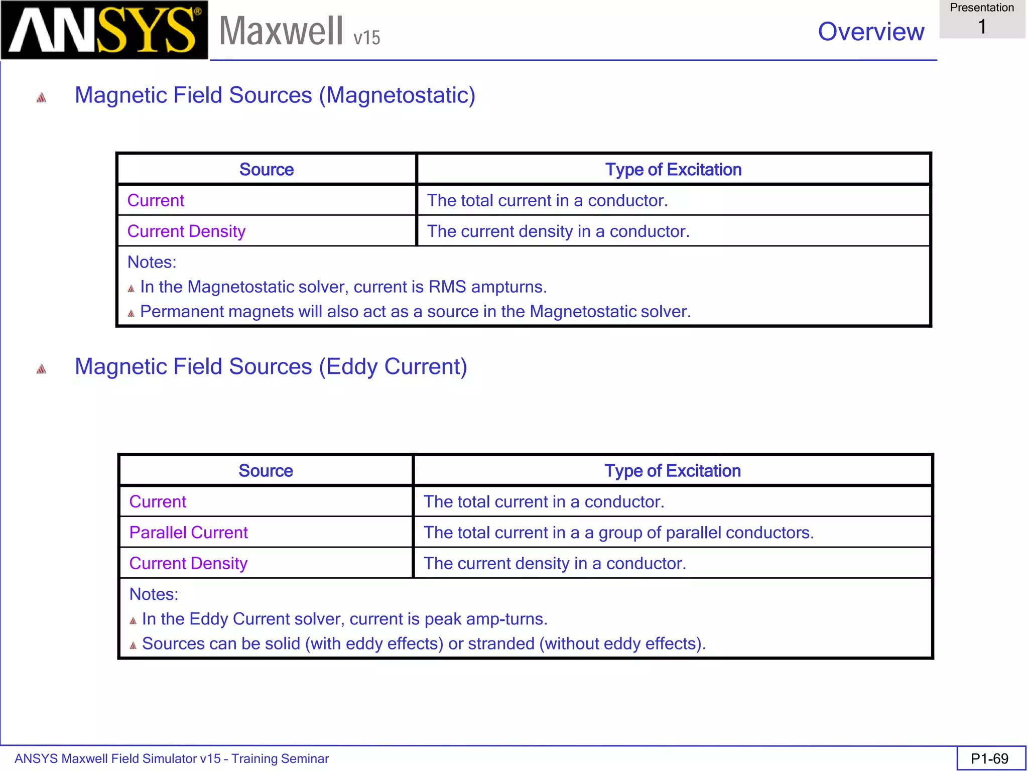
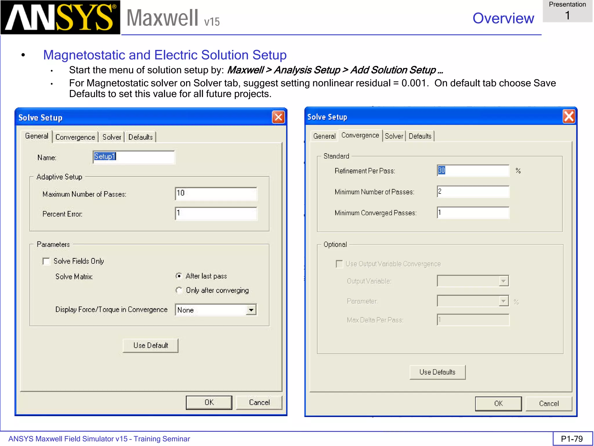
Overview
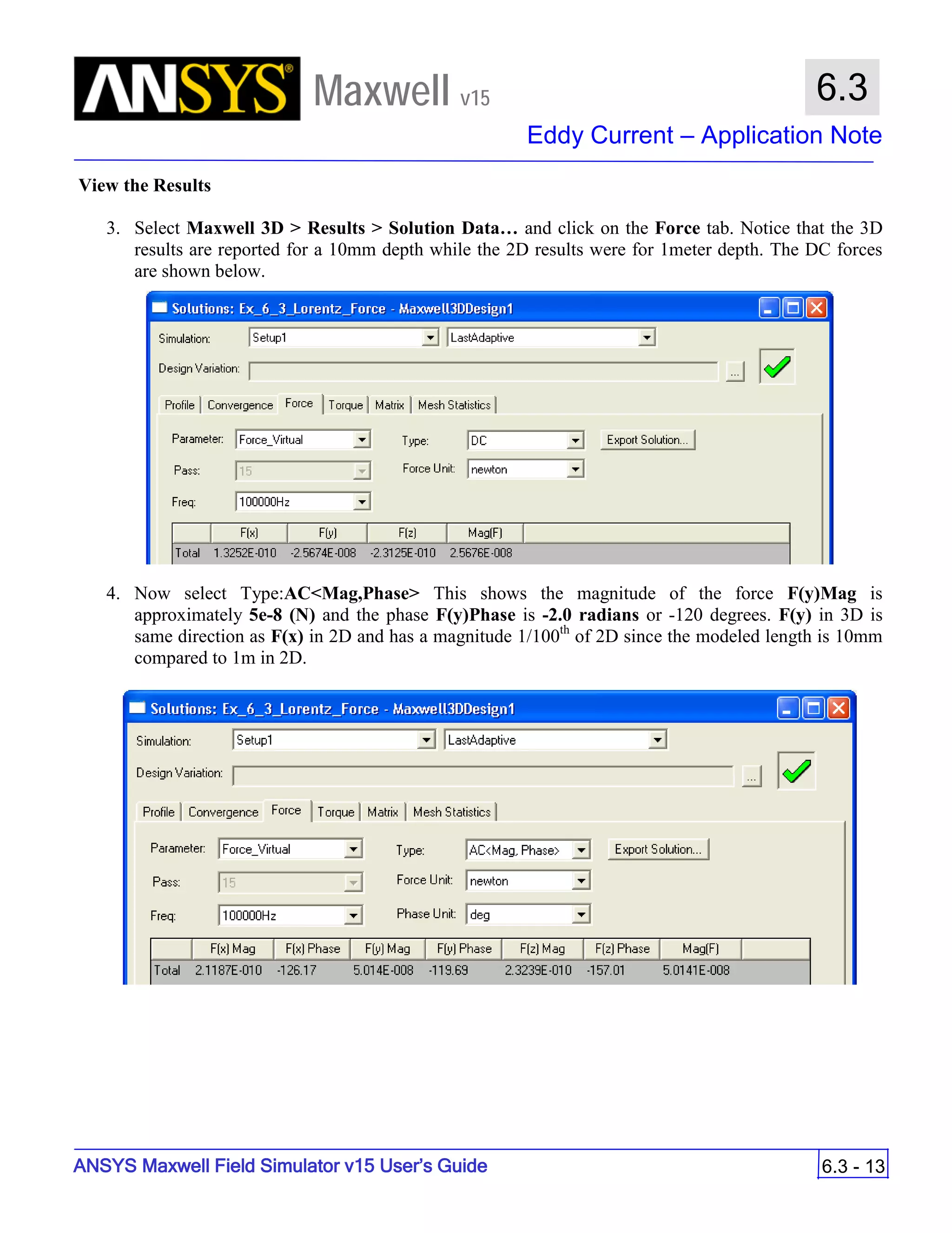
Presentation
1
Maxwell v15
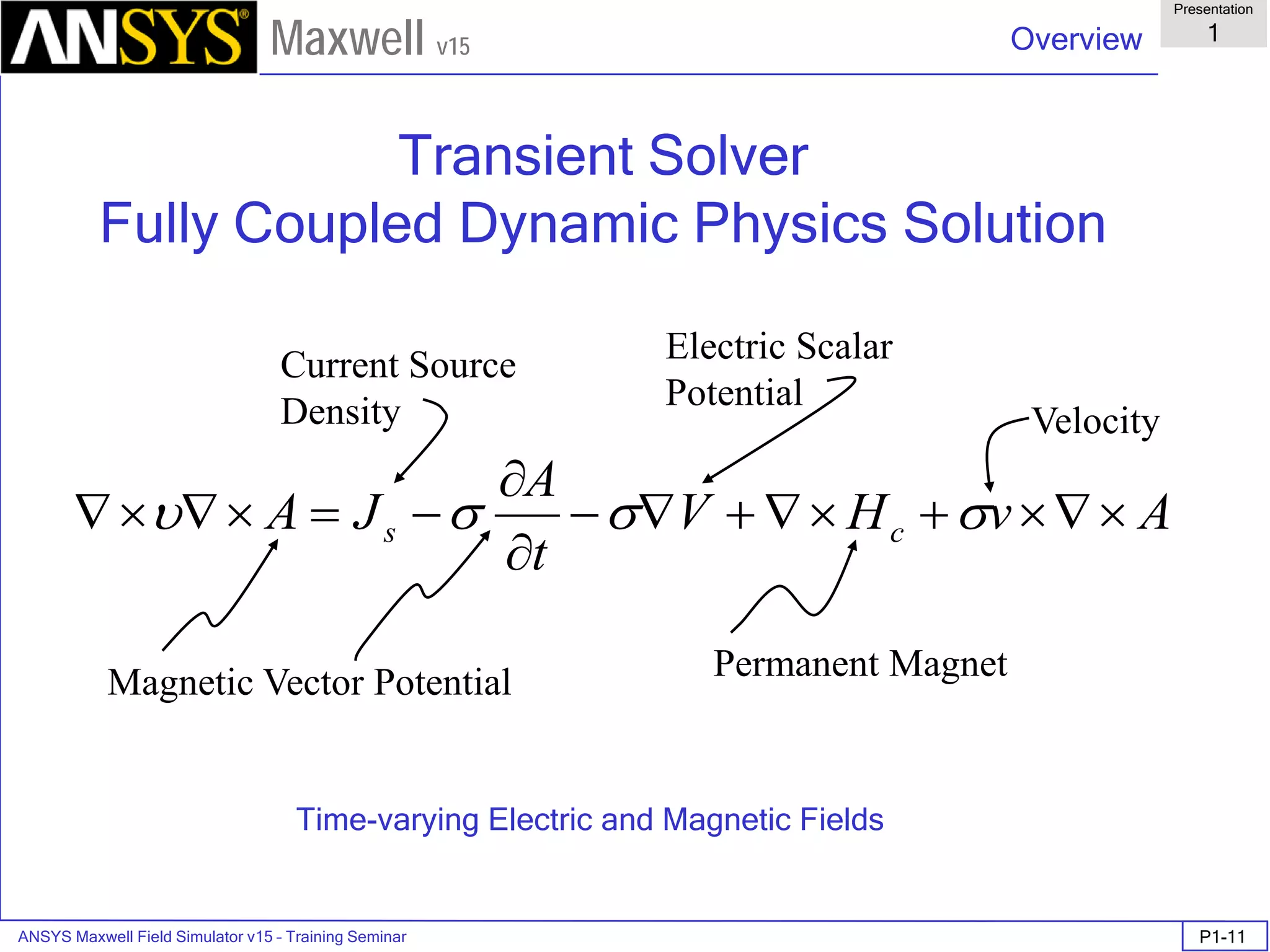
FEM Matrix Equation
• Now, over all the triangles, the result is a large, sparse matrix equation
• This can be solved using standard matrix solution techniques such as:
• Sparse Gaussian Elimination (direct solver)
• Incomplete Choleski Conjugate Gradient Method (ICCG iterative
solver)
[ ][ ] [ ]JAS =](https://image.slidesharecdn.com/completemaxwell2dv15-160410143735/75/Complete-maxwell-2d-v15-Latest-Version-11-2048.jpg)


![ANSYS Maxwell Field Simulator v15 – Training Seminar P1-65
Overview
Presentation
1
Maxwell v15
• Material Setup - Anisotropic Material Properties
• ε1, µ1, and σ1 are tensors in the X direction.
• ε2, µ2, and σ2 are tensors in the Y direction.
• ε3, µ3, and σ3 are tensors in the Z direction.
Note: Nonlinear anisotropic permeability not allowed in Maxwell 2D.
[ ] [ ] [ ]
=
=
=
3
2
1
3
2
1
3
2
1
00
00
00
,
00
00
00
,
00
00
00
σ
σ
σ
σ
µ
µ
µ
µ
ε
ε
ε
ε
Solver
Anisotropic
Permitivity
Anisotropic
Permeability
Anisotropic
Conductivity
Dielectric Loss
Tangent
Magnetic Loss
Tangent
Electrostatic yes no no no no
DC Conduction no no yes no no
AC Conduction yes no yes no no
Magnetostatic no yes no no no
Eddy Current no yes no no no
Transient no yes no no no](https://image.slidesharecdn.com/completemaxwell2dv15-160410143735/75/Complete-maxwell-2d-v15-Latest-Version-68-2048.jpg)


![ANSYS Maxwell Field Simulator v15 – Training Seminar P1-100
Overview
Presentation
1
Maxwell v15
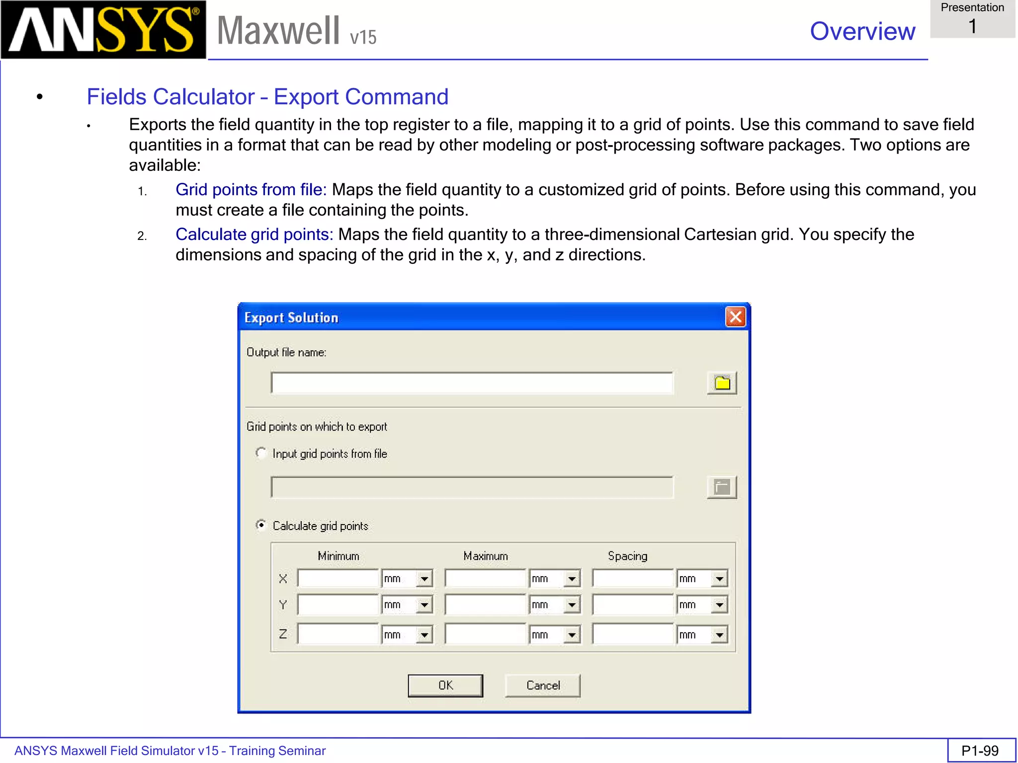
• Export to Grid
• Vector data <Ex,Ey,Ez>
• Min: [0 0 0]
• Max: [2 2 2]
• Spacing: [1 1 1]
• Space delimited ASCII file saved in
project subdirectory
Vector data "<Ex,Ey,Ez>"
Grid Output Min: [0 0 0] Max: [2 2 2] Grid Size: [1 1 1
0 0 0 -71.7231 -8.07776 128.093
0 0 1 -71.3982 -1.40917 102.578
0 0 2 -65.76 -0.0539669 77.9481
0 1 0 -259.719 27.5038 117.572
0 1 1 -248.088 16.9825 93.4889
0 1 2 -236.457 6.46131 69.4059
0 2 0 -447.716 159.007 -8.6193
0 2 1 -436.085 -262.567 82.9676
0 2 2 -424.454 -236.811 58.8847
1 0 0 -8.91719 -241.276 120.392
1 0 1 -8.08368 -234.063 94.9798
1 0 2 -7.25016 -226.85 69.5673
1 1 0 -271.099 -160.493 129.203
1 1 1 -235.472 -189.125 109.571
1 1 2 -229.834 -187.77 84.9415
1 2 0 -459.095 -8.55376 2.12527
1 2 1 -447.464 -433.556 94.5987
1 2 2 -435.833 -407.8 70.5158
2 0 0 101.079 -433.897 -18.5698
2 0 1 -327.865 -426.684 95.8133
2 0 2 -290.824 -419.471 70.4008
2 1 0 -72.2234 -422.674 -9.77604
2 1 1 -495.898 -415.461 103.026
2 1 2 -458.857 -408.248 77.6138
2 2 0 -470.474 -176.115 12.8698
2 2 1 -613.582 -347.994 83.2228
2 2 2 -590.326 -339.279 63.86](https://image.slidesharecdn.com/completemaxwell2dv15-160410143735/75/Complete-maxwell-2d-v15-Latest-Version-103-2048.jpg)


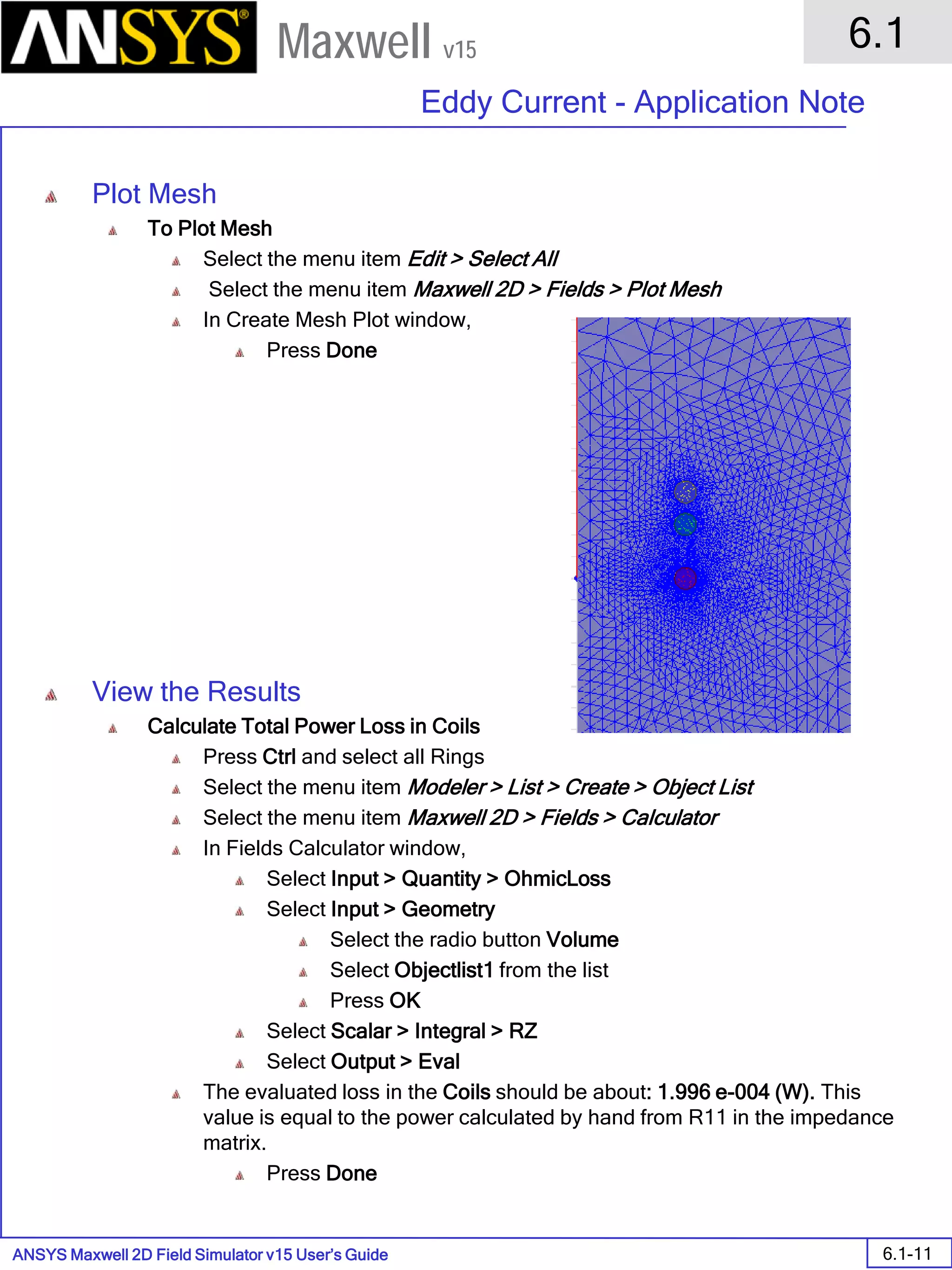
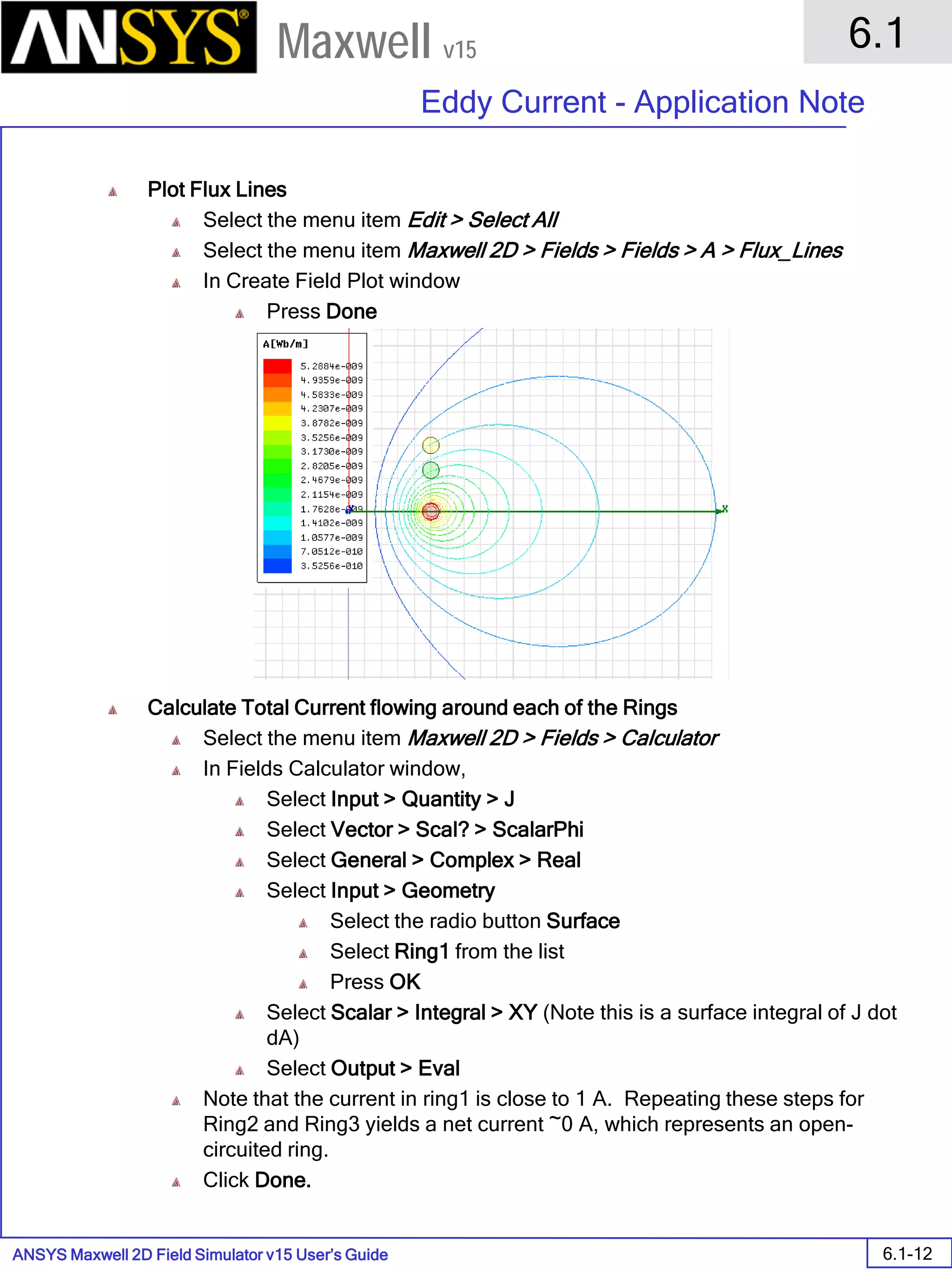
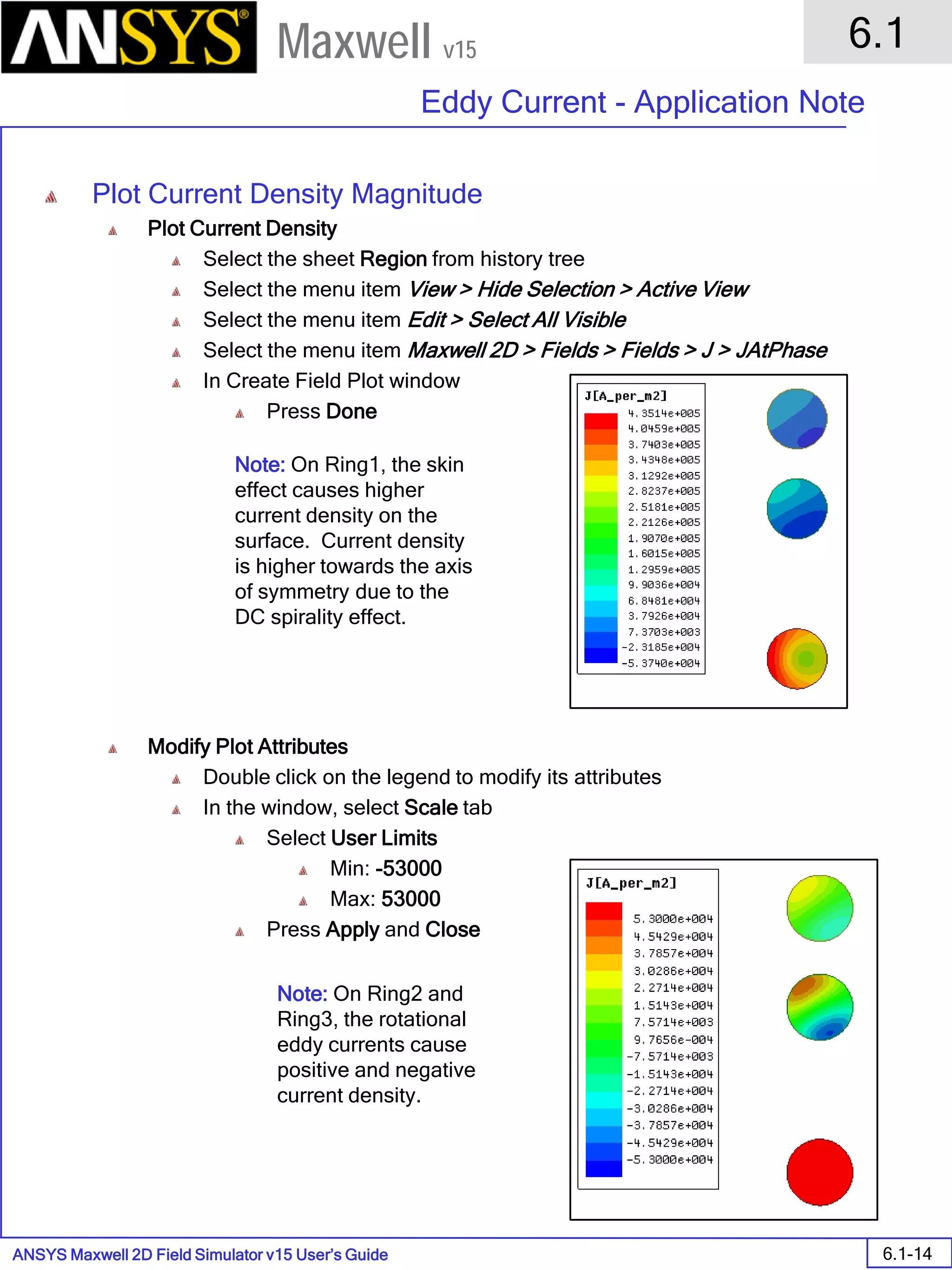
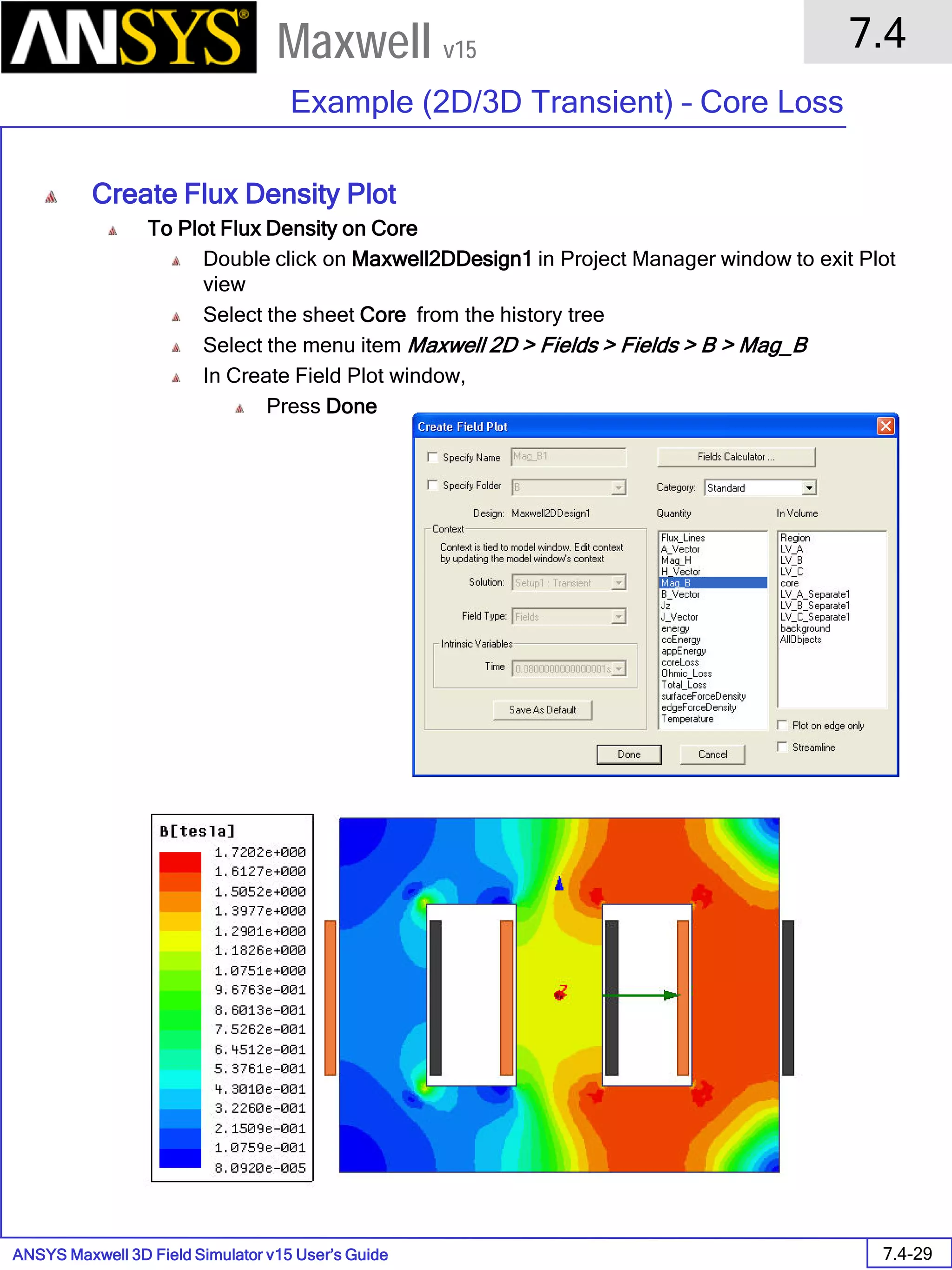
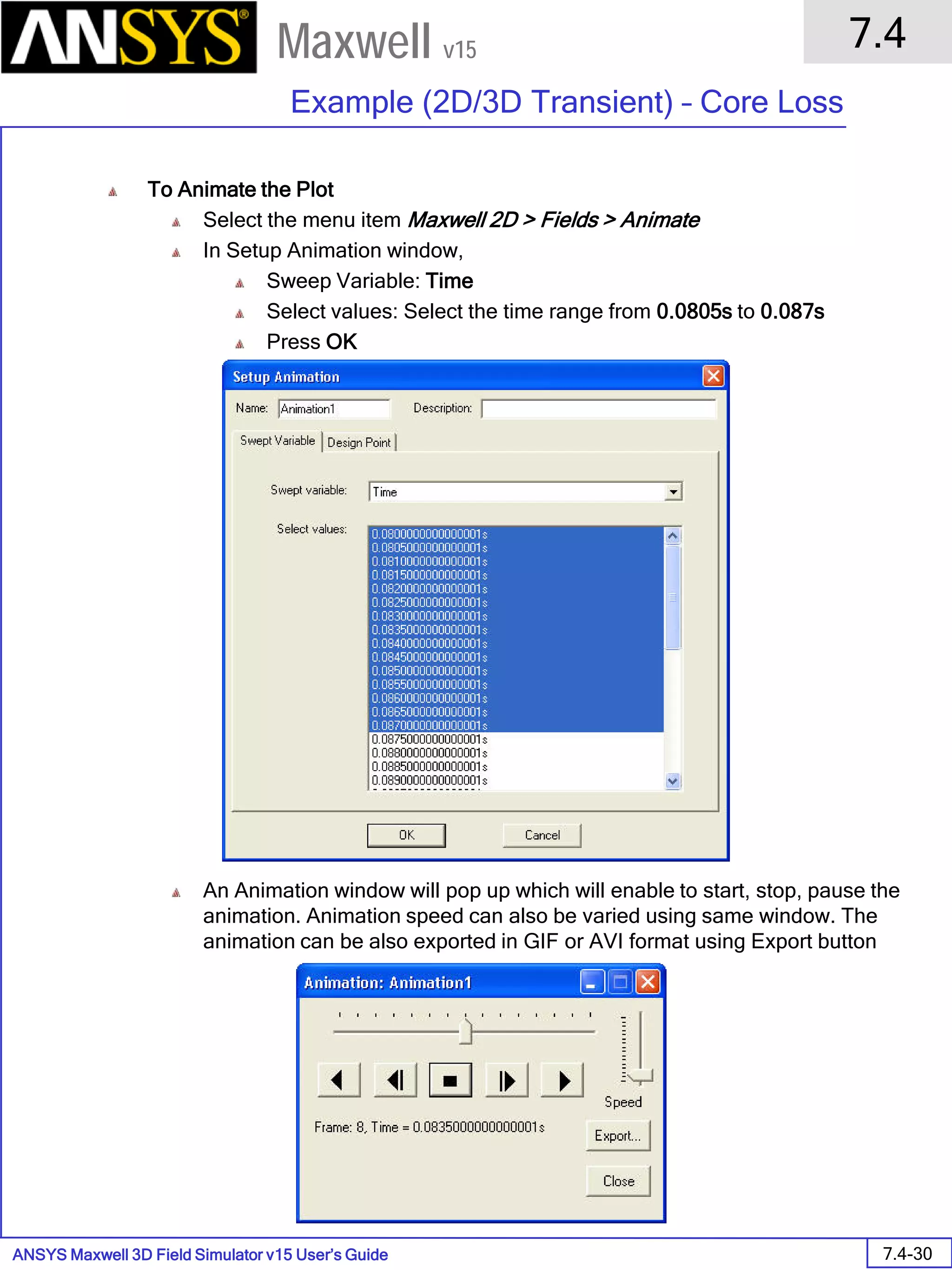
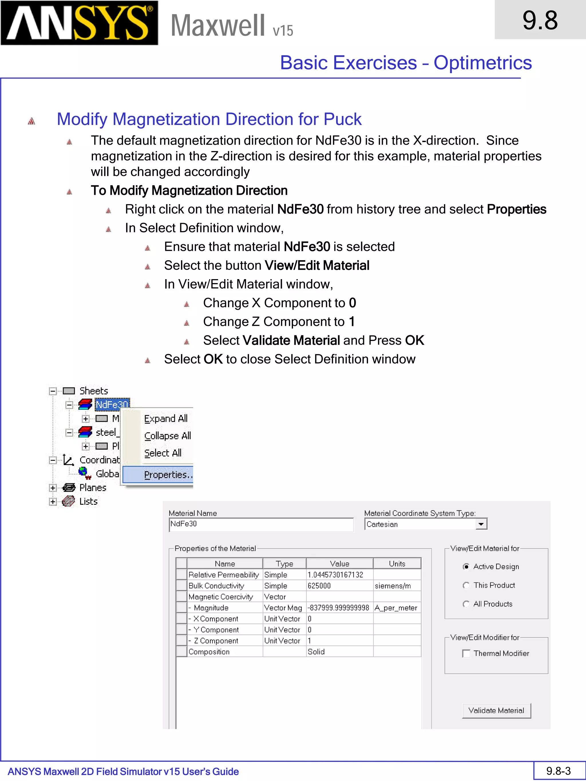
![ANSYS Maxwell 2D Field Simulator v15 User’s Guide
6.1
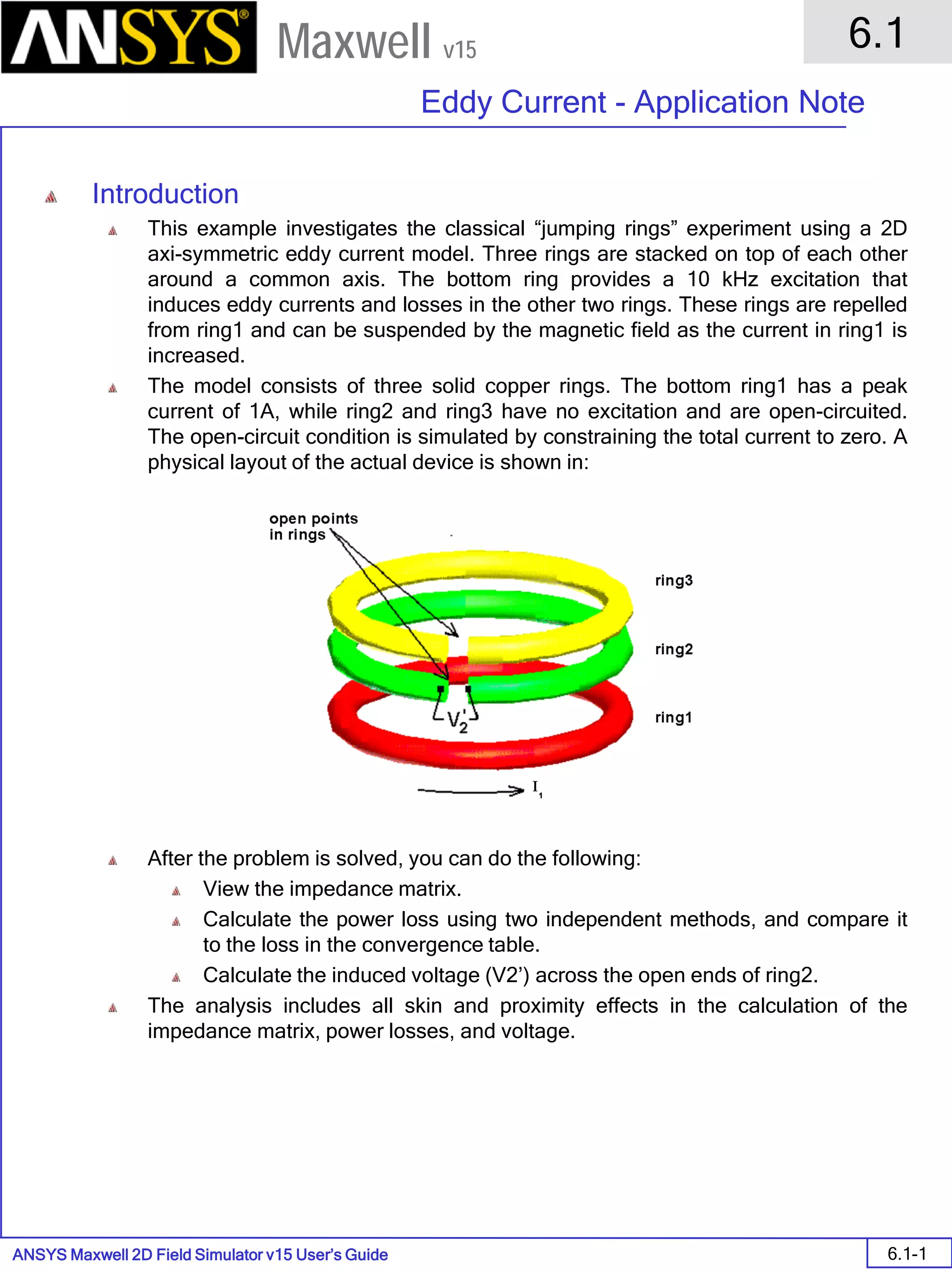
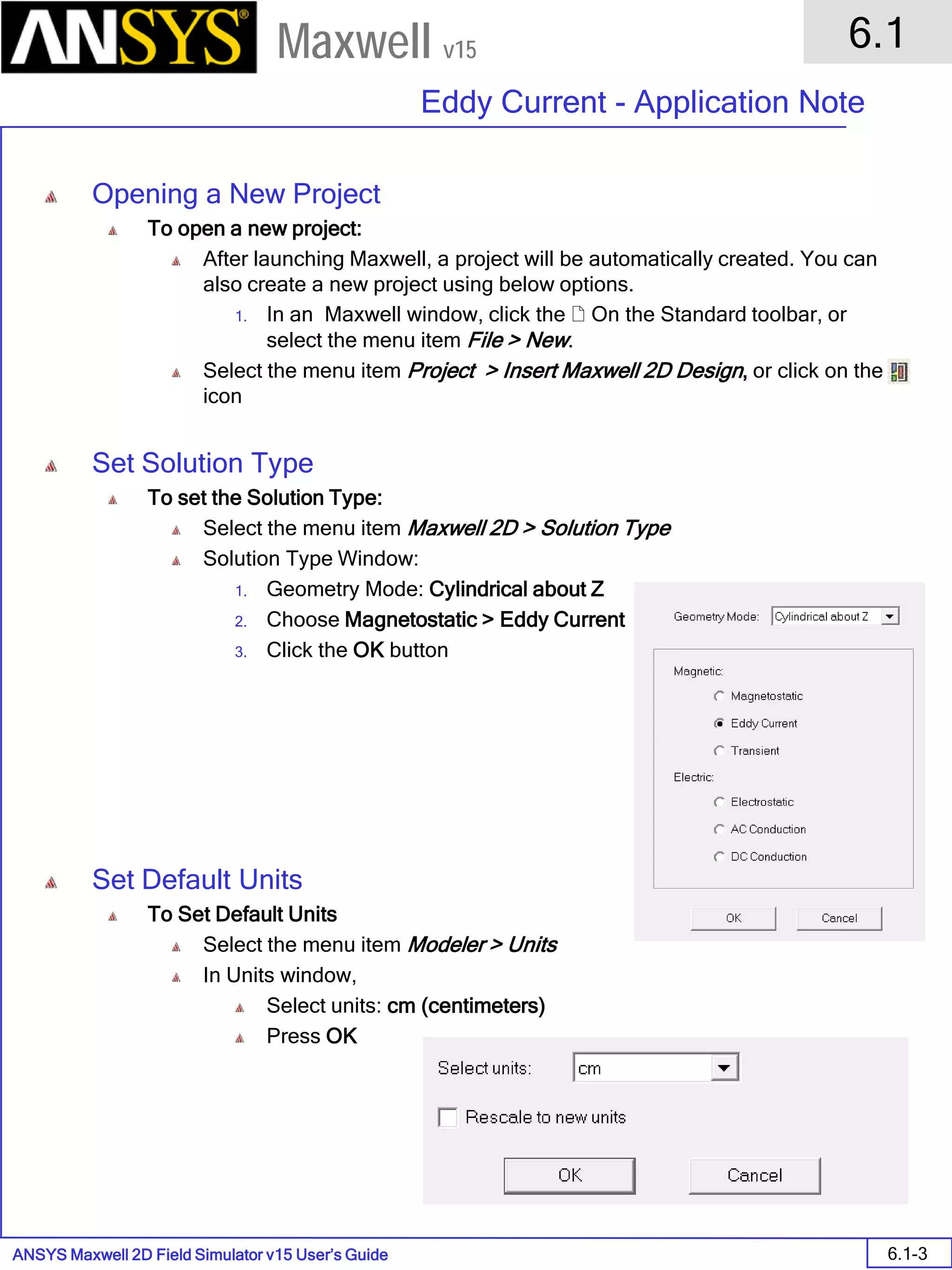
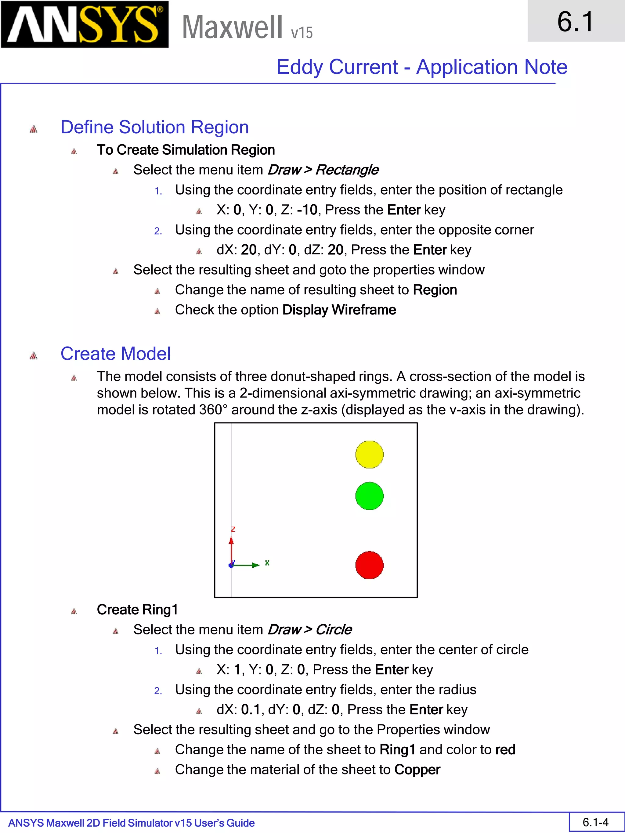
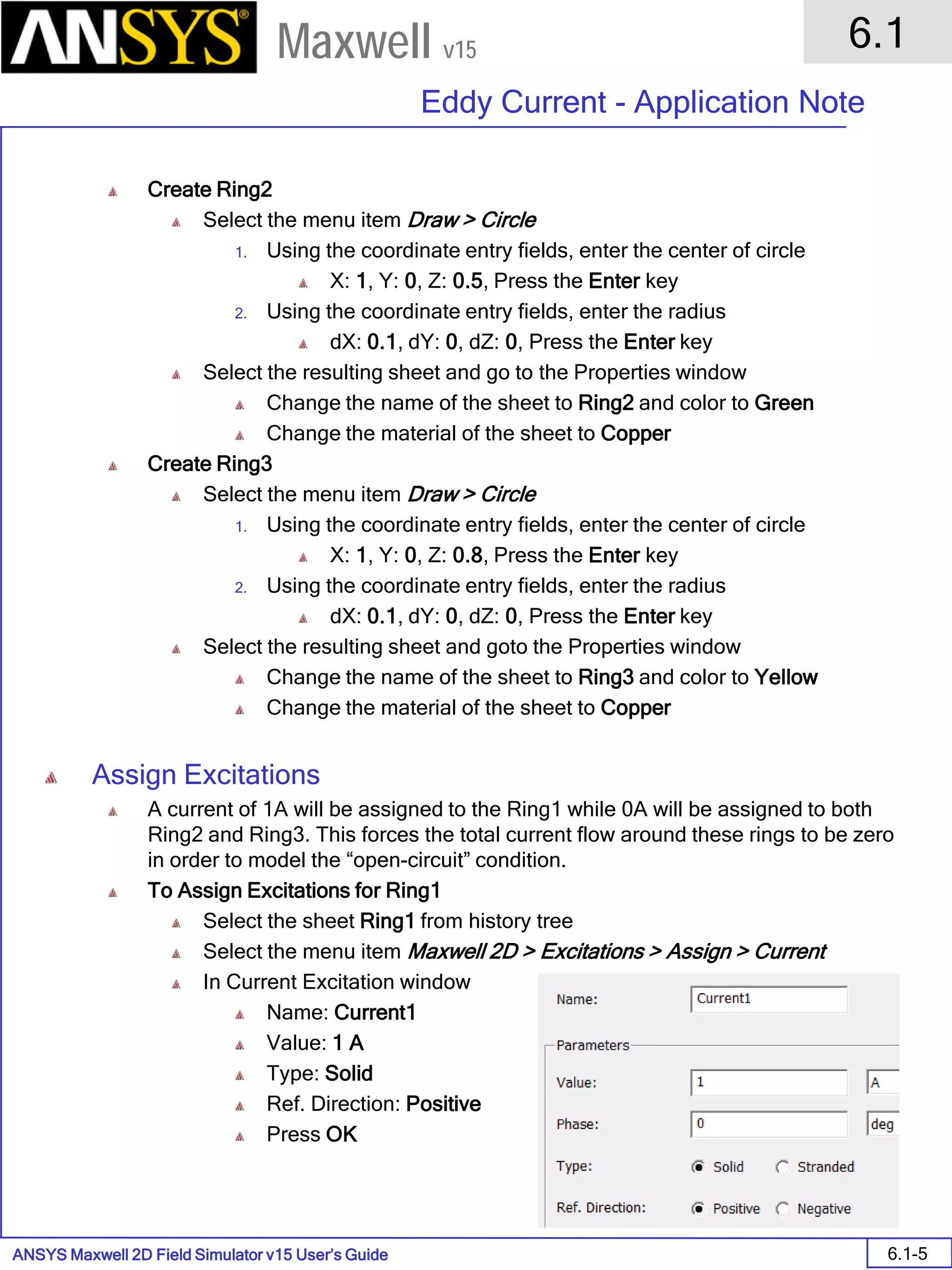
Eddy Current - Application Note
6.1-7
Maxwell v15
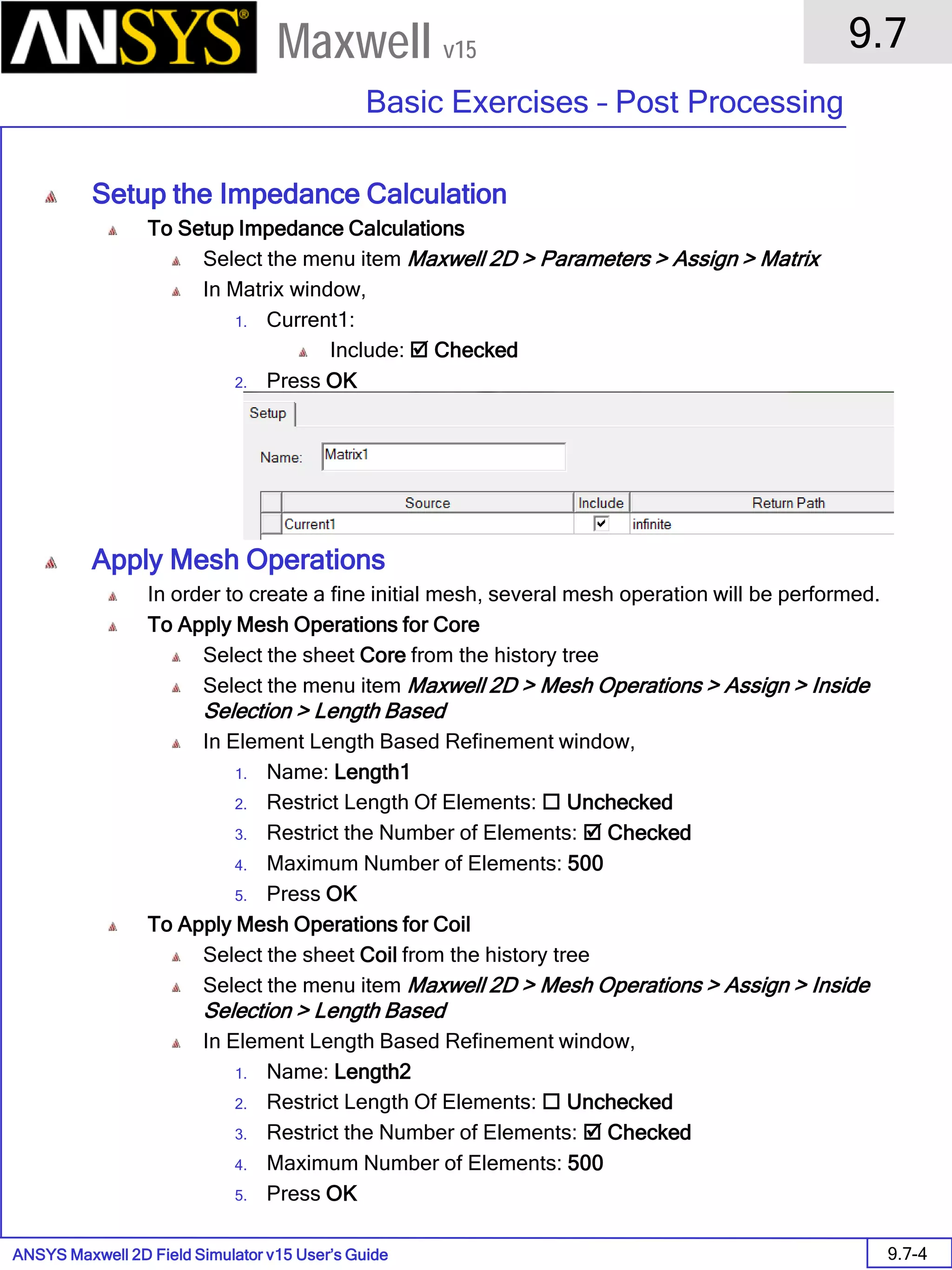
Assign Matrix Parameters
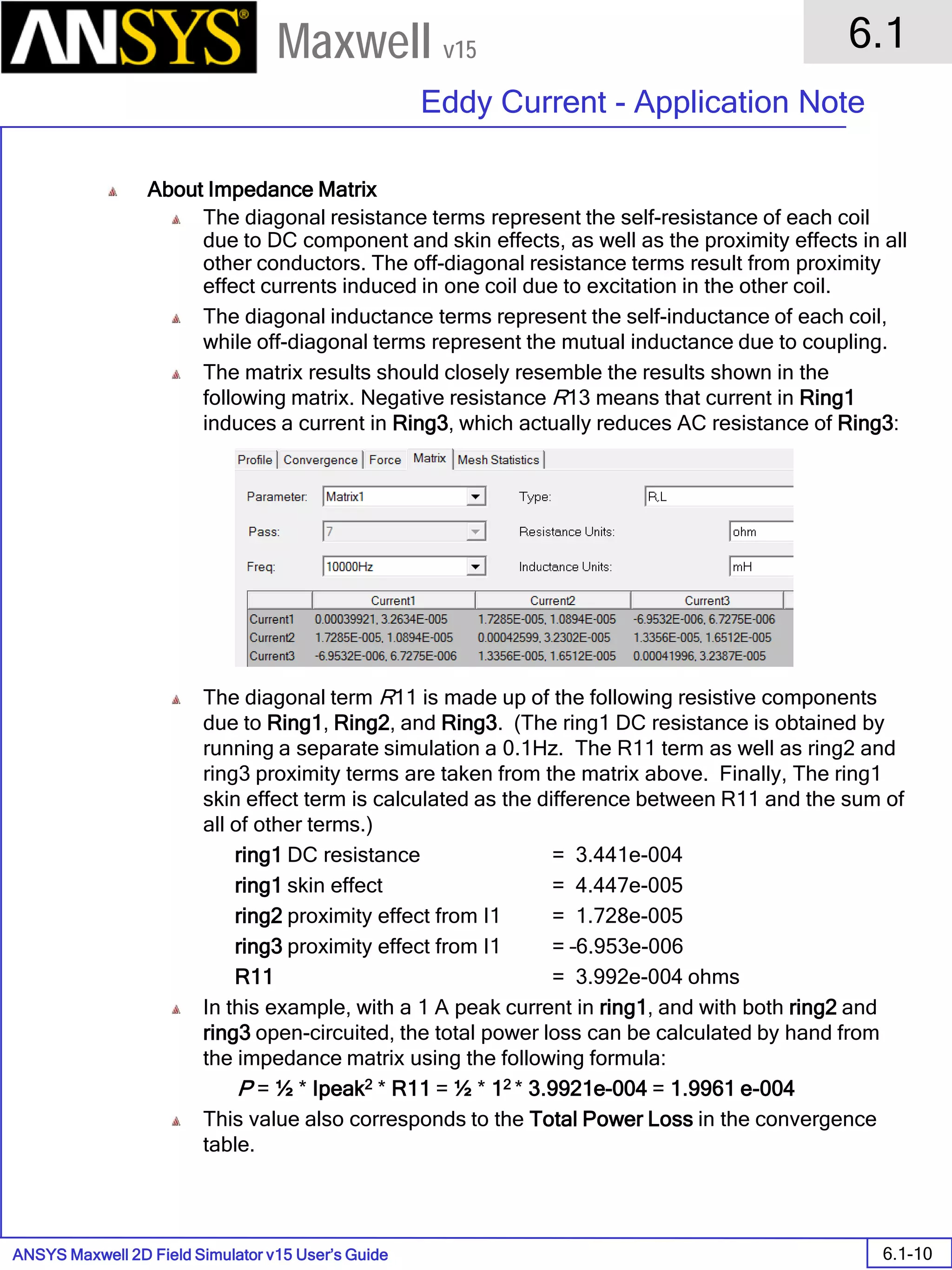
In this example, the compete [3x3] impedance matrix will be calculated. This is
done by setting a parameter.
To Calculate Impedance Matrix
Select the menu item Maxwell 2D > Parameters > Assign > Matrix
In Matrix window,
For all current Sources
Include: Checked
Press OK
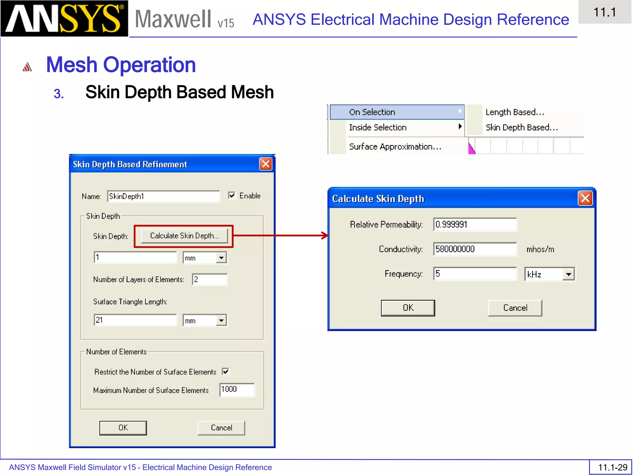
Compute the Skin Depth
Skin depth is a measure of how current density concentrates at the surface of a
conductor carrying an alternating current. It is a function of the permeability,
conductivity and frequency
Skin depth in meters is defined as follows:
where:
ω is the angular frequency, which is equal to 2πf. (f is the source frequency
which in this case is 10000Hz).
σ is the conductor’s conductivity; for copper its 5.8e7 S/m
µr is the conductor’s relative permeability; for copper its 1
µο is the permeability of free space, which is equal to 4π×10-7 A/m.
For the copper coils, the skin depth is approximately 0.066 cm which less than
the diameter of 0.200cm for the conductors.
σµωµ
δ
ro
2
=](https://image.slidesharecdn.com/completemaxwell2dv15-160410143735/75/Complete-maxwell-2d-v15-Latest-Version-114-2048.jpg)
![ANSYS Maxwell 2D Field Simulator v15 User’s Guide
6.1
Eddy Current - Application Note
6.1-9
Maxwell v15
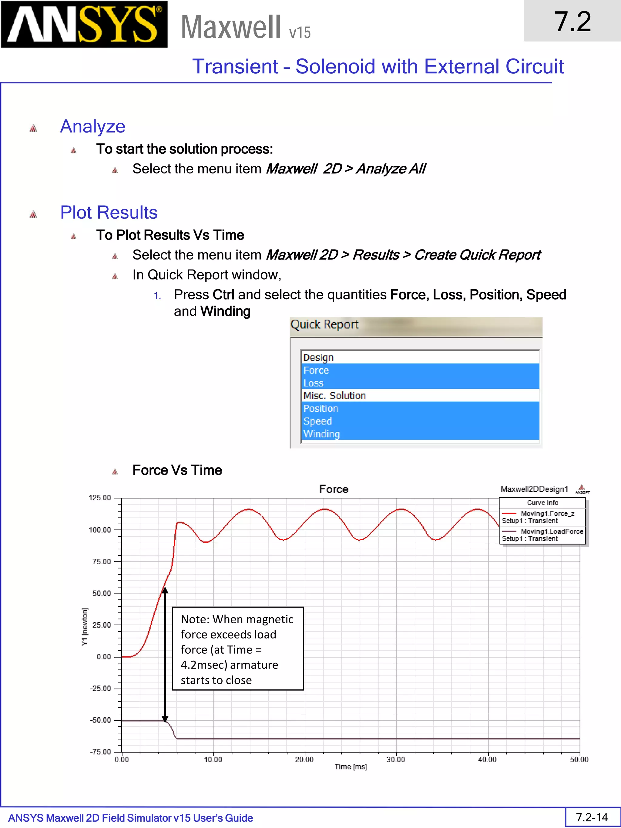
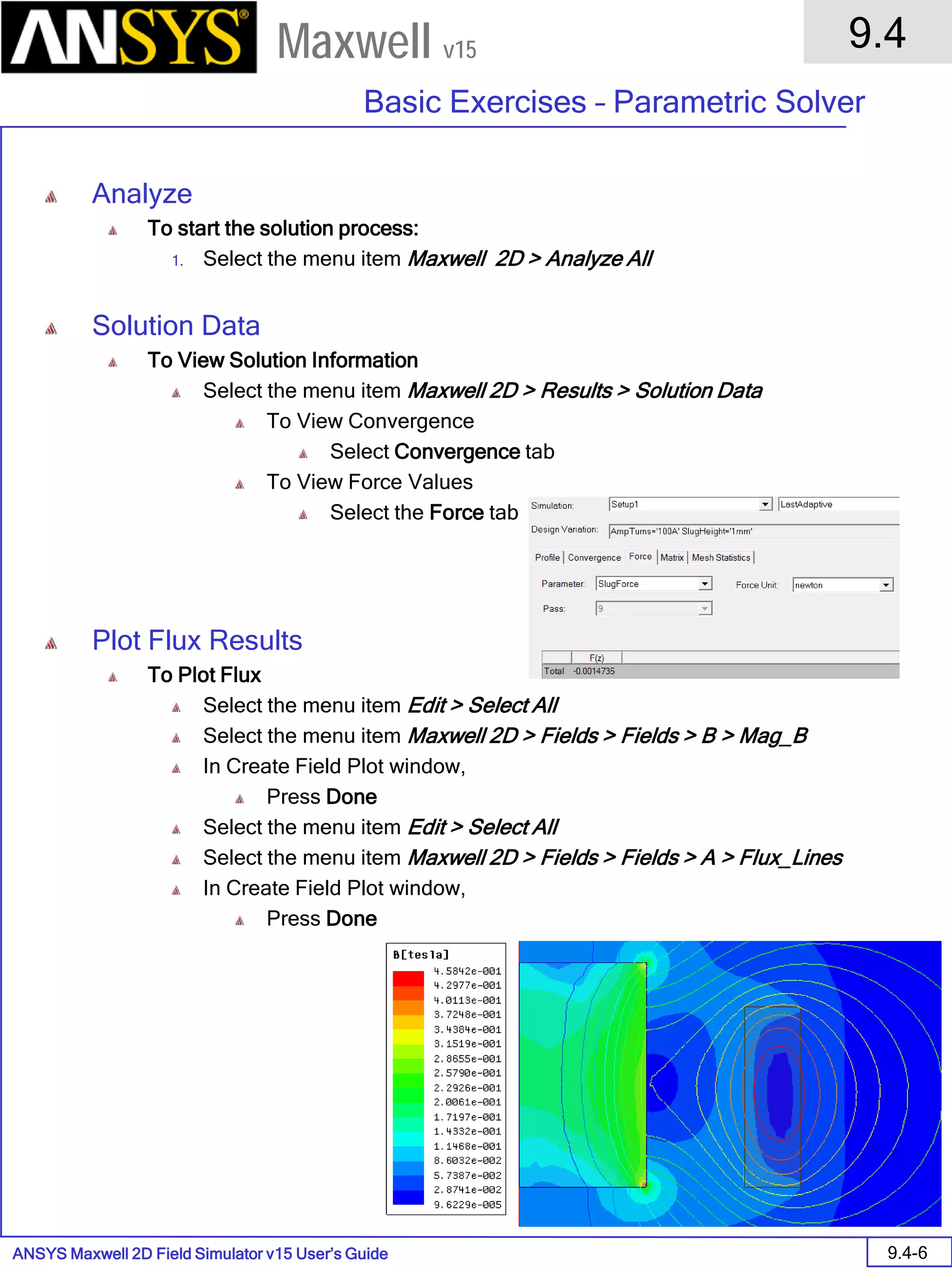
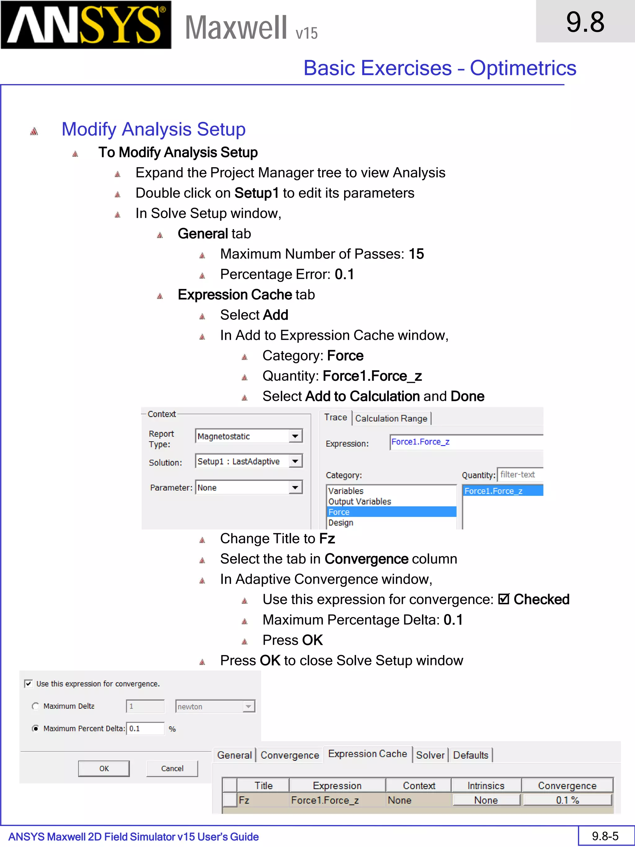
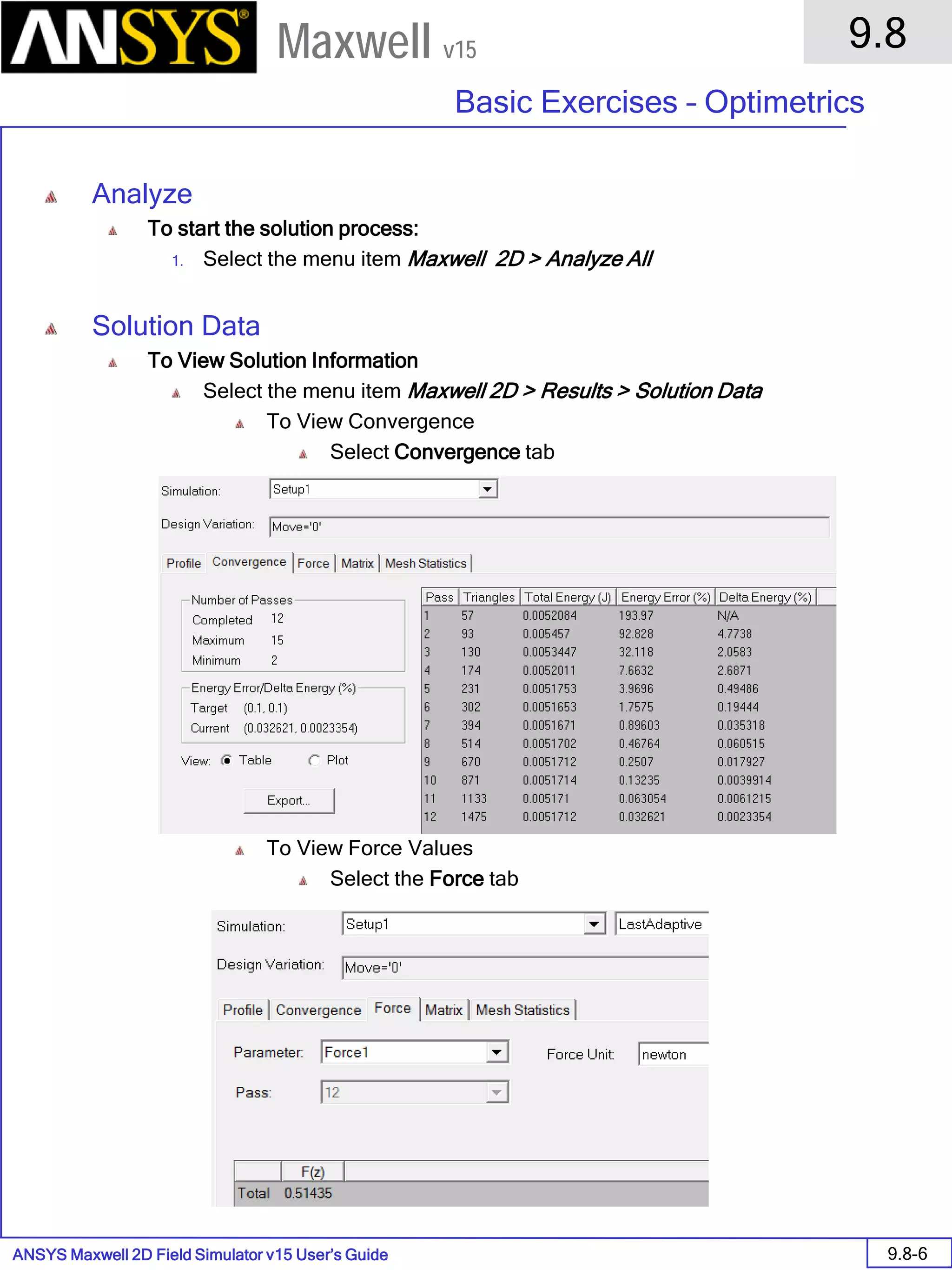
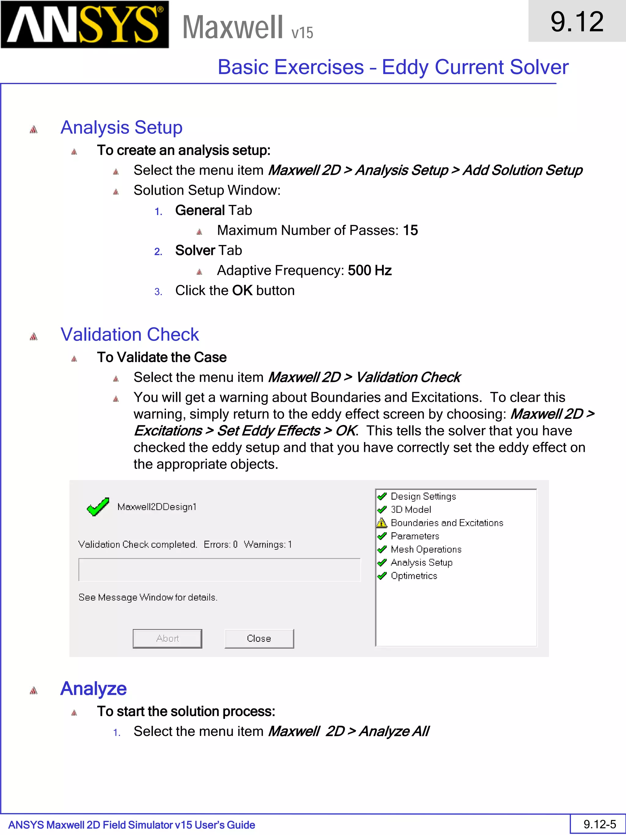
Analyze
To start the solution process:
1. Select the menu item Maxwell 2D > Analyze All
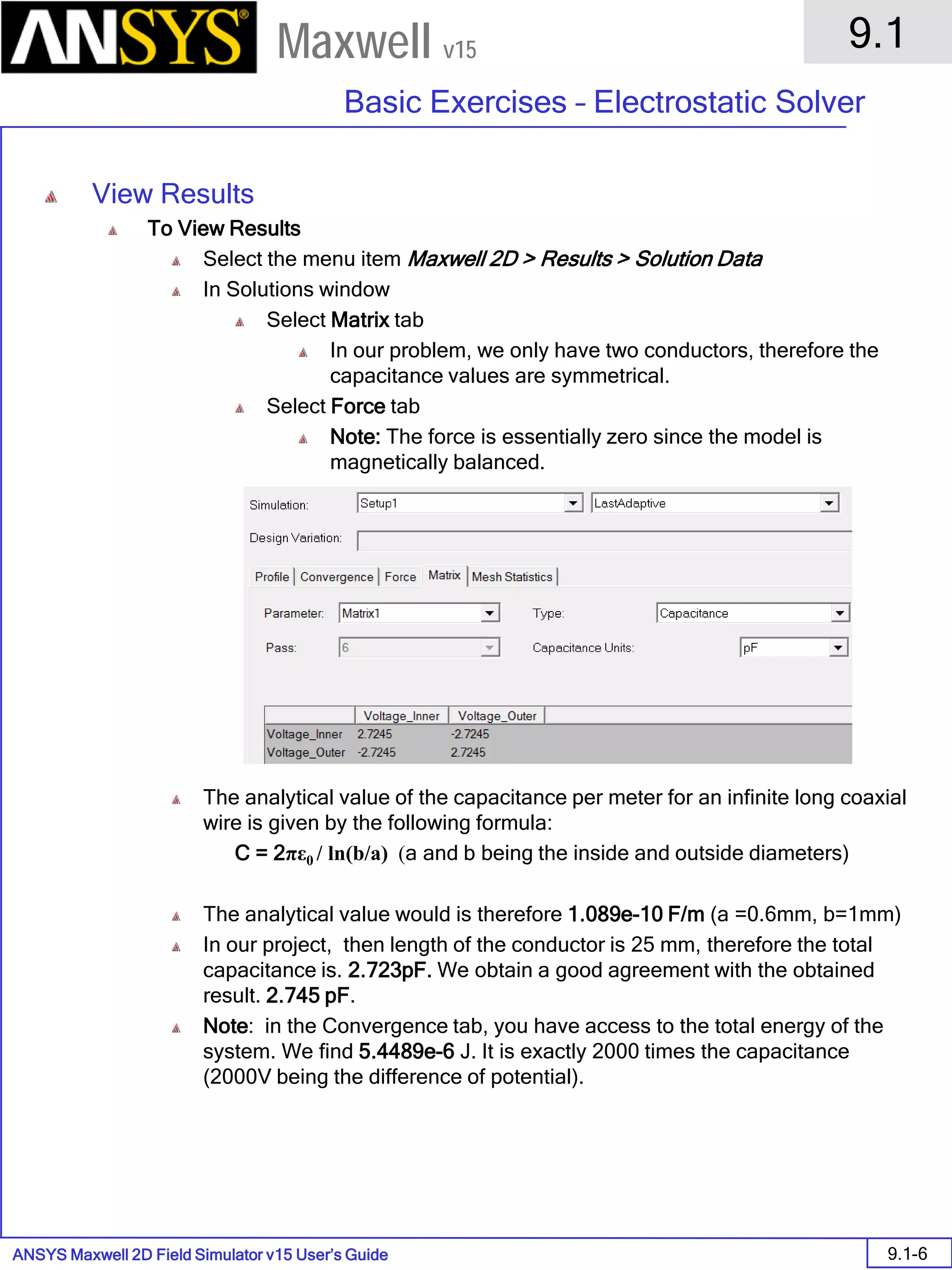
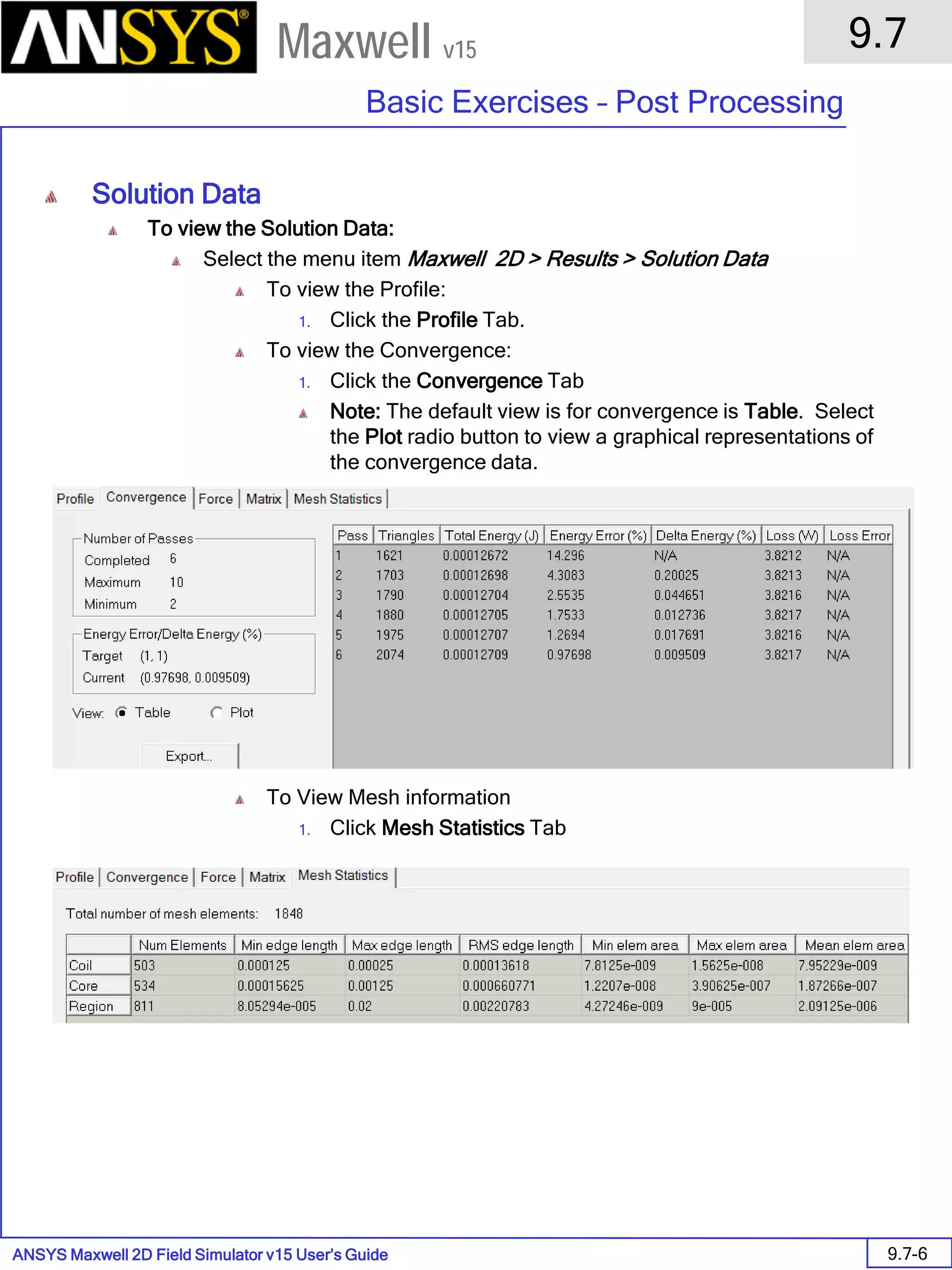
Solution Data
To View Solution Information
Select the menu item Maxwell 2D > Results > Solution Data
To View Convergence
Select the Convergence tab
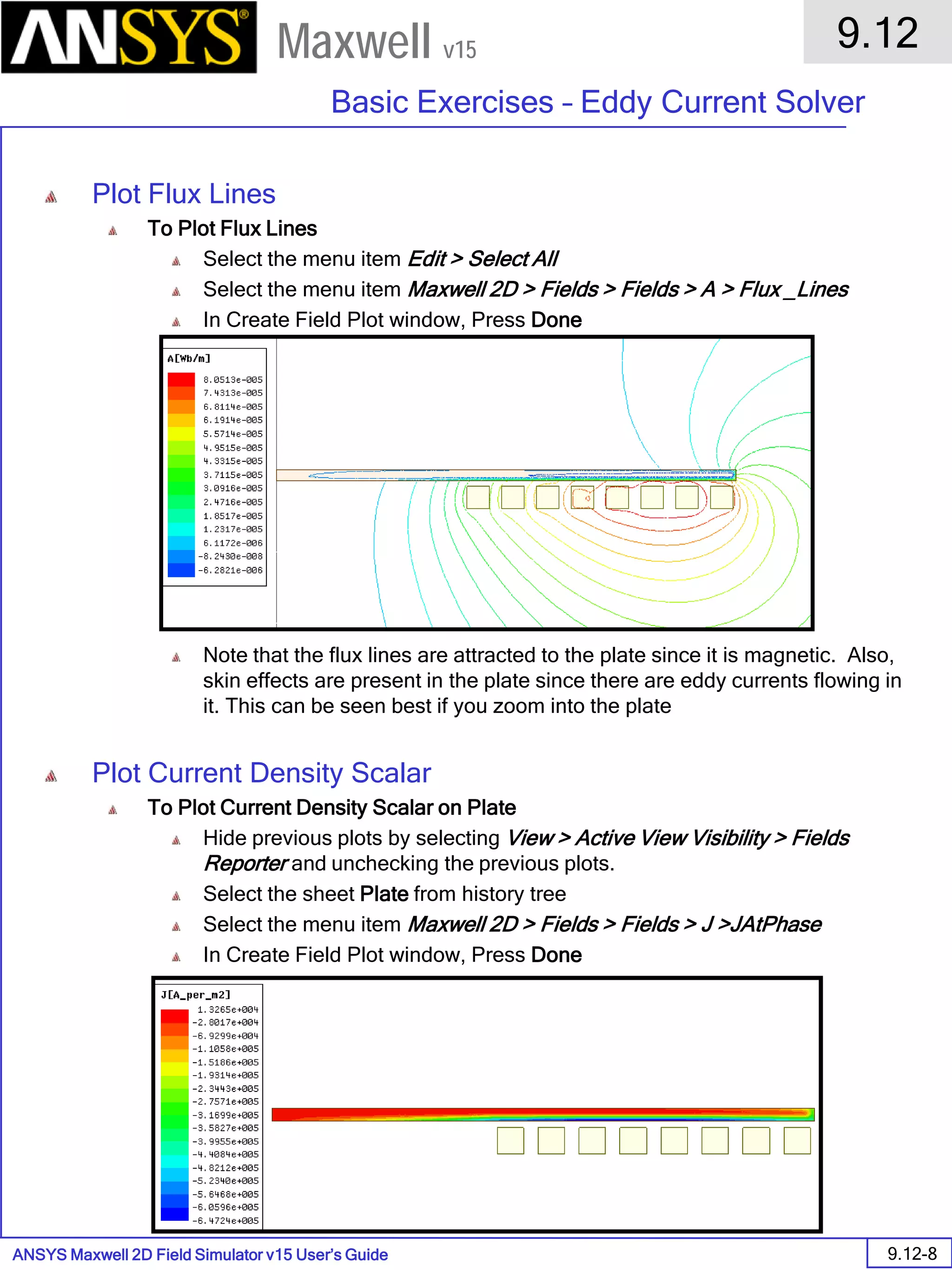
Note that the total loss is around 1.99e-004 Watts
To View Mesh information
Select the Mesh Statistics tab
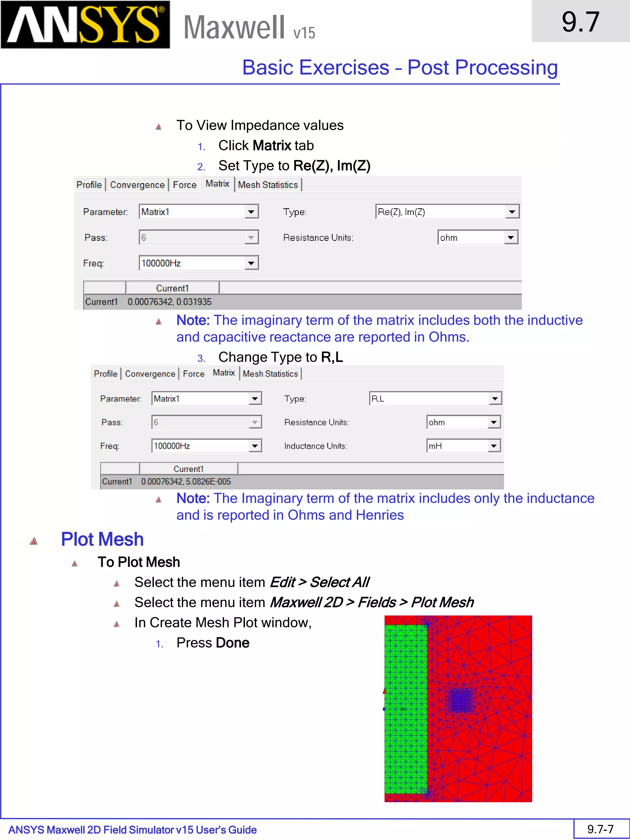
To View Impedance matrix
Select Matrix tab
By default, the results are displayed as [R, Z] but can be also
shown as [R, L] or as coupling coefficients.
333332323131
232322222121
131312121111
,,,
,,,
,,,
LRLRLR
LRLRLR
LRLRLR](https://image.slidesharecdn.com/completemaxwell2dv15-160410143735/75/Complete-maxwell-2d-v15-Latest-Version-116-2048.jpg)


![ANSYS Maxwell 2D Field Simulator v15 User’s Guide
9.12
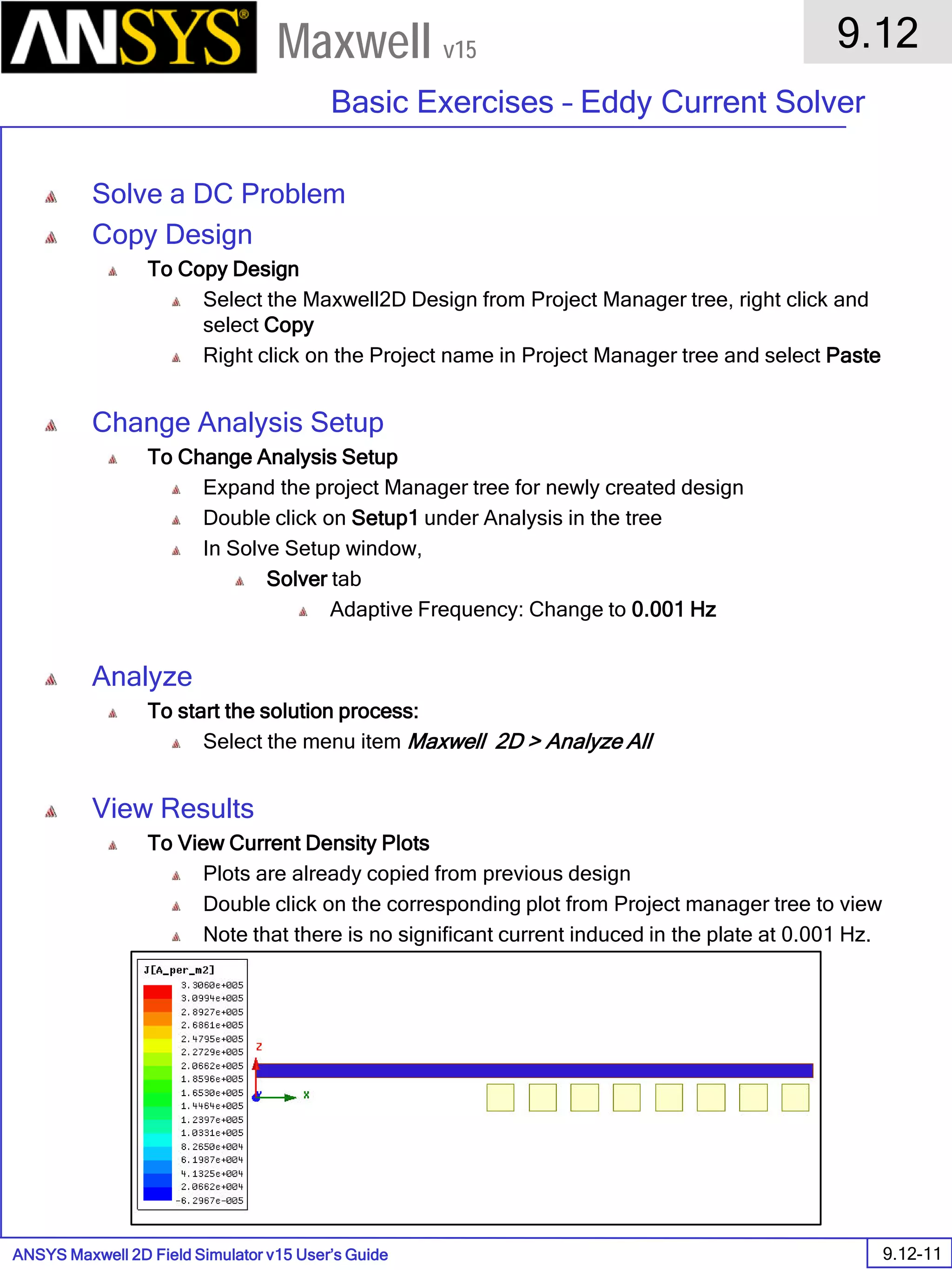
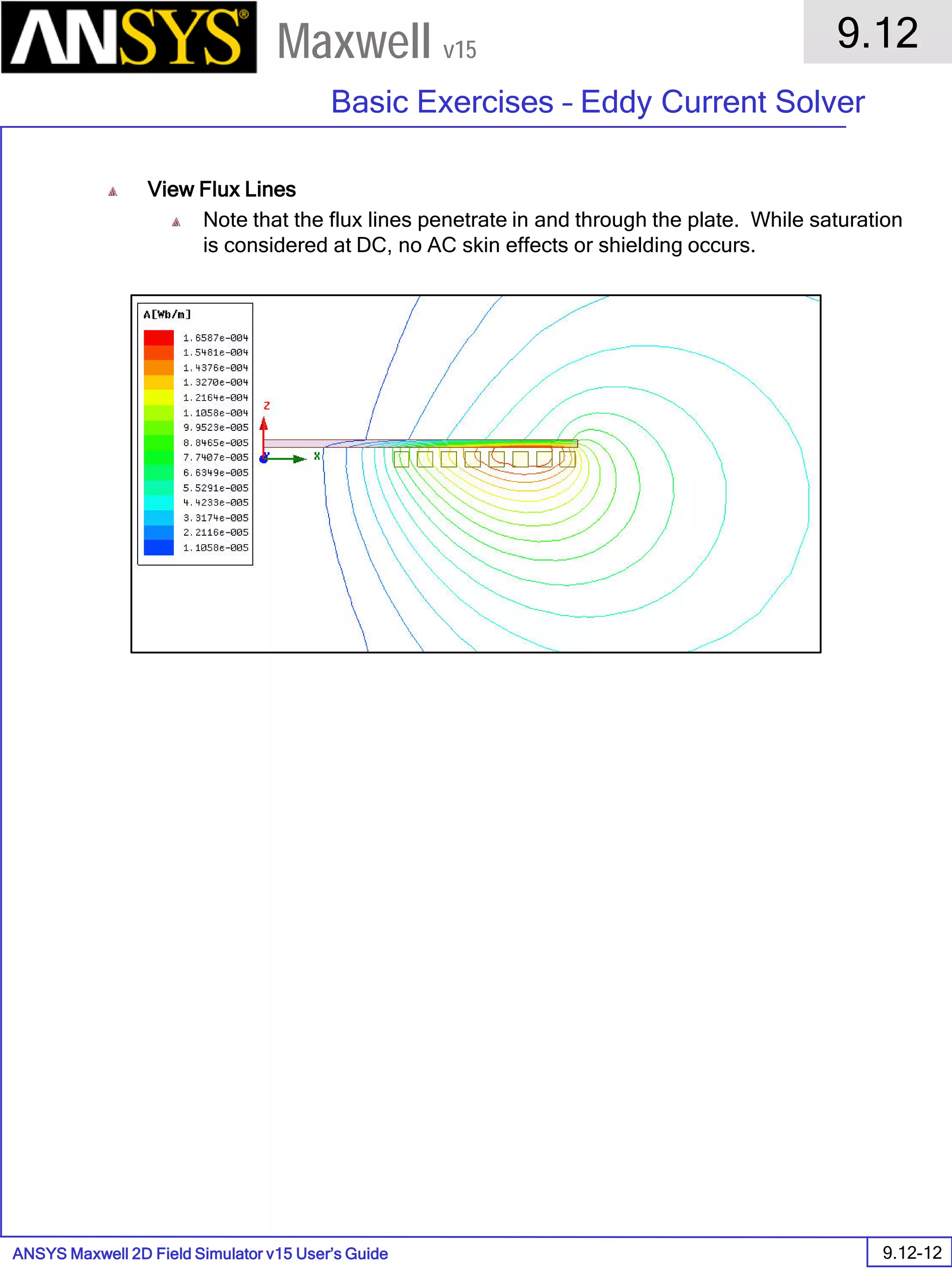
Basic Exercises – Eddy Current Solver
9.12-4
Maxwell v15
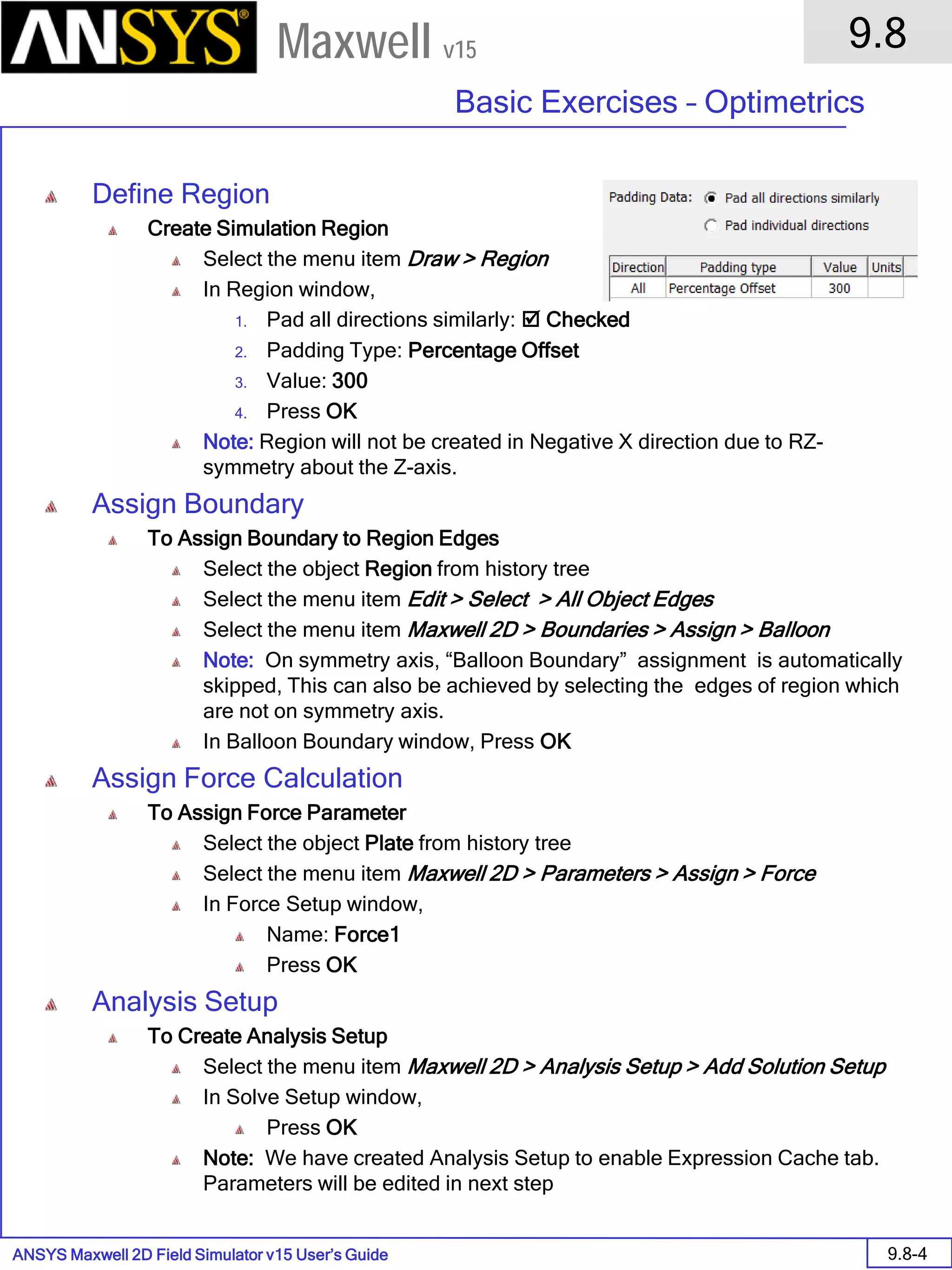
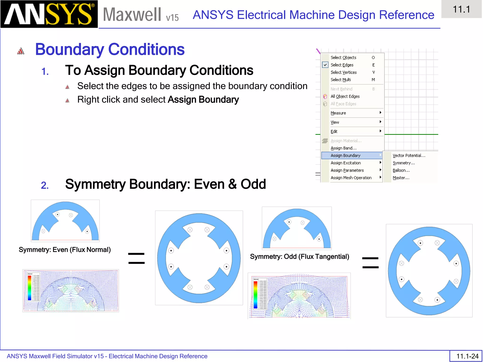
Assign Boundary
To Assign Boundary to Region Edges
Select the object Region from history tree
Select the menu item Edit > Select > All Object Edges
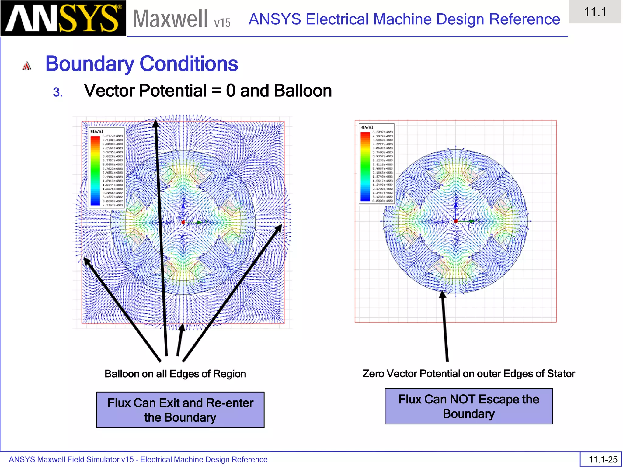
Select the menu item Maxwell 2D > Boundaries > Assign > Balloon
Note: On symmetry axis, “Balloon Boundary” assignment is automatically
skipped, This can also be achieved by selecting the edges of region which
are not on symmetry axis.
In Balloon Boundary window,
Press OK
Assign Matrix Parameters
In this example, the compete [8x8] impedance matrix will be calculated. This is
done by setting a parameter.
To Calculate Impedance Matrix
Select the menu item Maxwell 2D > Parameters > Assign > Matrix
In Matrix window,
For all current Sources
Include: Checked
Press OK
Compute the Skin Depth
Skin depth is a measure of how current density concentrates at the surface of a
conductor carrying an alternating current. It is a function of the permeability,
conductivity and frequency
Skin depth in meters is defined as follows:
where:
ω is the angular frequency, which is equal to 2πf. (f is the source frequency which in this
case is 500Hz).
σ is the conductor’s conductivity; for cast iron its 1.5e6 S/m
µr is the conductor’s relative permeability; for cast iron its 60
µο is the permeability of free space, which is equal to 4π×10-7 A/m.
For cast iron the plate the skin depth is approximately 0.24 cm.
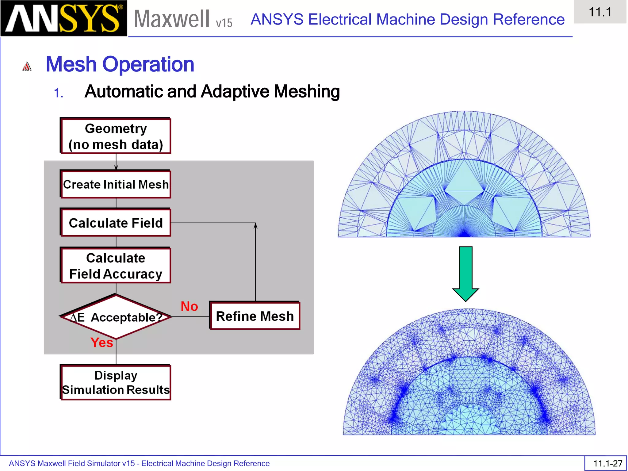
After three skin depths, the induced current will become almost negligible. The
automatic adaptive meshing in Maxwell 2D does an excellent job of refining the
mesh in the skin depth, so that mesh operations are not needed.
σµωµ
δ
ro
2
=](https://image.slidesharecdn.com/completemaxwell2dv15-160410143735/75/Complete-maxwell-2d-v15-Latest-Version-297-2048.jpg)
![ANSYS Maxwell 2D Field Simulator v15 User’s Guide
9.12
Basic Exercises – Eddy Current Solver
9.12-6
Maxwell v15
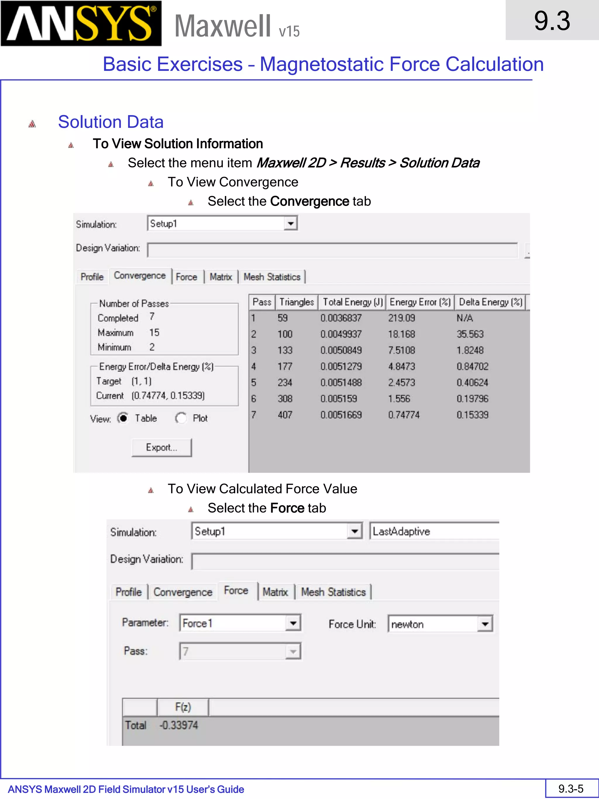
Solution Data
To View Solution Information
Select the menu item Maxwell 2D > Results > Solution Data
To view Convergence
Select the Convergence tab
To View Impedance matrix
Select Matrix tab
By default, the results are displayed as [R, Z] but can be also
shown as [R, L] or as coupling coefficients.](https://image.slidesharecdn.com/completemaxwell2dv15-160410143735/75/Complete-maxwell-2d-v15-Latest-Version-299-2048.jpg)


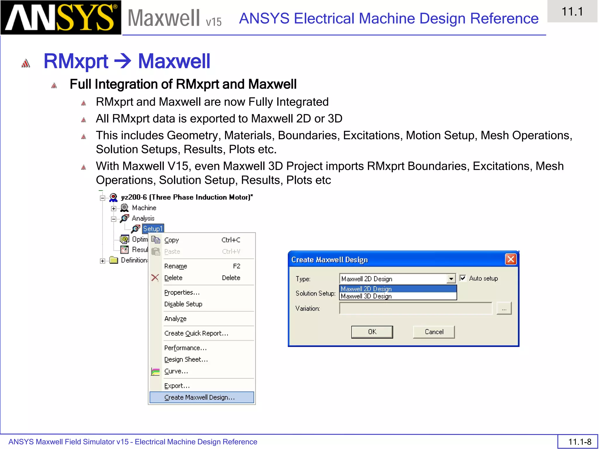
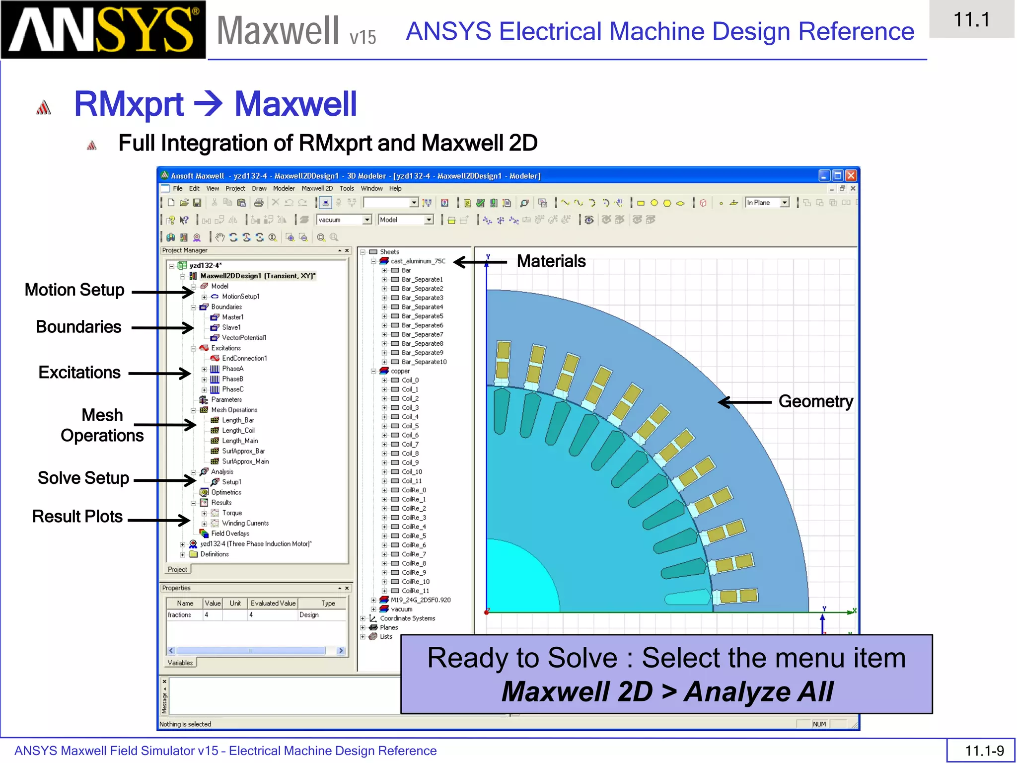
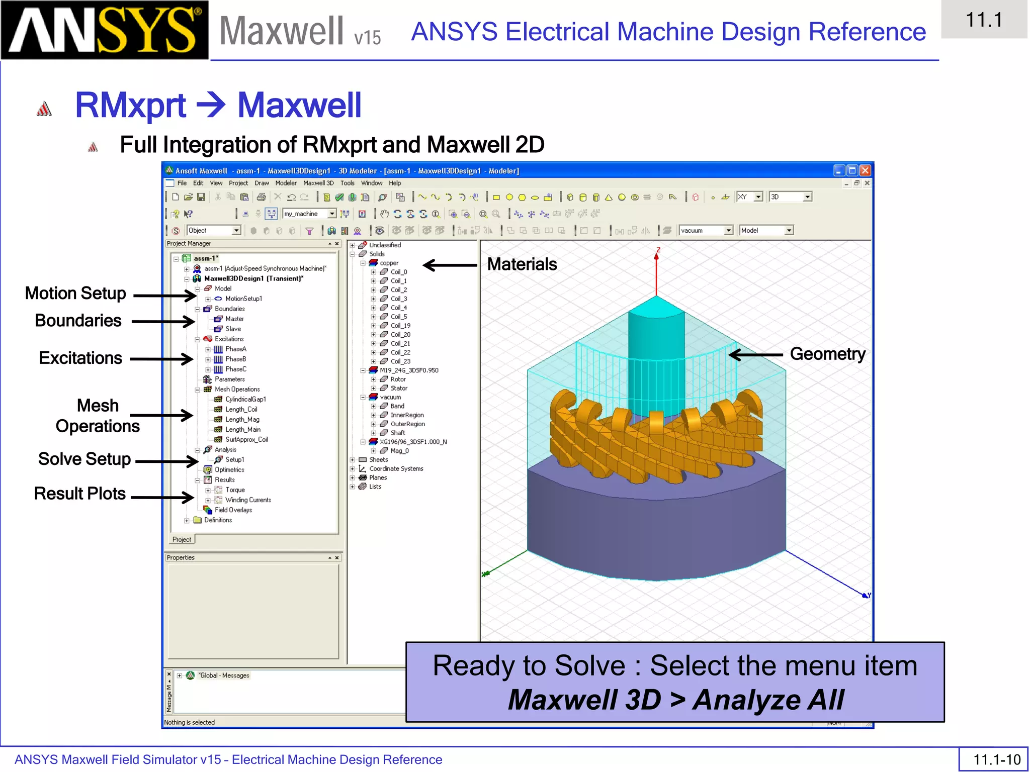


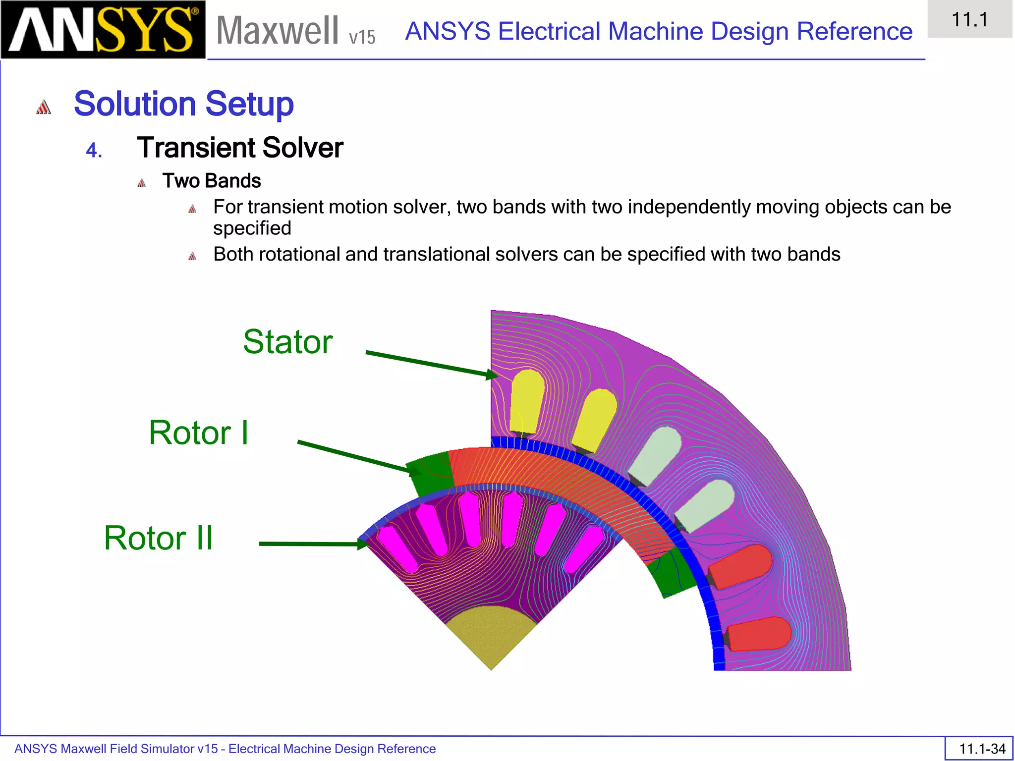
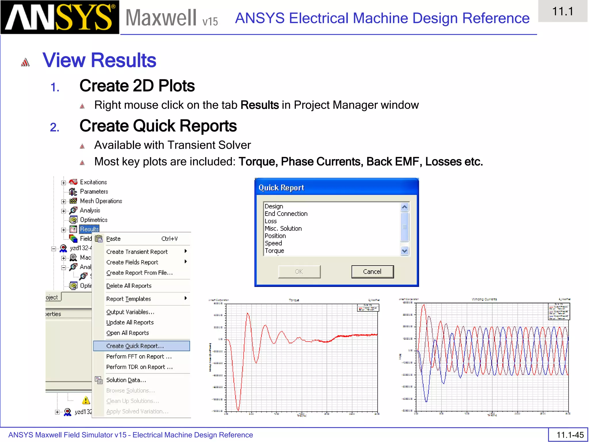
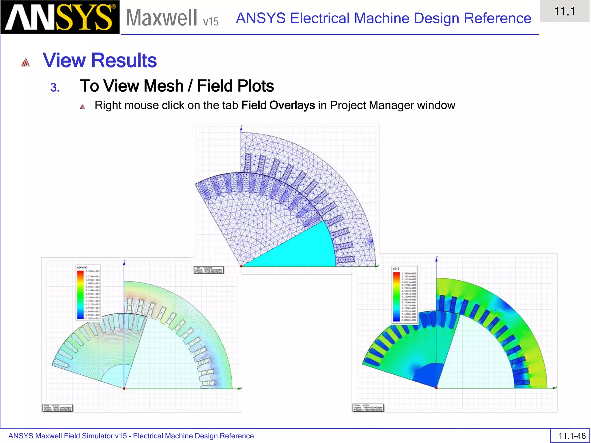
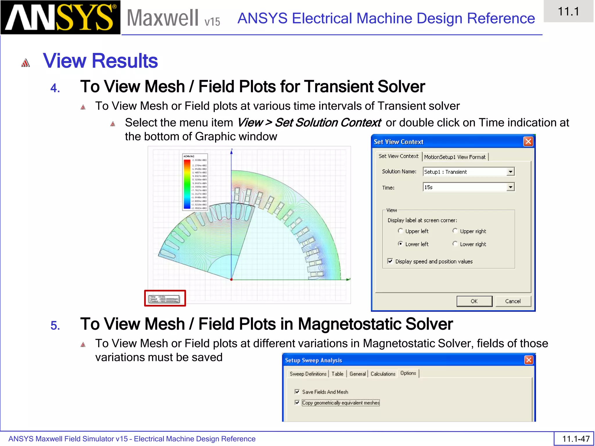
![ANSYS Maxwell Field Simulator v15 – Electrical Machine Design Reference 11.1-36
ANSYS Electrical Machine Design Reference
11.1
Maxwell v15
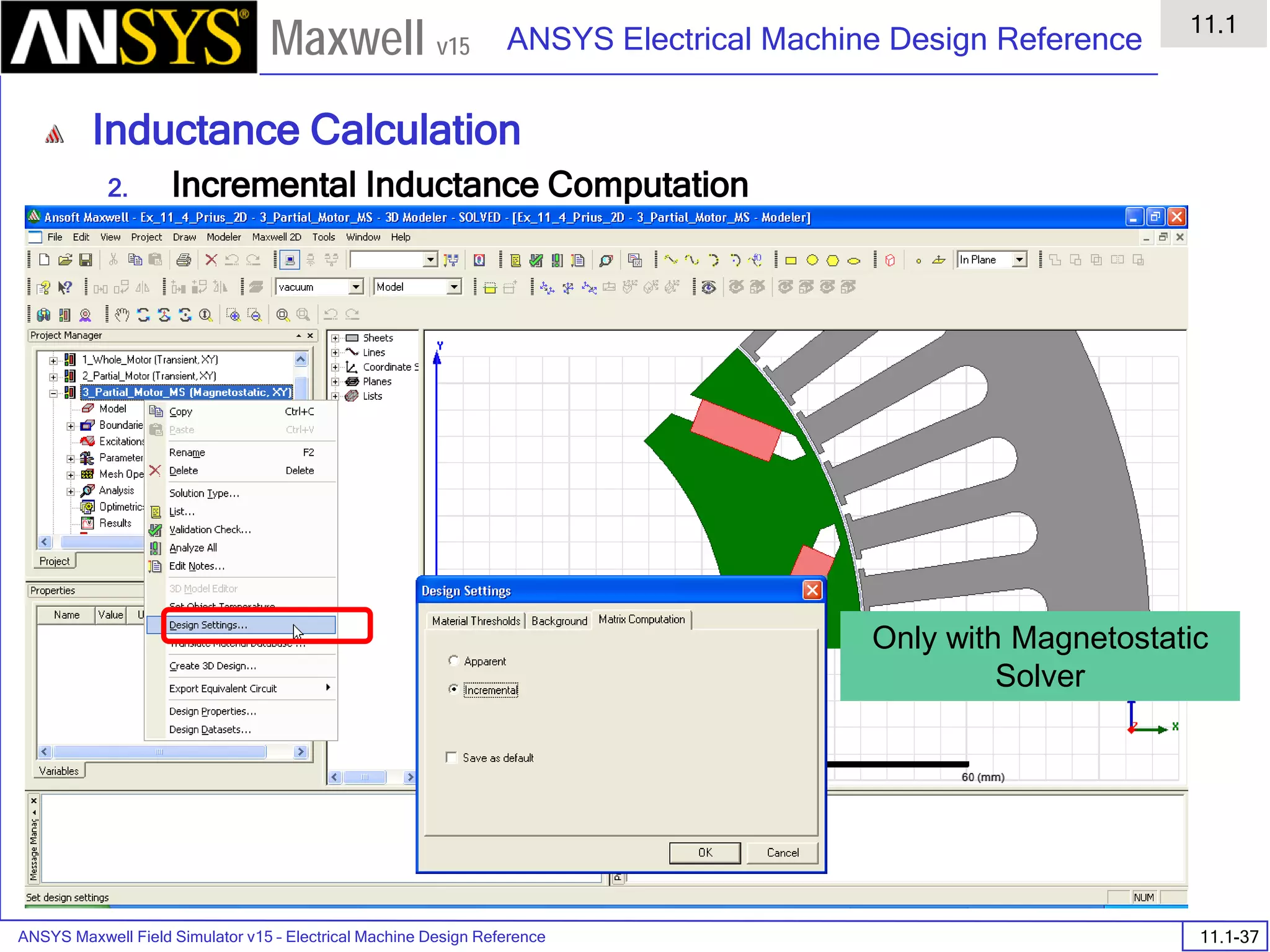
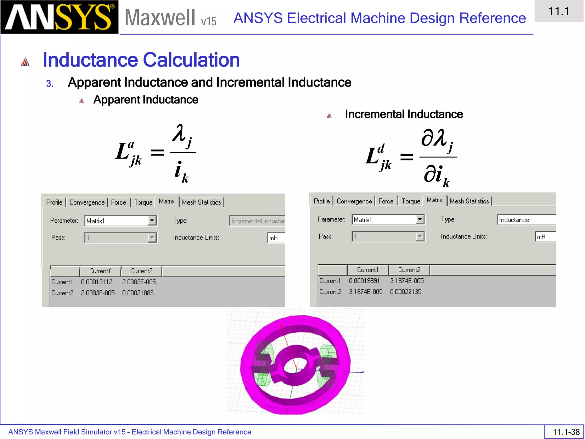
Inductance Calculation
1. Inductance Calculations with Transient Solver
100.00 200.00 300.00 400.00 500.00 600.00 700.00 800.00 900.00 1000.00
Time [us]
2.40
2.60
2.80
3.00
3.20
3.40
3.60
3.80
L(PhaseA,PhaseA)[mH]
3ph_ind_tr6XY Plot 3 ANSOFT
Curve Info
L(PhaseA,PhaseA)
Setup1 : Transient](https://image.slidesharecdn.com/completemaxwell2dv15-160410143735/75/Complete-maxwell-2d-v15-Latest-Version-394-2048.jpg)