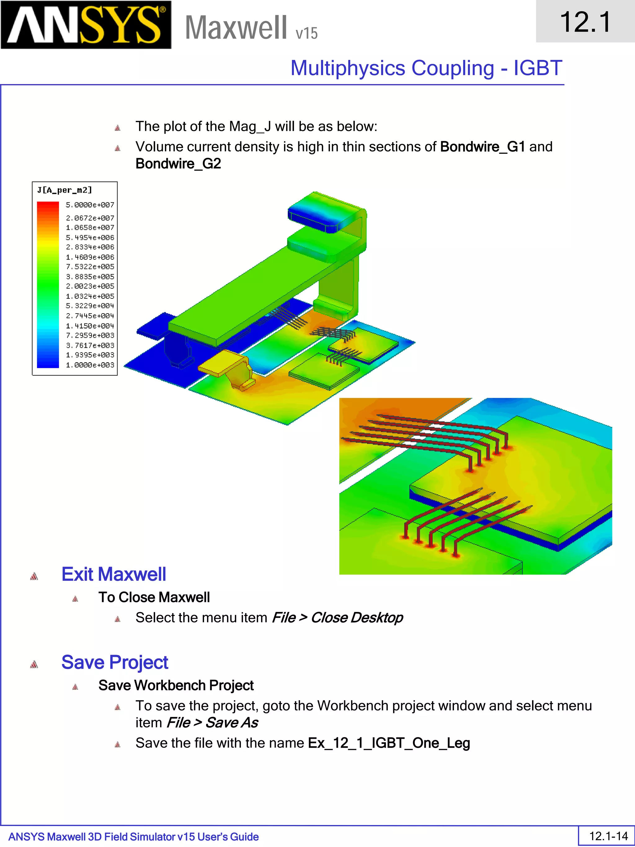
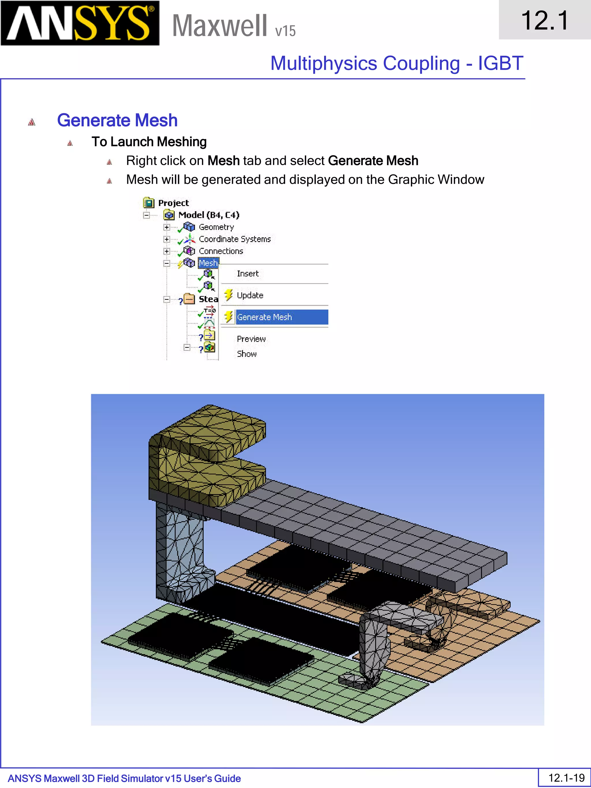
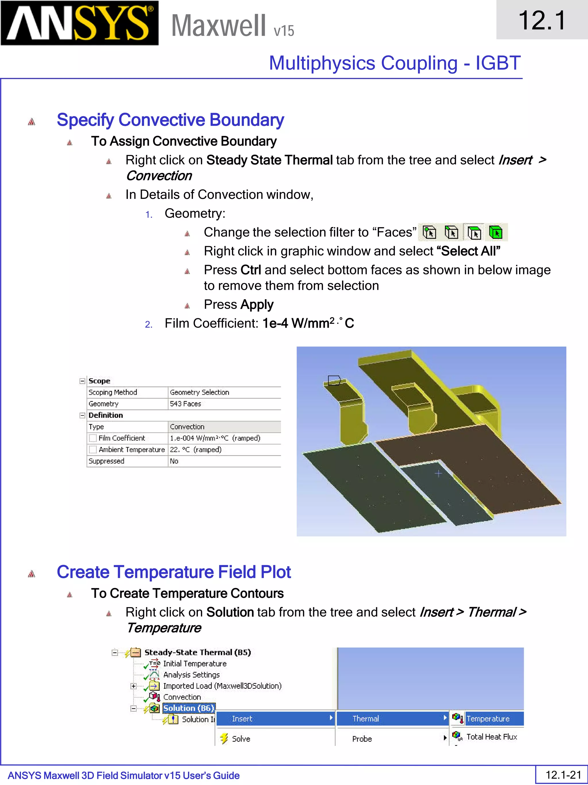
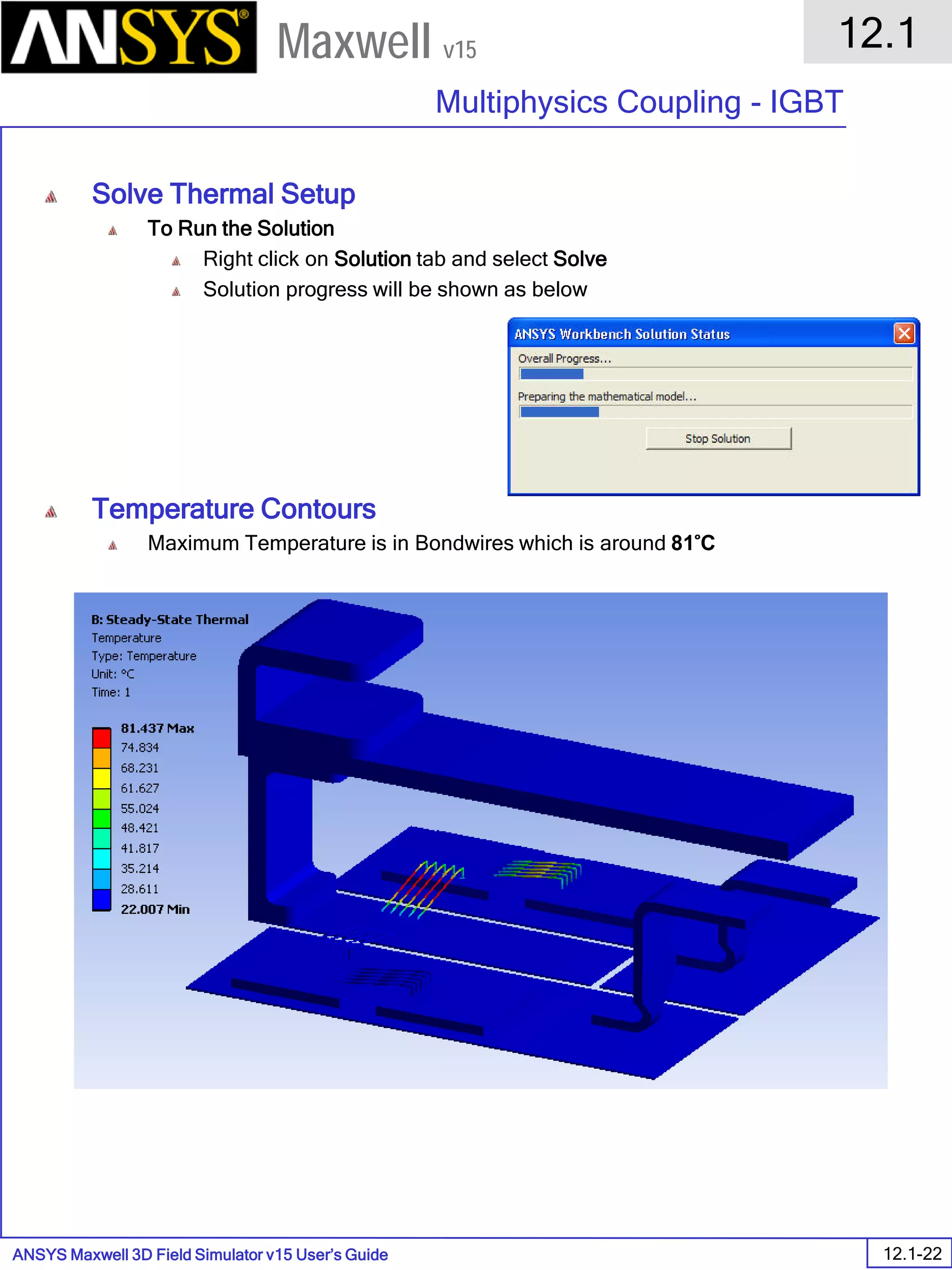
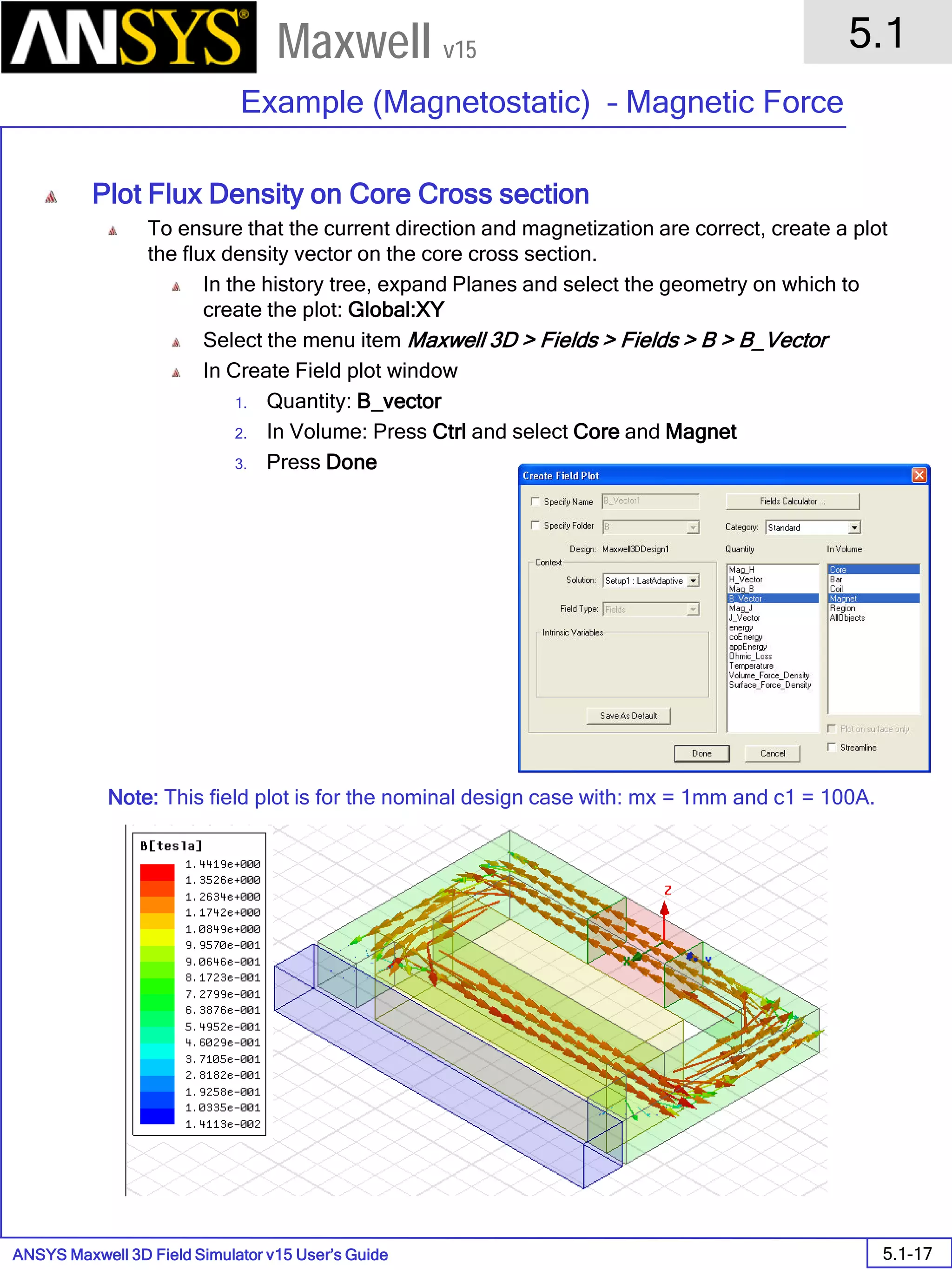
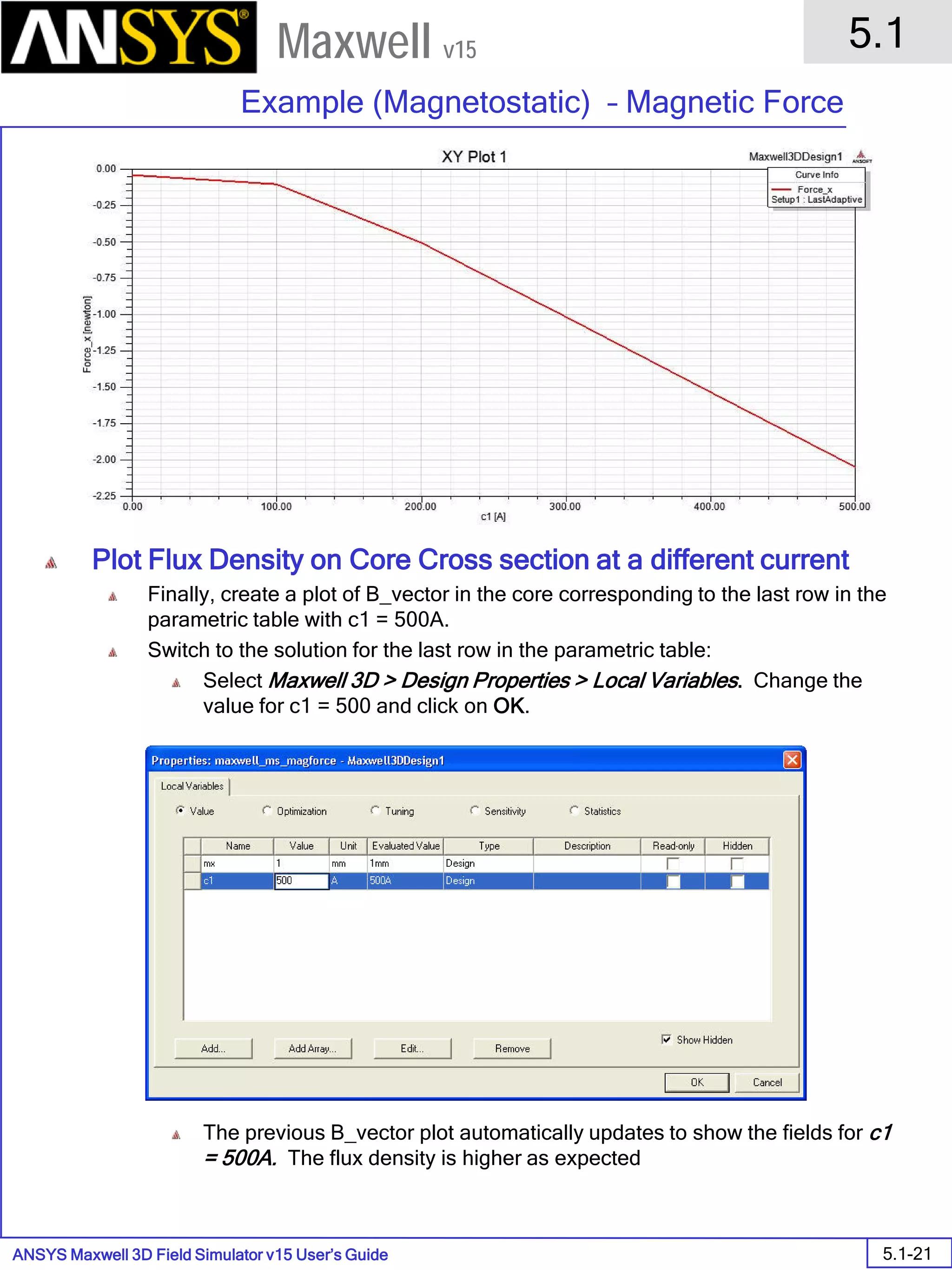
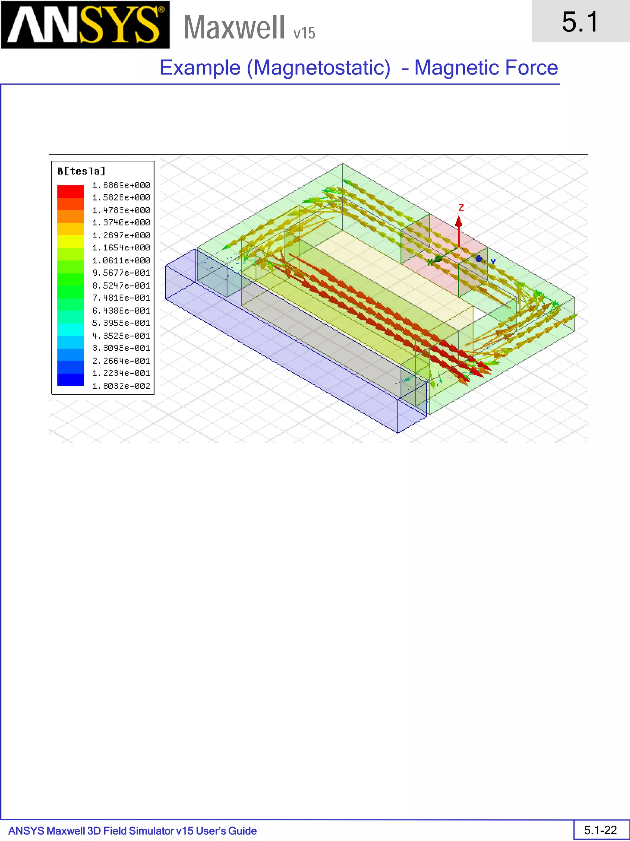
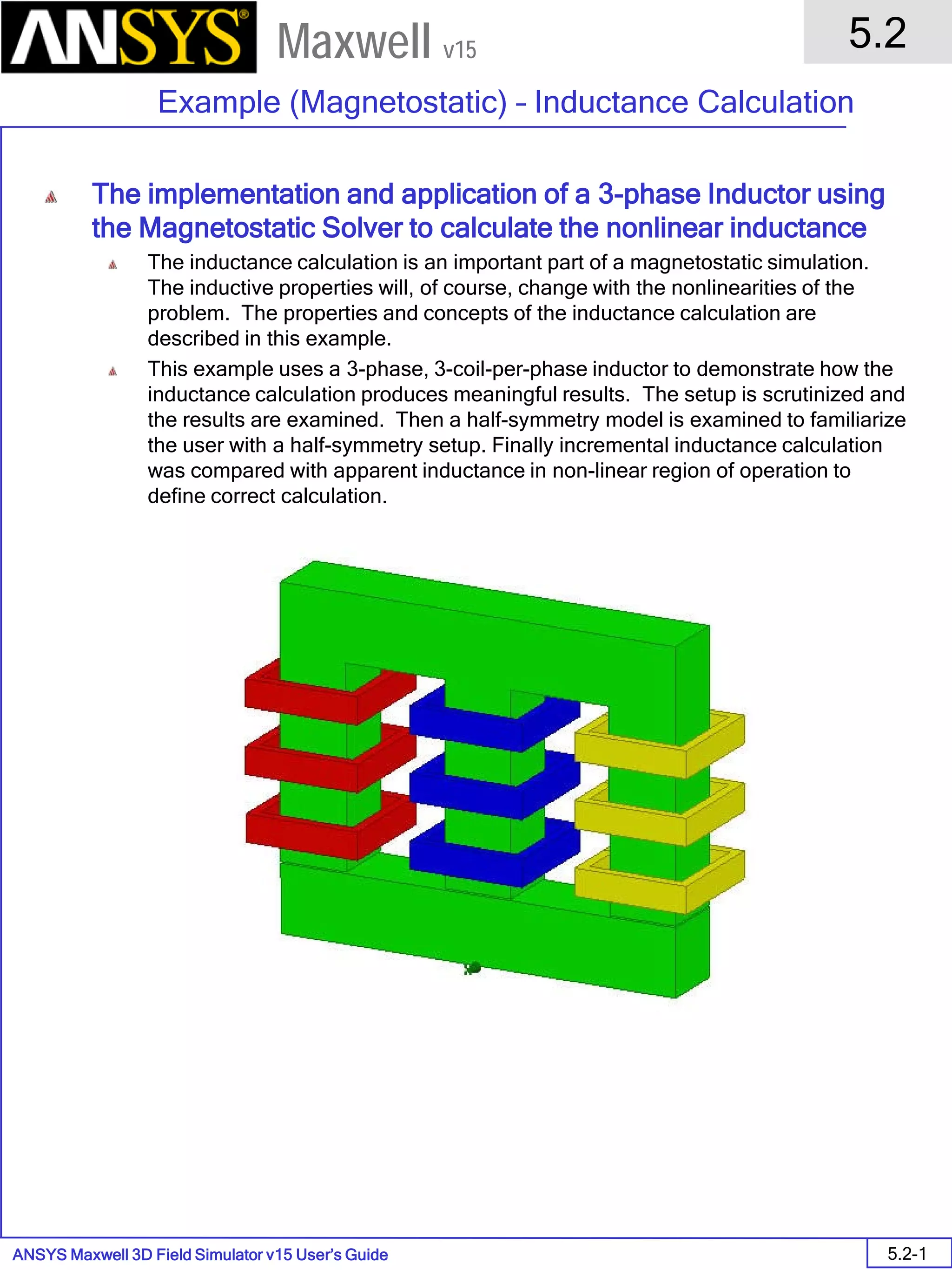
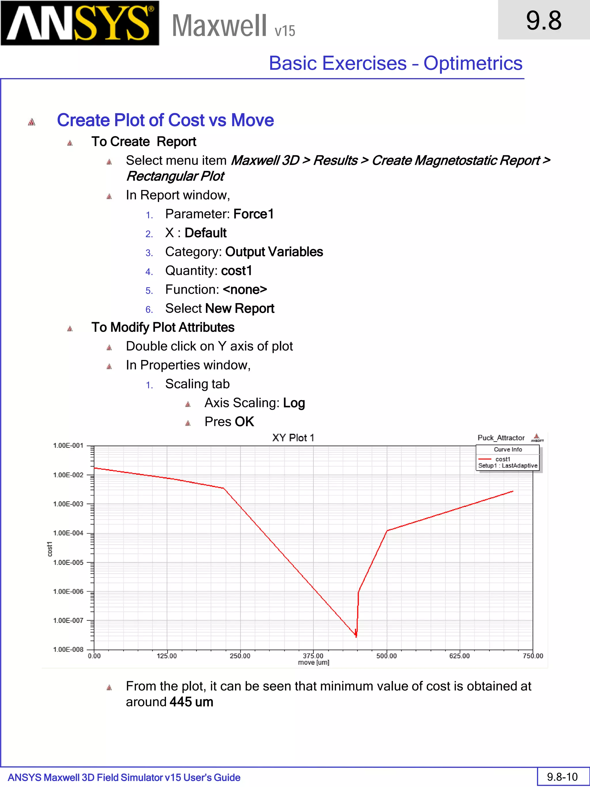
This document provides an overview and user's guide for the Maxwell 3D electromagnetic simulation software. It discusses the solution types, meshing process, data reporting, and provides examples for magnetostatic, eddy current, transient, electric, and multiphysics analyses. The guide covers the Maxwell interface, modeling capabilities including importing CAD files, meshing, solving Maxwell's equations, and post-processing of results. It is intended to help new users understand the basic concepts and functionality of the Maxwell software.


![ANSYS Maxwell Field Simulator v15 – Training Seminar P1-39
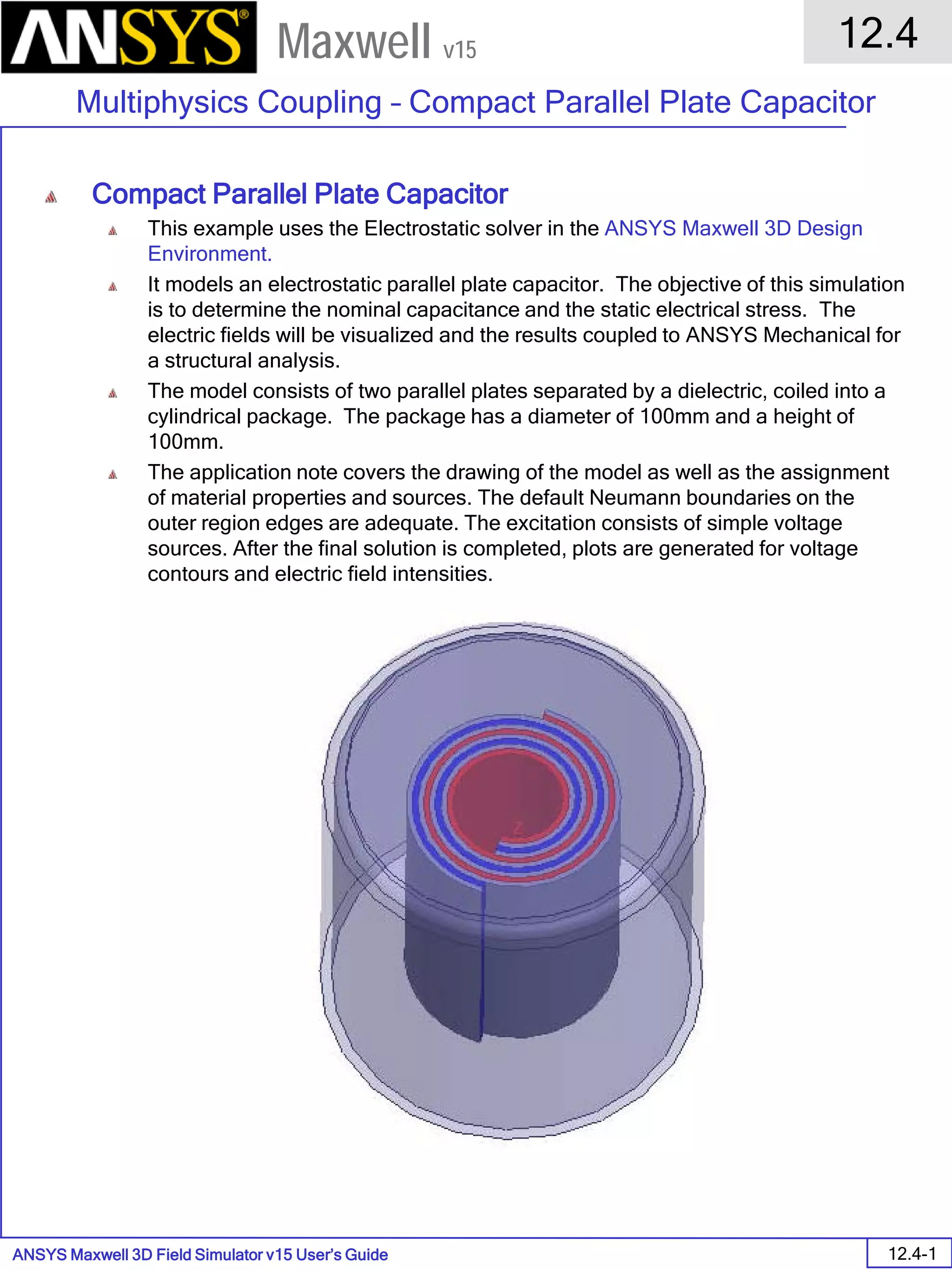
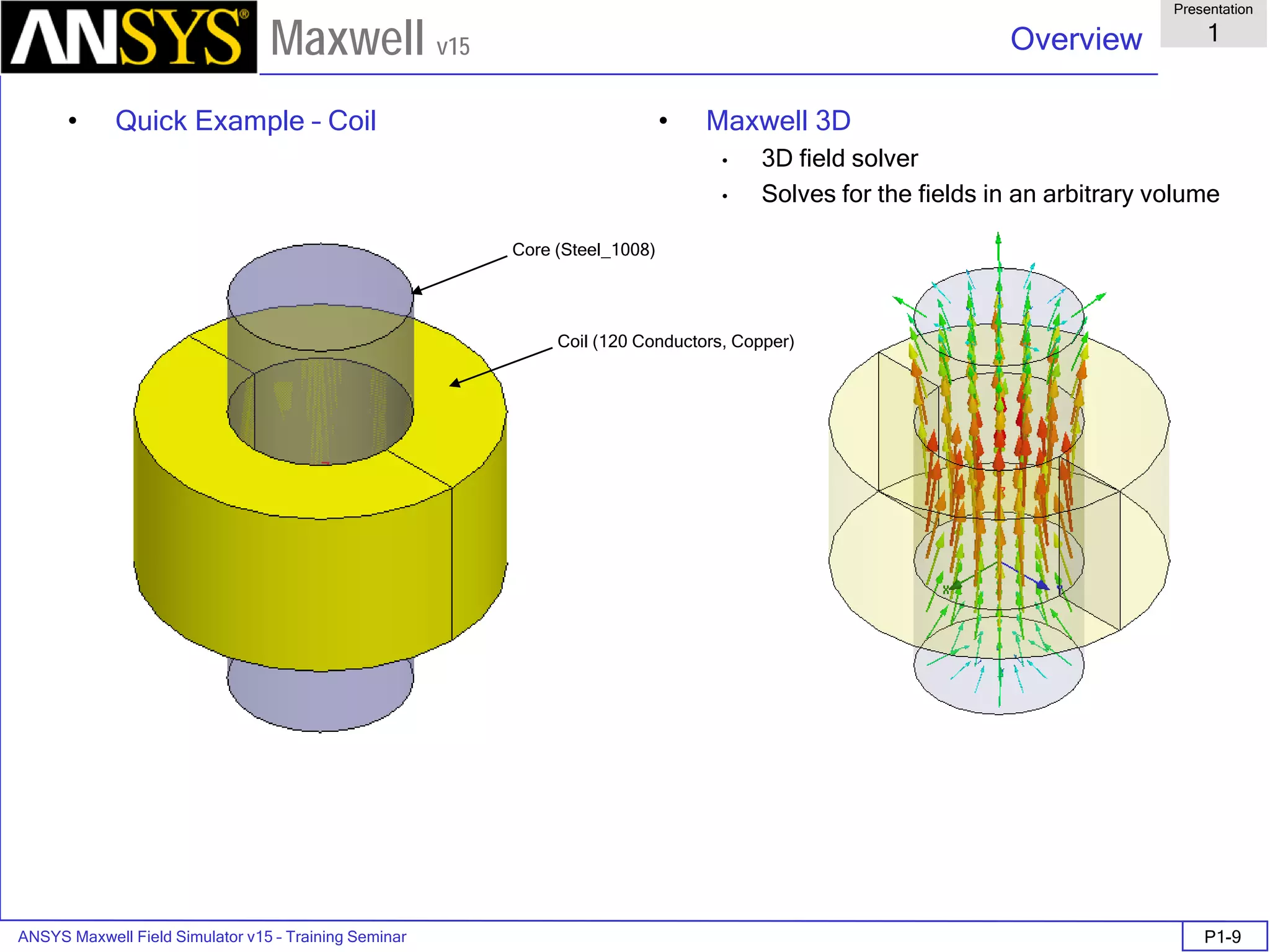
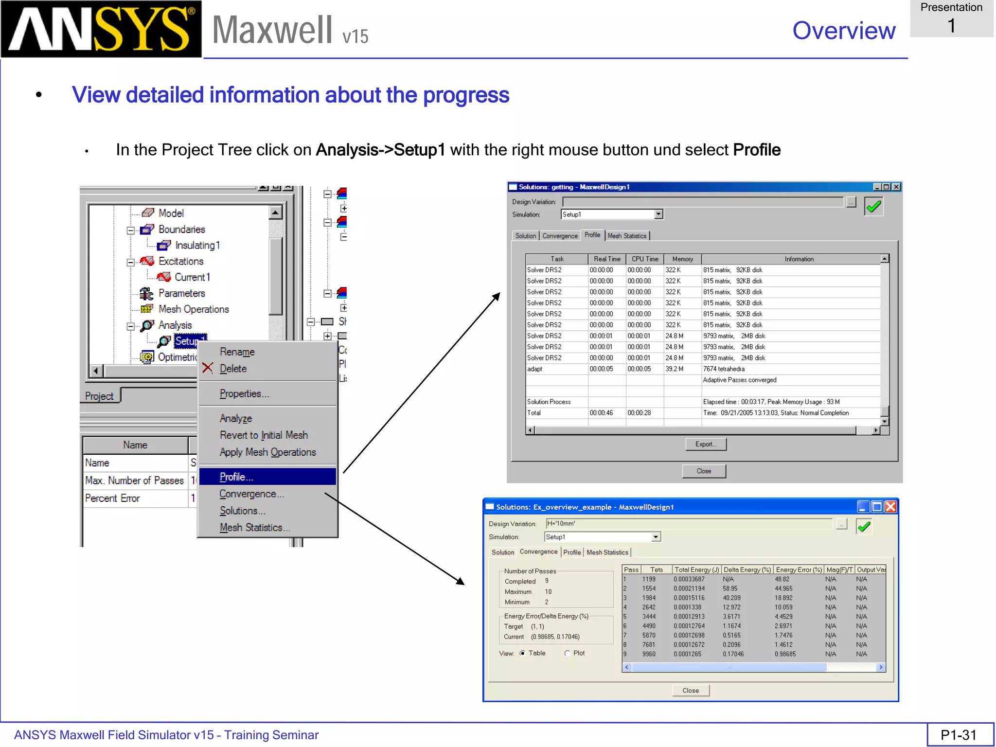
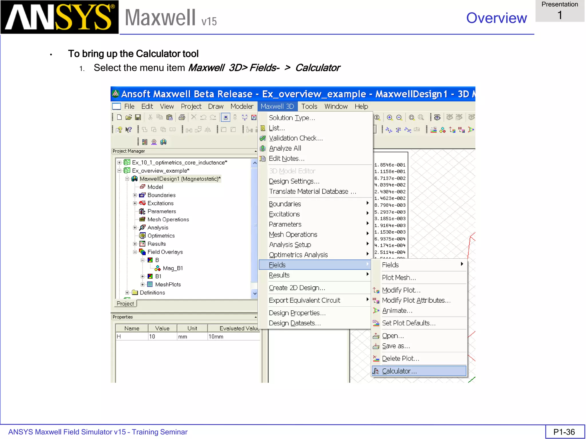
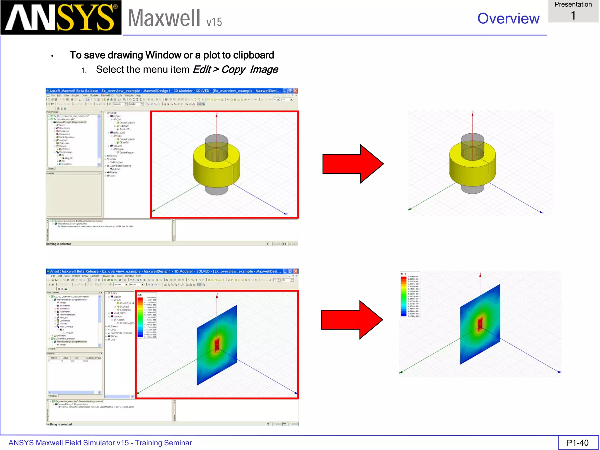
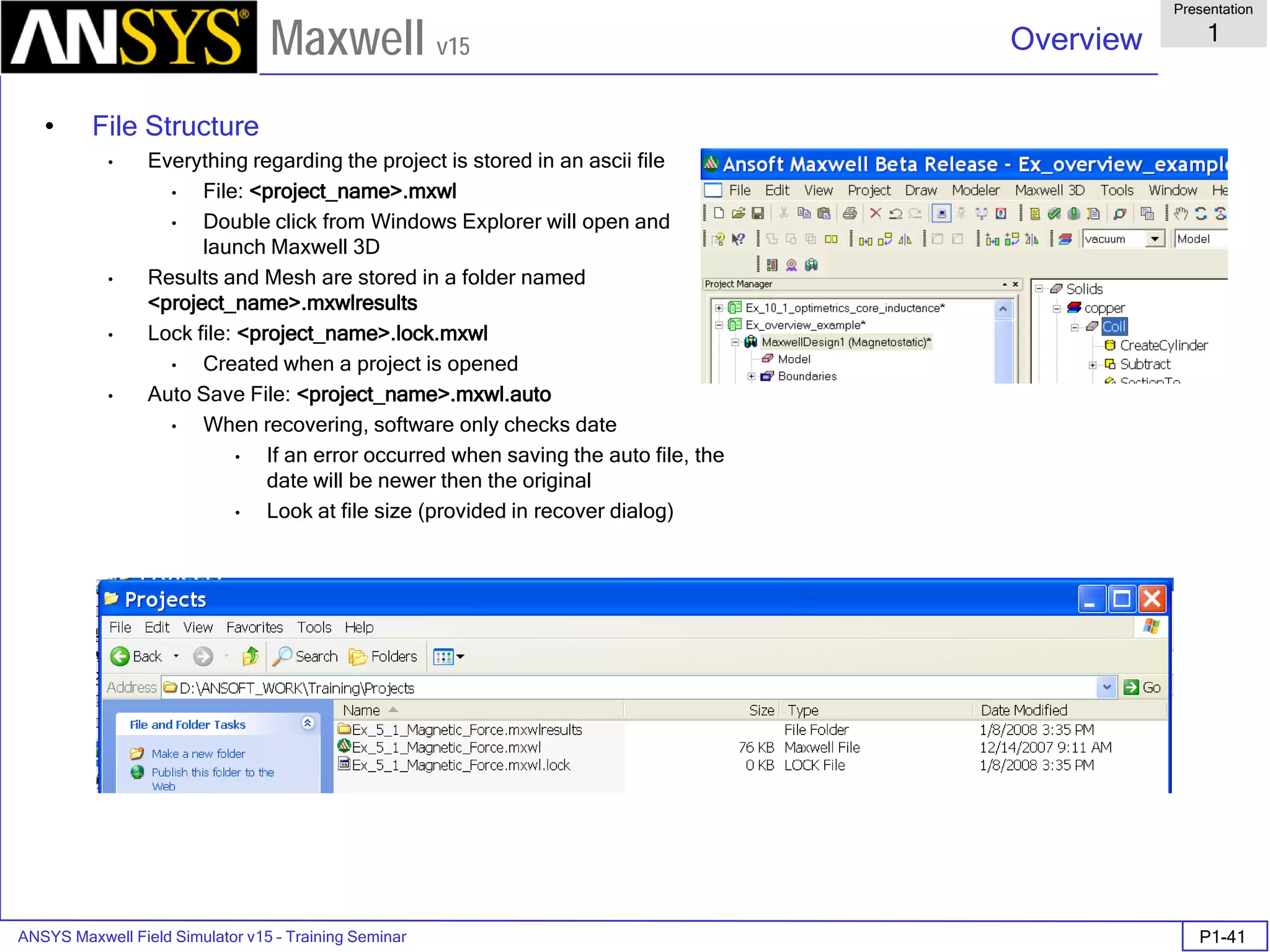
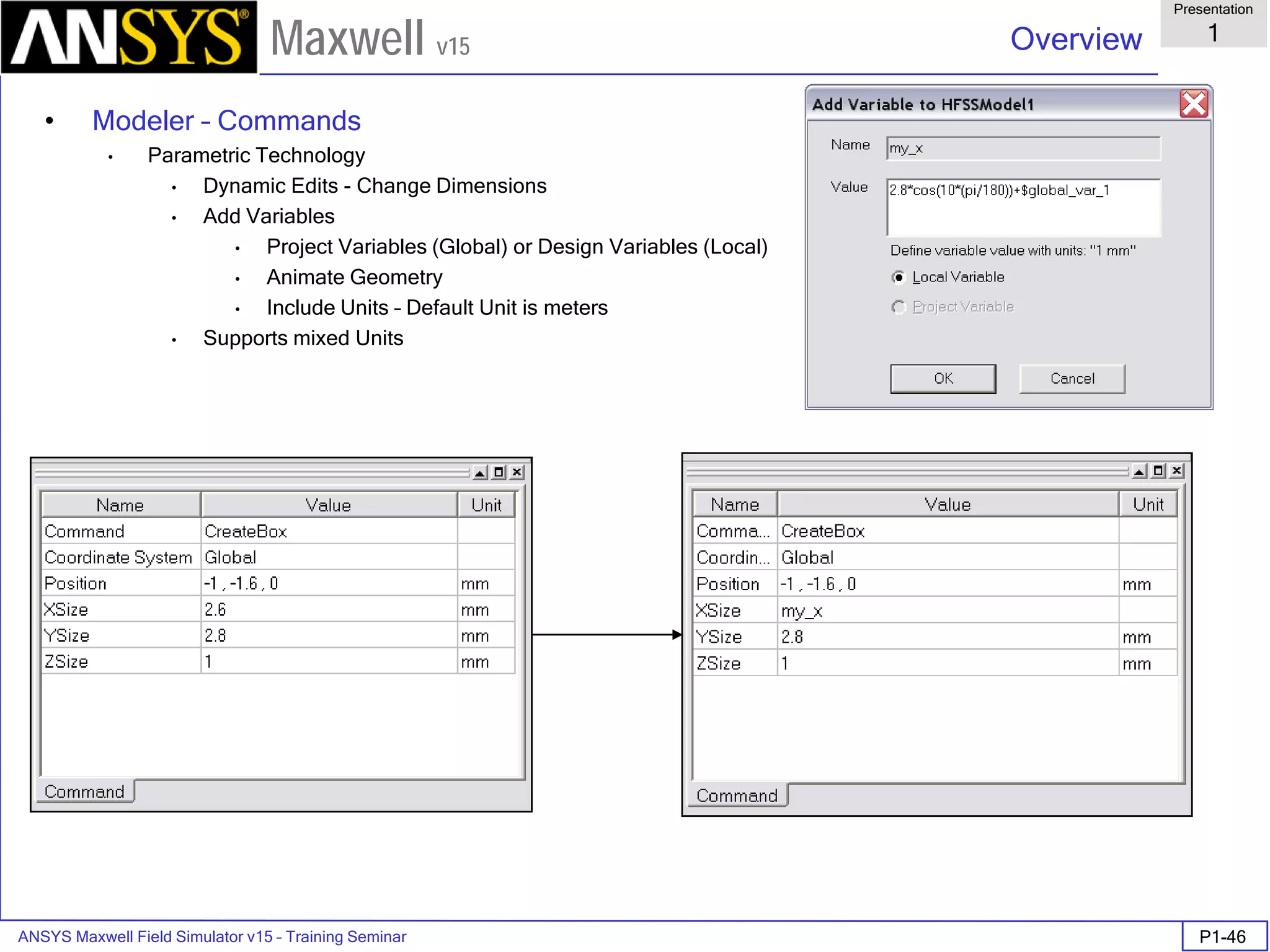
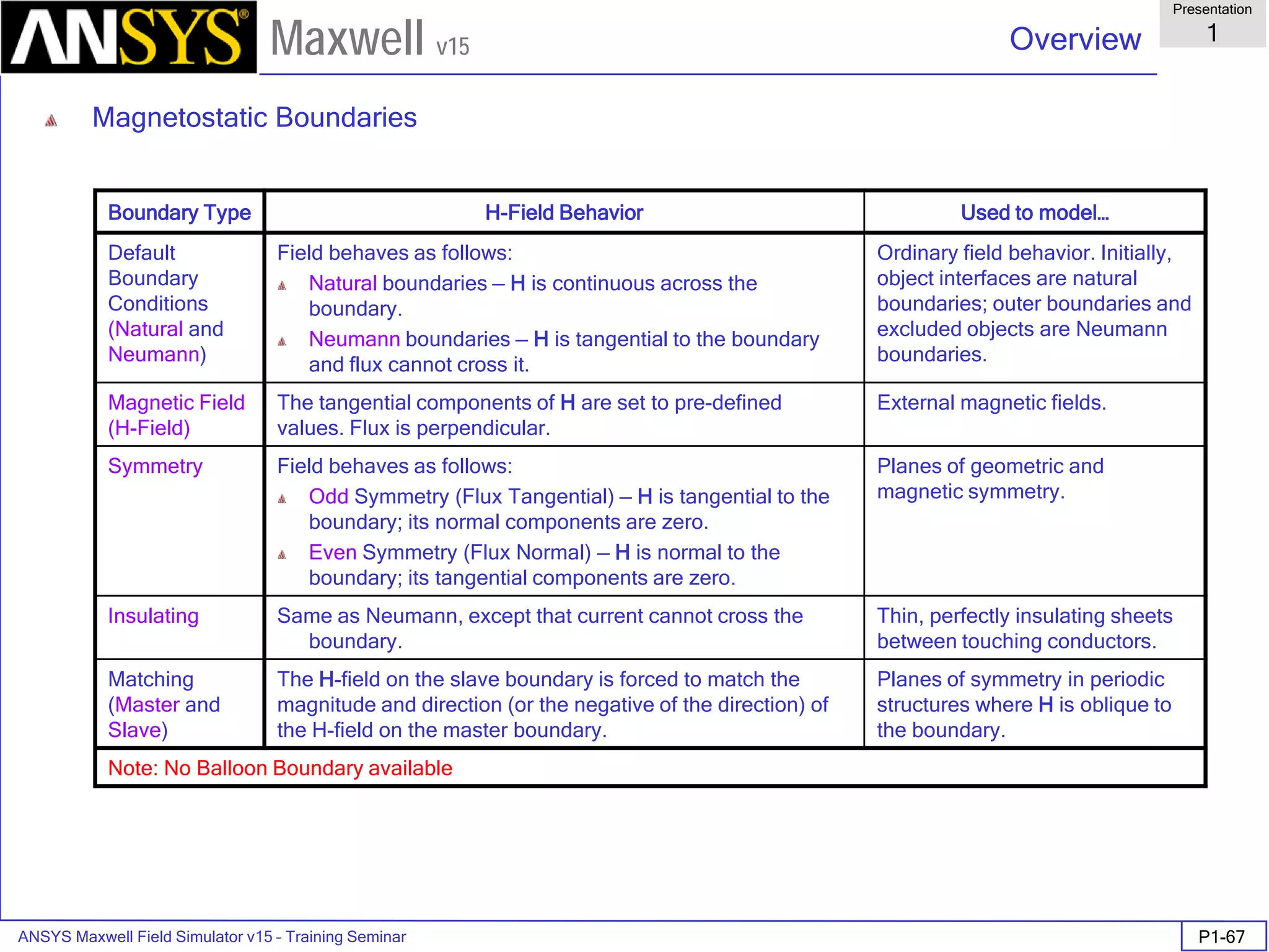
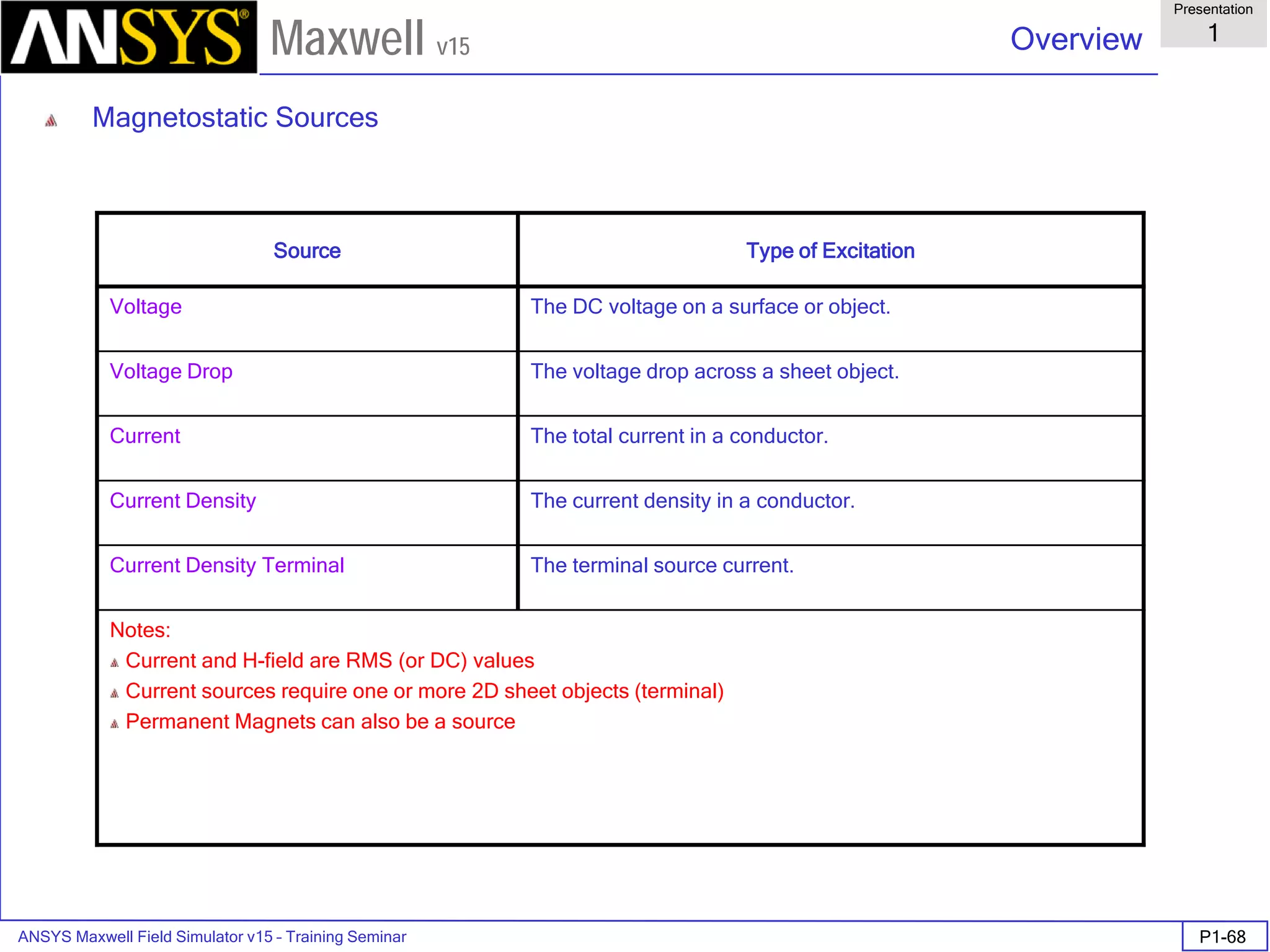
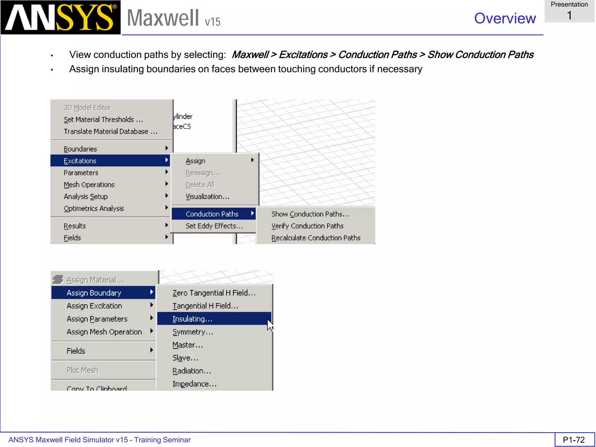
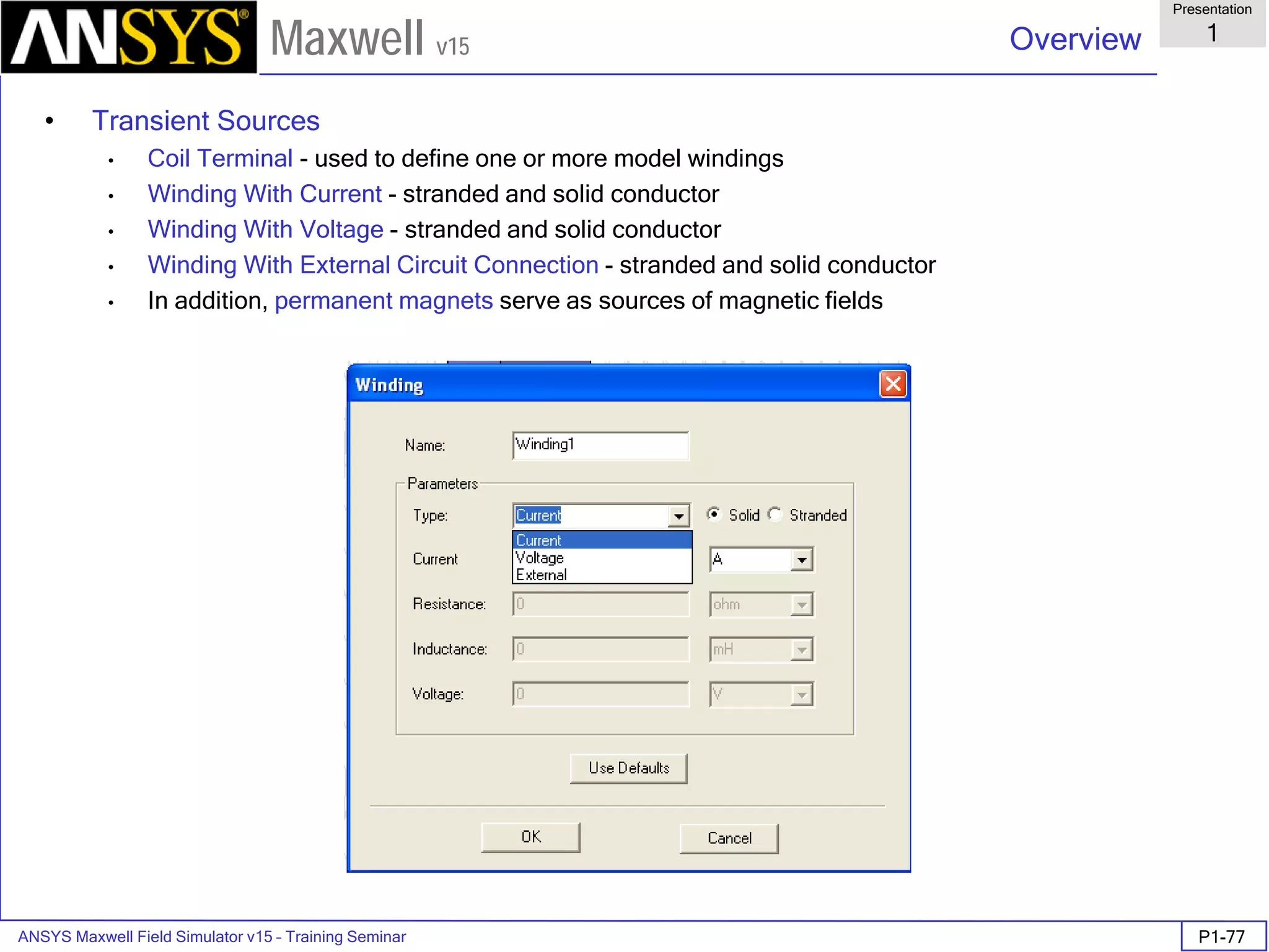
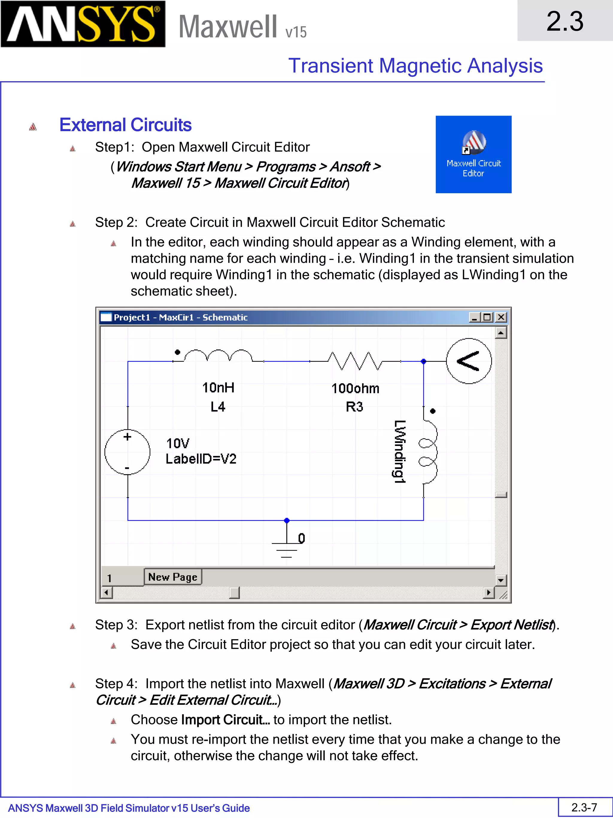
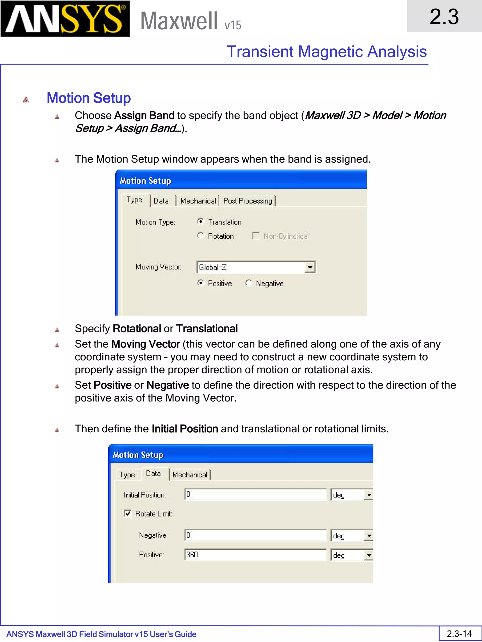
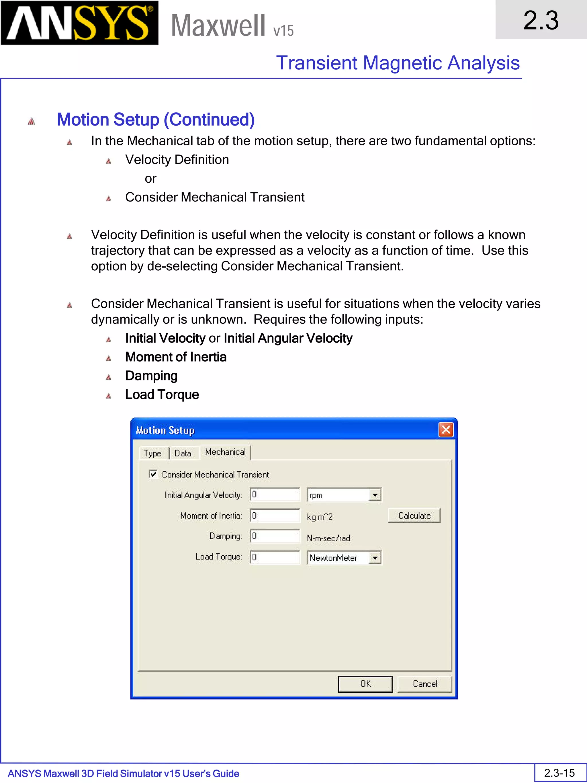
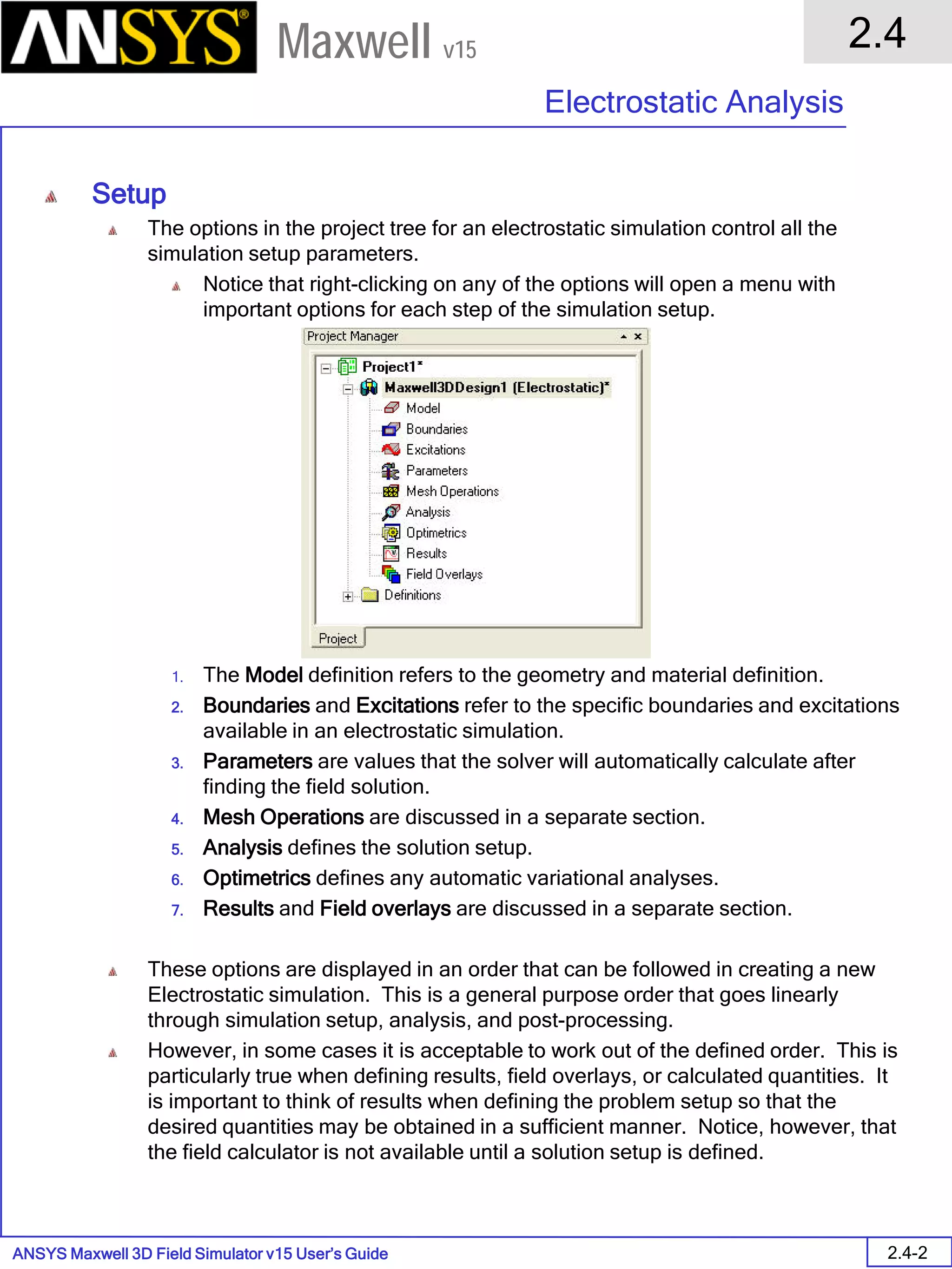
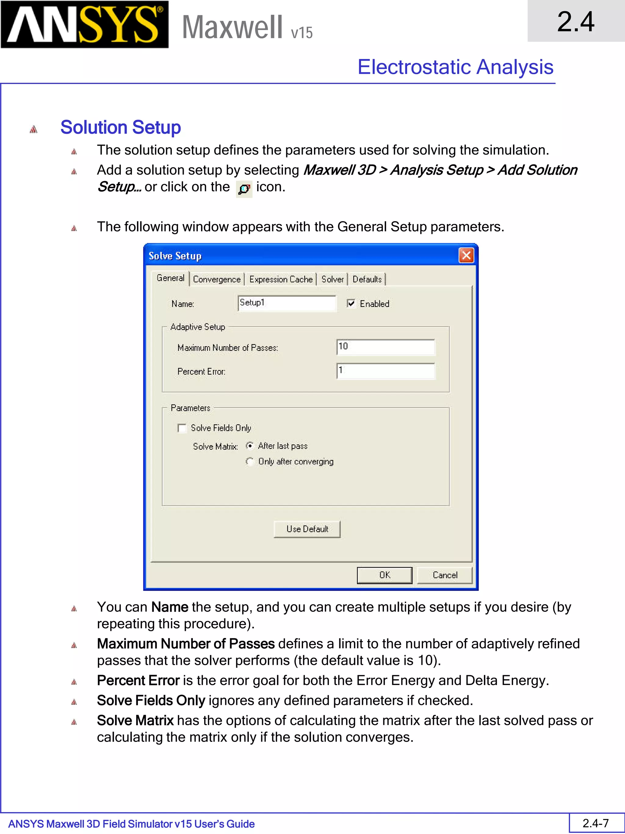
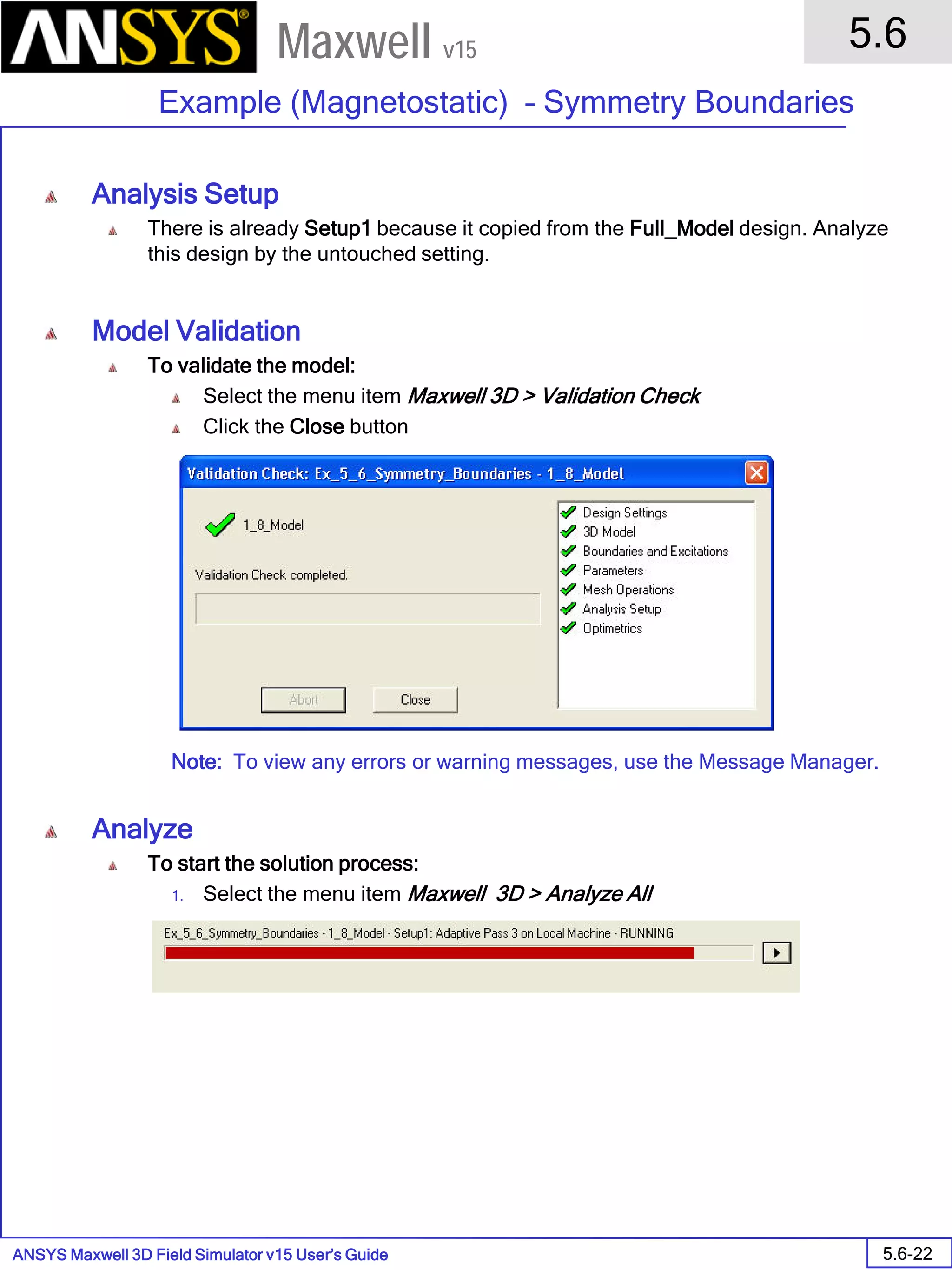
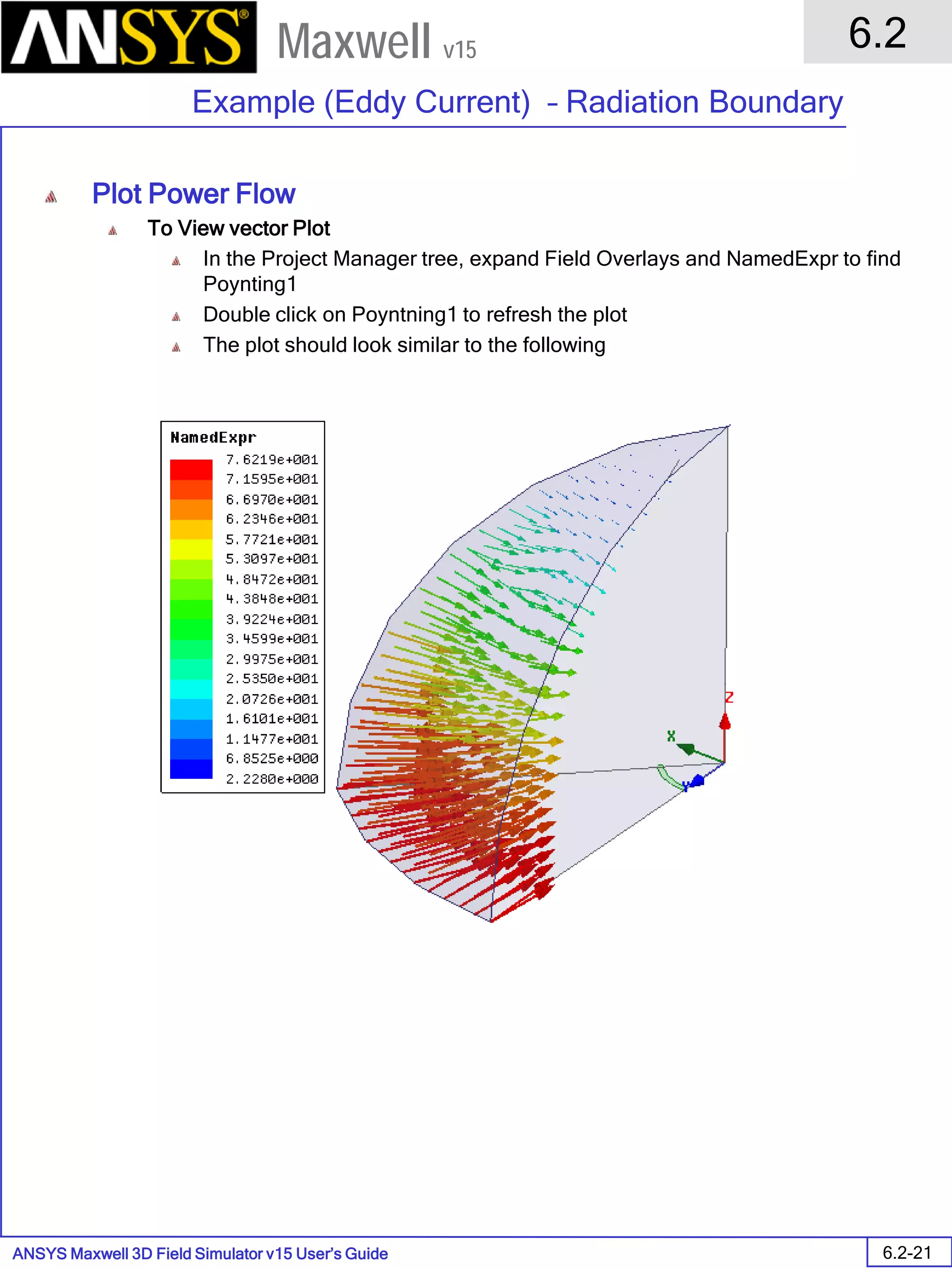
Overview
Presentation
1
Maxwell v15
0.00 5.00 10.00 15.00 20.00
Distance [mm]
0.000
0.005
0.010
0.015
0.020
0.025
0.030
Bz
Ansoft Corporation MaxwellDesign1XY Plot 1
Curve Info
Bz
Setup1 : LastAdaptive](https://image.slidesharecdn.com/maxwell3d-160822035138/75/Maxwell3-d-43-2048.jpg)


![ANSYS Maxwell Field Simulator v15 – Training Seminar P1-64
Overview
Presentation
1
Maxwell v15
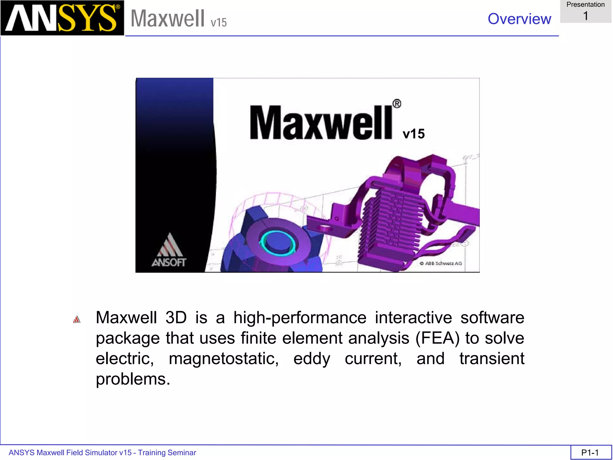
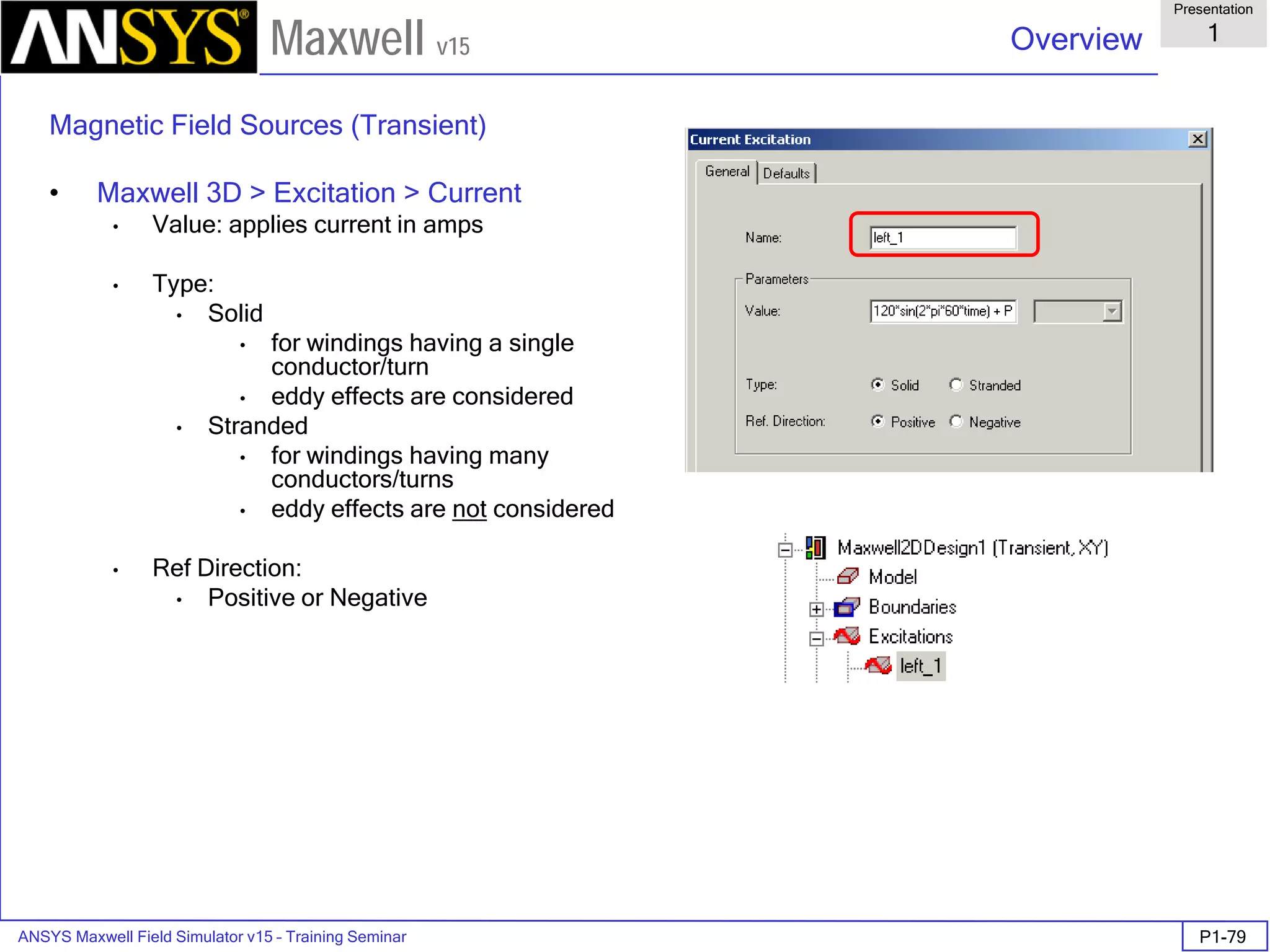
• Material setup - Anisotropic Material Properties
• ε1, µ1, and σ1 are tensors in the X direction.
• ε2, µ2, and σ2 are tensors in the Y direction.
• ε3, µ3, and σ3 are tensors in the Z direction.
• Anisotropic permeability definitions can be either LINEAR or NONLINEAR.
[ ] [ ] [ ]
Transient
&Current,Eddy
3
2
1
Transient
&Current,Eddy
tic,Magnetosta
3
2
1
CurrentEddy
&ticElectrosta
3
2
1
00
00
00
,
00
00
00
,
00
00
00
=
=
=
σ
σ
σ
σ
µ
µ
µ
µ
ε
ε
ε
ε](https://image.slidesharecdn.com/maxwell3d-160822035138/75/Maxwell3-d-68-2048.jpg)


![ANSYS Maxwell Field Simulator v15 – Training Seminar P1-107
Overview
Presentation
1
Maxwell v15
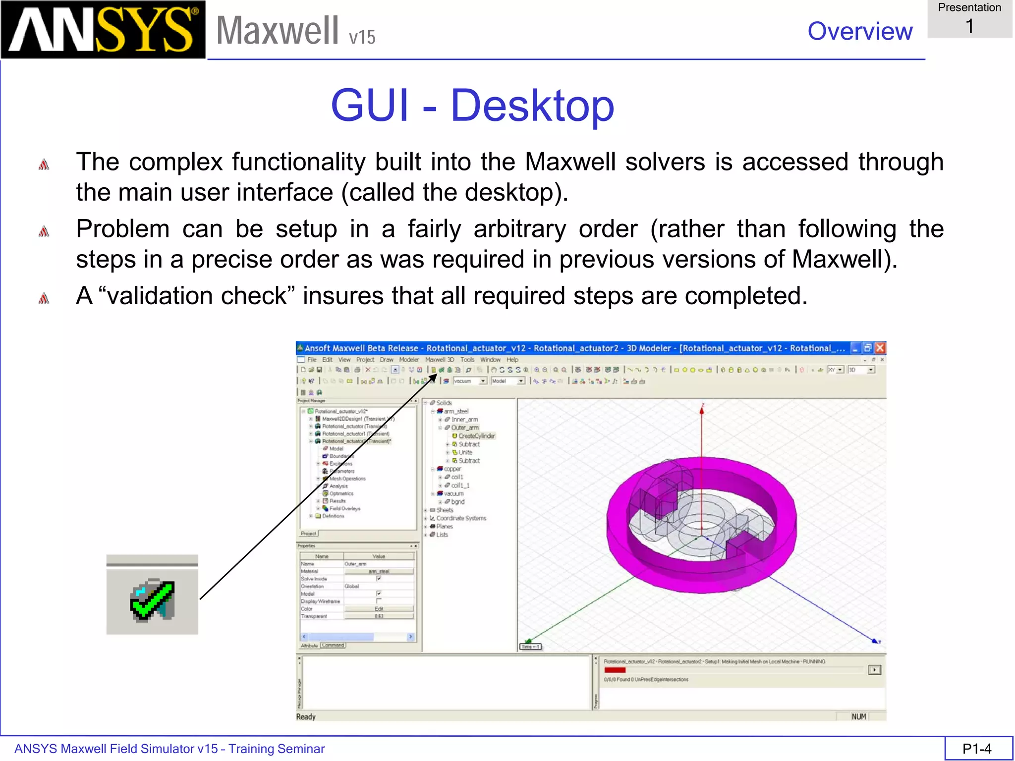
• Export to Grid
• Vector data <Ex,Ey,Ez>
• Min: [0 0 0]
• Max: [2 2 2]
• Spacing: [1 1 1]
• Space delimited ASCII file saved in
project subdirectory
Vector data "<Ex,Ey,Ez>"
Grid Output Min: [0 0 0] Max: [2 2 2] Grid Size: [1 1 1
0 0 0 -71.7231 -8.07776 128.093
0 0 1 -71.3982 -1.40917 102.578
0 0 2 -65.76 -0.0539669 77.9481
0 1 0 -259.719 27.5038 117.572
0 1 1 -248.088 16.9825 93.4889
0 1 2 -236.457 6.46131 69.4059
0 2 0 -447.716 159.007 -8.6193
0 2 1 -436.085 -262.567 82.9676
0 2 2 -424.454 -236.811 58.8847
1 0 0 -8.91719 -241.276 120.392
1 0 1 -8.08368 -234.063 94.9798
1 0 2 -7.25016 -226.85 69.5673
1 1 0 -271.099 -160.493 129.203
1 1 1 -235.472 -189.125 109.571
1 1 2 -229.834 -187.77 84.9415
1 2 0 -459.095 -8.55376 2.12527
1 2 1 -447.464 -433.556 94.5987
1 2 2 -435.833 -407.8 70.5158
2 0 0 101.079 -433.897 -18.5698
2 0 1 -327.865 -426.684 95.8133
2 0 2 -290.824 -419.471 70.4008
2 1 0 -72.2234 -422.674 -9.77604
2 1 1 -495.898 -415.461 103.026
2 1 2 -458.857 -408.248 77.6138
2 2 0 -470.474 -176.115 12.8698
2 2 1 -613.582 -347.994 83.2228
2 2 2 -590.326 -339.279 63.86](https://image.slidesharecdn.com/maxwell3d-160822035138/75/Maxwell3-d-111-2048.jpg)


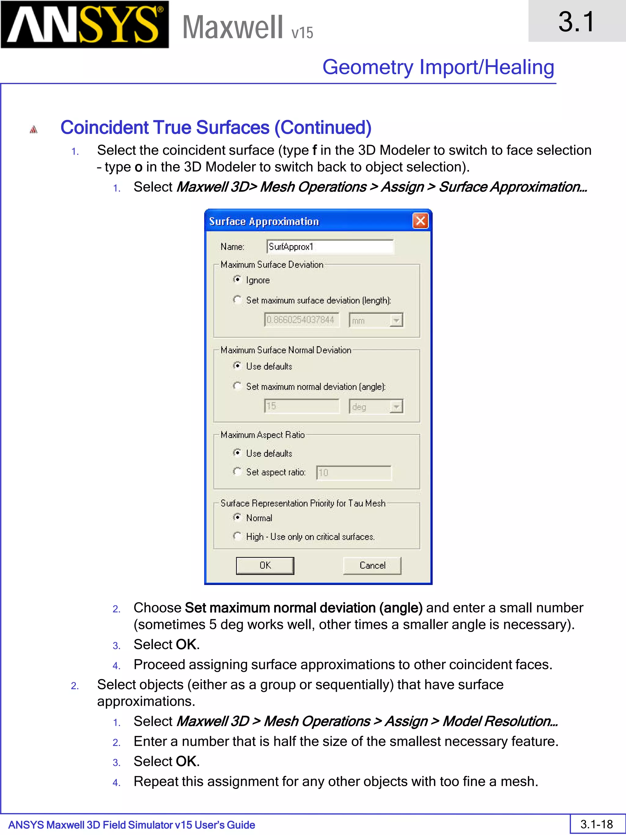
![ANSYS Maxwell 3D Field Simulator v15 User’s Guide
2.0
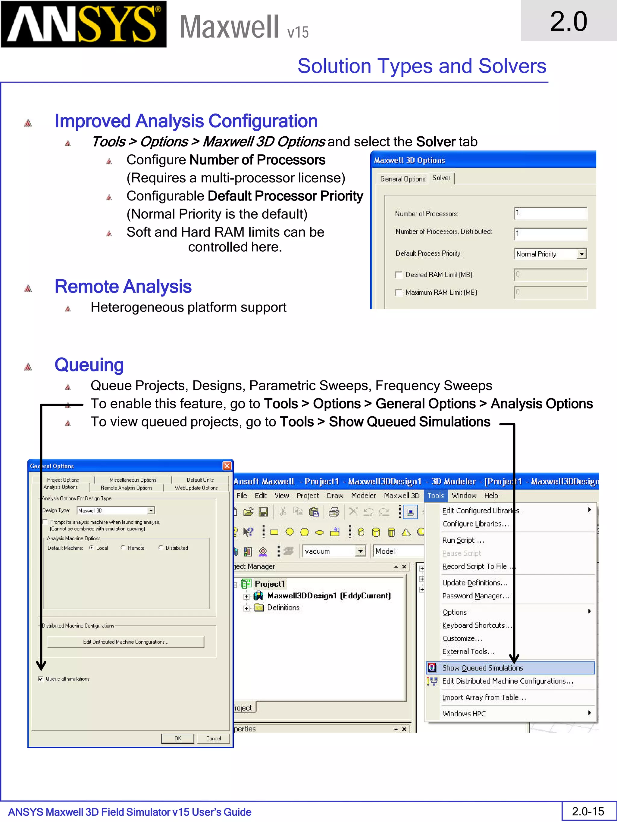
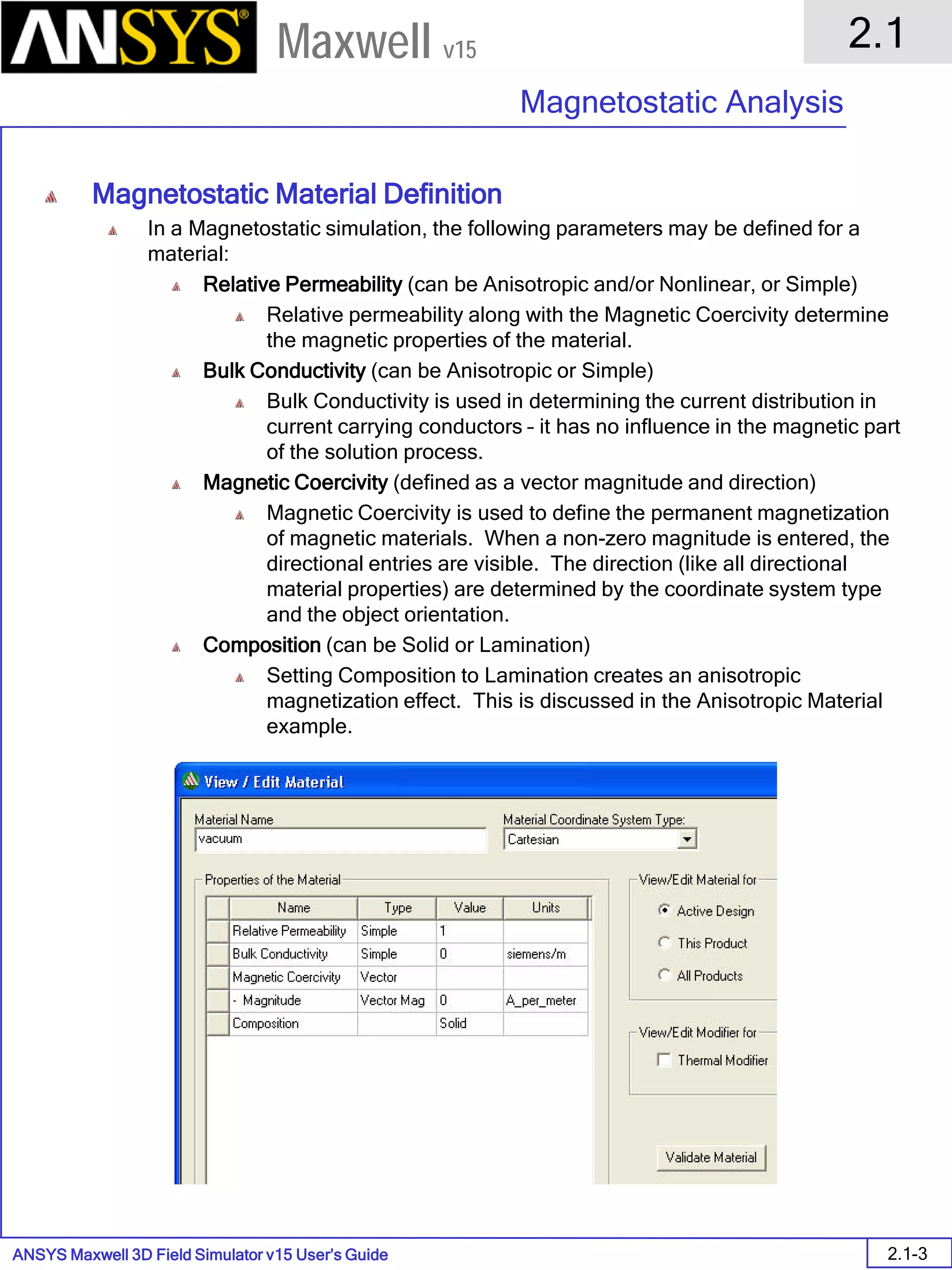
Solution Types and Solvers
2.0-4
Maxwell v15
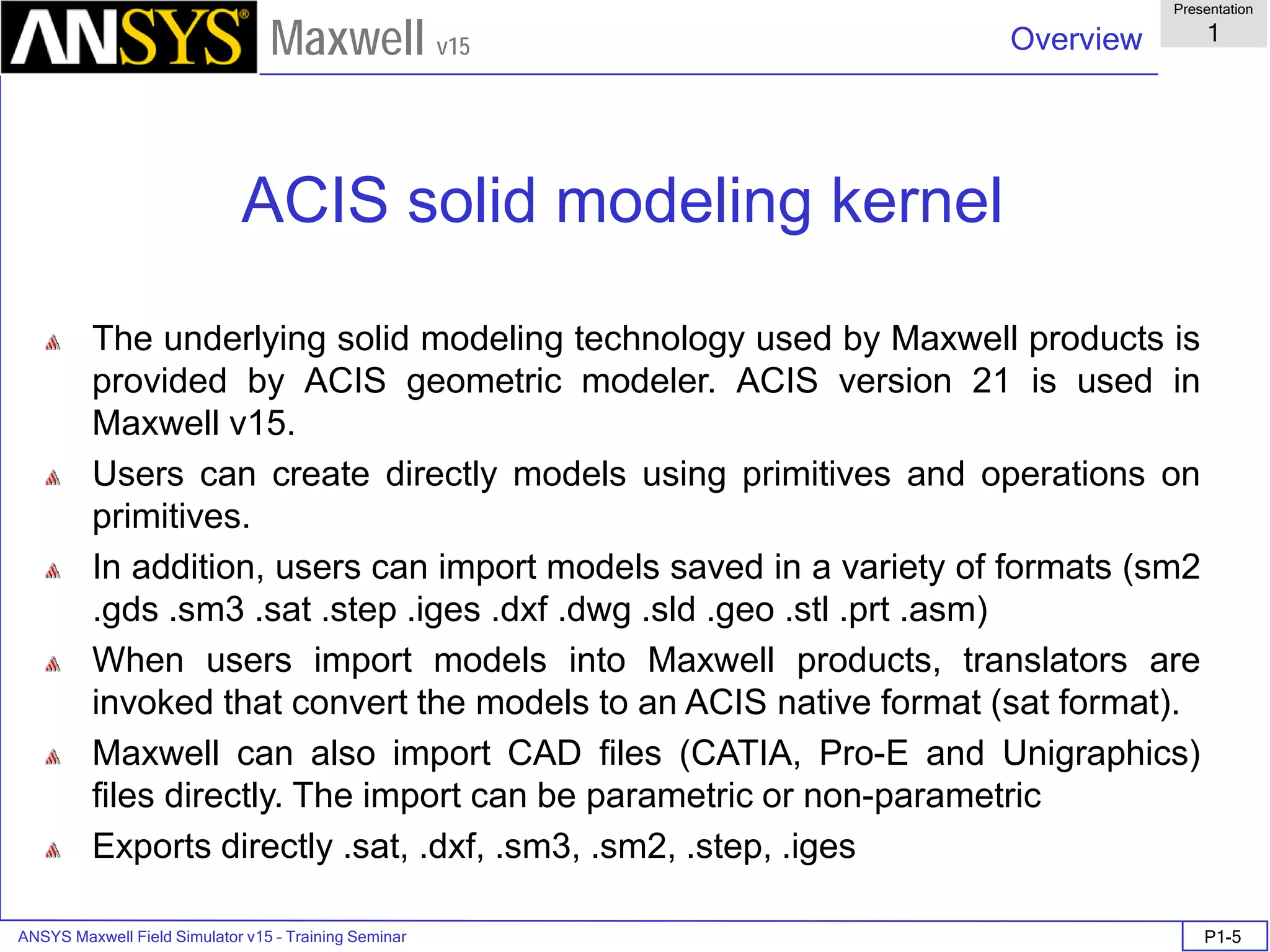
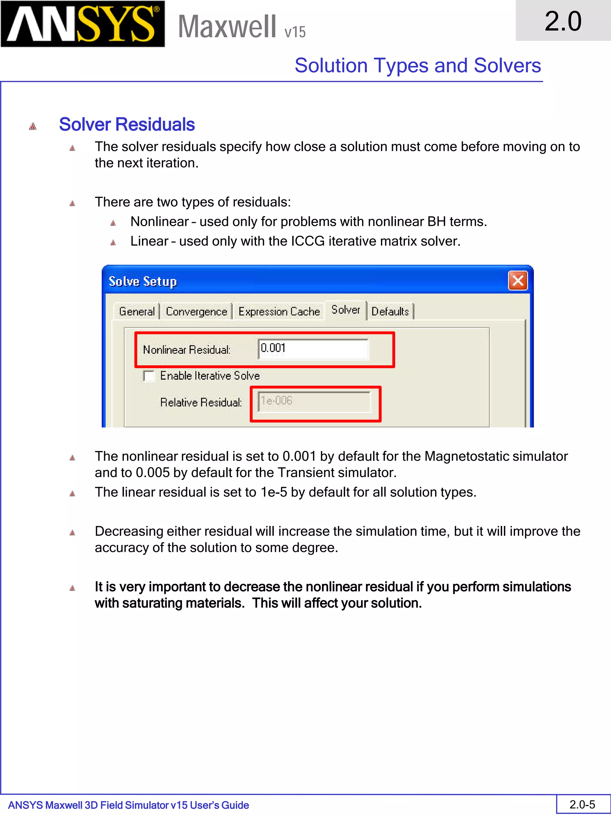
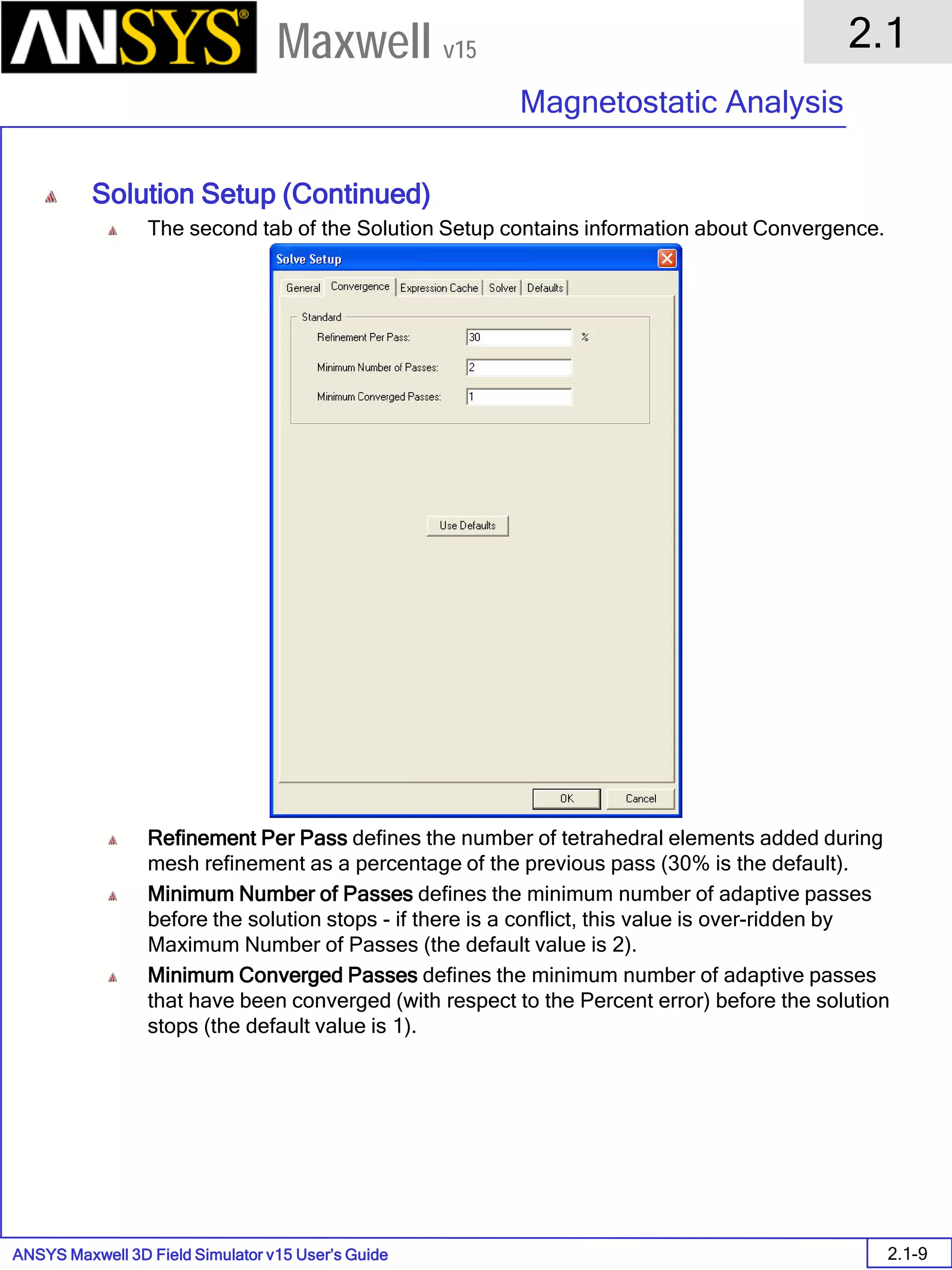
General Finite Element Method Information (Continued)
Once the tetrahedra are defined, the finite elements are placed in a large, sparse
matrix equation.
This can now be solved using standard matrix solution techniques such as:
Sparse Gaussian Elimination (direct solver)
Incomplete Choleski Conjugate Gradient Method (ICCG iterative solver)
It should be noted that the direct solver is the default solver, and is generally the
best method. The ICCG solver is included for special cases and for reference.
Error Evaluation
For each solver, there is some fundamental defining equation that provides an
error evaluation for the solved fields. In the case of the magnetostatic simulation,
this defining equation is the no-monopoles equation, which says:
When the field solution is returned to this equation, we get an error term:
The energy produced by these error terms (these errors act in a sense like
sources) is computed in the entire solution volume. This is then compared with
the total energy calculated to produce the percent error energy number.
This number is returned for each adaptive pass along with the total energy, and
these two numbers provide some measure of the convergence of the solution.
Remember that this is a global measure of the convergence – local errors can
exceed this percentage.
[ ][ ] [ ]JHS =
0=⋅∇ B
errBsolution =⋅∇
%100×=
energytotal
energyerror
energyerrorpercent](https://image.slidesharecdn.com/maxwell3d-160822035138/75/Maxwell3-d-118-2048.jpg)


![ANSYS Maxwell Field Simulator v15 – Training Seminar 3.3-9
Overview
Presentation
3.3
Maxwell v15
Adaptive Mesh Refinement
Mesh after 2 passes
Convergence
EnergyError[%]
Pass](https://image.slidesharecdn.com/maxwell3d-160822035138/75/Maxwell3-d-271-2048.jpg)
![ANSYS Maxwell Field Simulator v15 – Training Seminar 3.3-10
Overview
Presentation
3.3
Maxwell v15
Adaptive Mesh Refinement
Mesh after 4 passes
Convergence
EnergyError[%]
Pass](https://image.slidesharecdn.com/maxwell3d-160822035138/75/Maxwell3-d-272-2048.jpg)
![ANSYS Maxwell Field Simulator v15 – Training Seminar 3.3-11
Overview
Presentation
3.3
Maxwell v15
Adaptive Mesh Refinement
Mesh after 6 passes
Convergence
EnergyError[%]
Pass](https://image.slidesharecdn.com/maxwell3d-160822035138/75/Maxwell3-d-273-2048.jpg)
![ANSYS Maxwell Field Simulator v15 – Training Seminar 3.3-12
Overview
Presentation
3.3
Maxwell v15
Adaptive Mesh Refinement
Mesh after 10 passes
Convergence
EnergyError[%]
Pass](https://image.slidesharecdn.com/maxwell3d-160822035138/75/Maxwell3-d-274-2048.jpg)
![ANSYS Maxwell Field Simulator v15 – Training Seminar 3.3-13
Overview
Presentation
3.3
Maxwell v15
Adaptive Mesh Refinement
Mesh after 16 passes.
Desired Energy Error of 0.2% is reached
Convergence
EnergyError[%]
Pass](https://image.slidesharecdn.com/maxwell3d-160822035138/75/Maxwell3-d-275-2048.jpg)

![ANSYS Maxwell Field Simulator v15 – Training Seminar 3.3-15
Overview
Presentation
3.3
Maxwell v15
Adaptive Mesh Refinement
Energy Error goal reduced further.
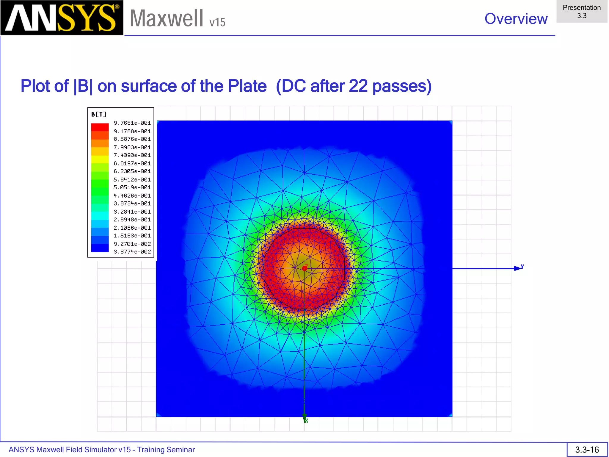
Mesh after 22 passes. Desired
Energy Error of 0.03% is reached
Convergence
EnergyError[%]
Pass](https://image.slidesharecdn.com/maxwell3d-160822035138/75/Maxwell3-d-277-2048.jpg)
![ANSYS Maxwell Field Simulator v15 – Training Seminar 3.3-17
Overview
Presentation
3.3
Maxwell v15
Convergence
Even in the region of the convergence
curve above pass number 16, a
gradient in the energy error from pass
to pass can be observed.
Continued iteration results in higher
accuracy but at a cost of a large
number of tetrahedrons.
Clearly a tradeoff must be found
EnergyError[%]
EnergyError[%]
Pass
Pass
No.TetsDeltaEnergy[%]](https://image.slidesharecdn.com/maxwell3d-160822035138/75/Maxwell3-d-279-2048.jpg)
![ANSYS Maxwell Field Simulator v15 – Training Seminar 3.3-18
Overview
Presentation
3.3
Maxwell v15
Convergence definition through use of additional variables
% Change in the Force on the magnet can be used to determine a more effective
stopping criteria since this value can be tied directly to the acceptable numerical
tolerance on a physical variable
DeltaForce[%]
DeltaForce[%]
Pass
Pass](https://image.slidesharecdn.com/maxwell3d-160822035138/75/Maxwell3-d-280-2048.jpg)


![ANSYS Maxwell 3D Field Simulator v15 User’s Guide
5.5
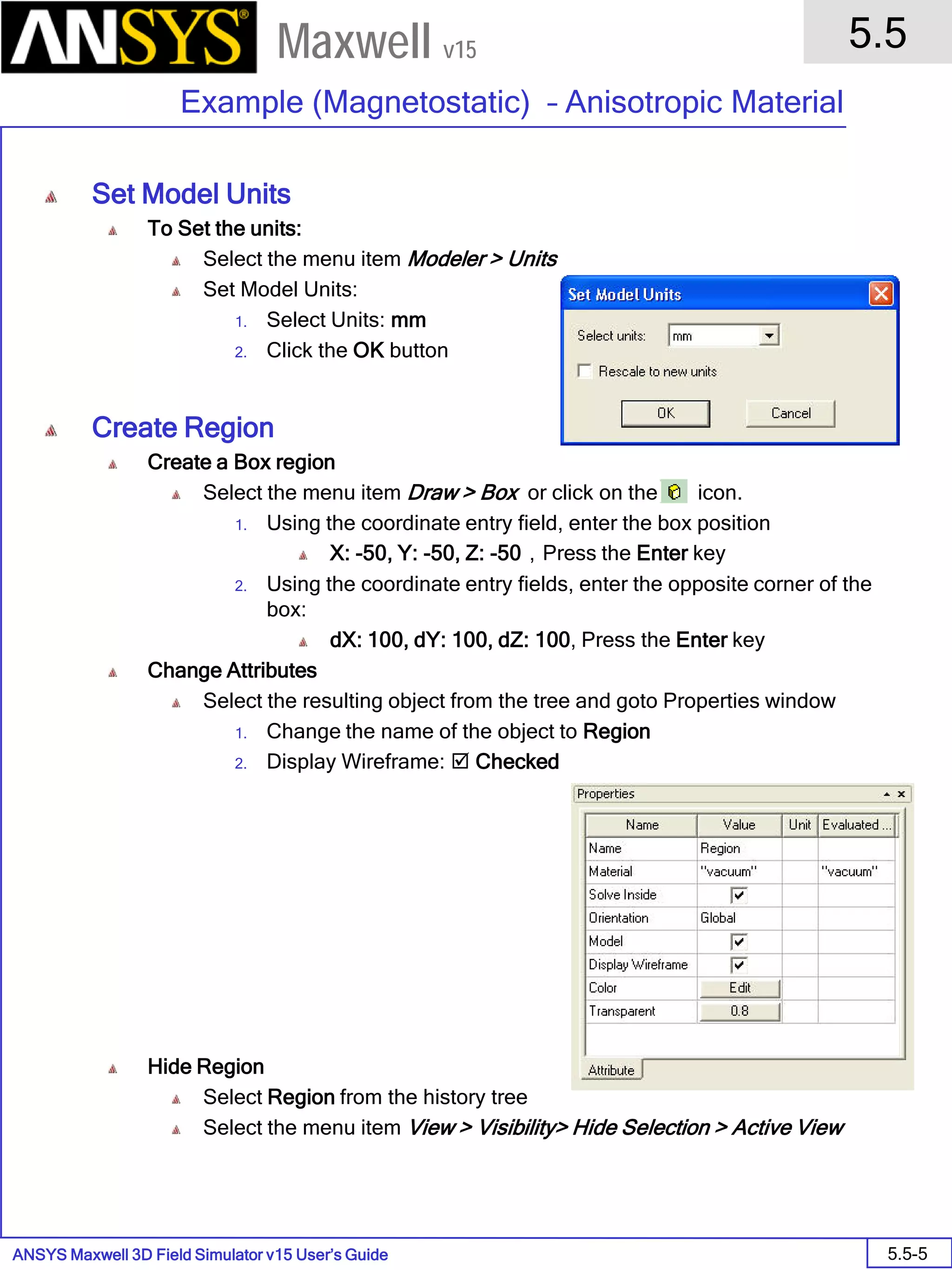
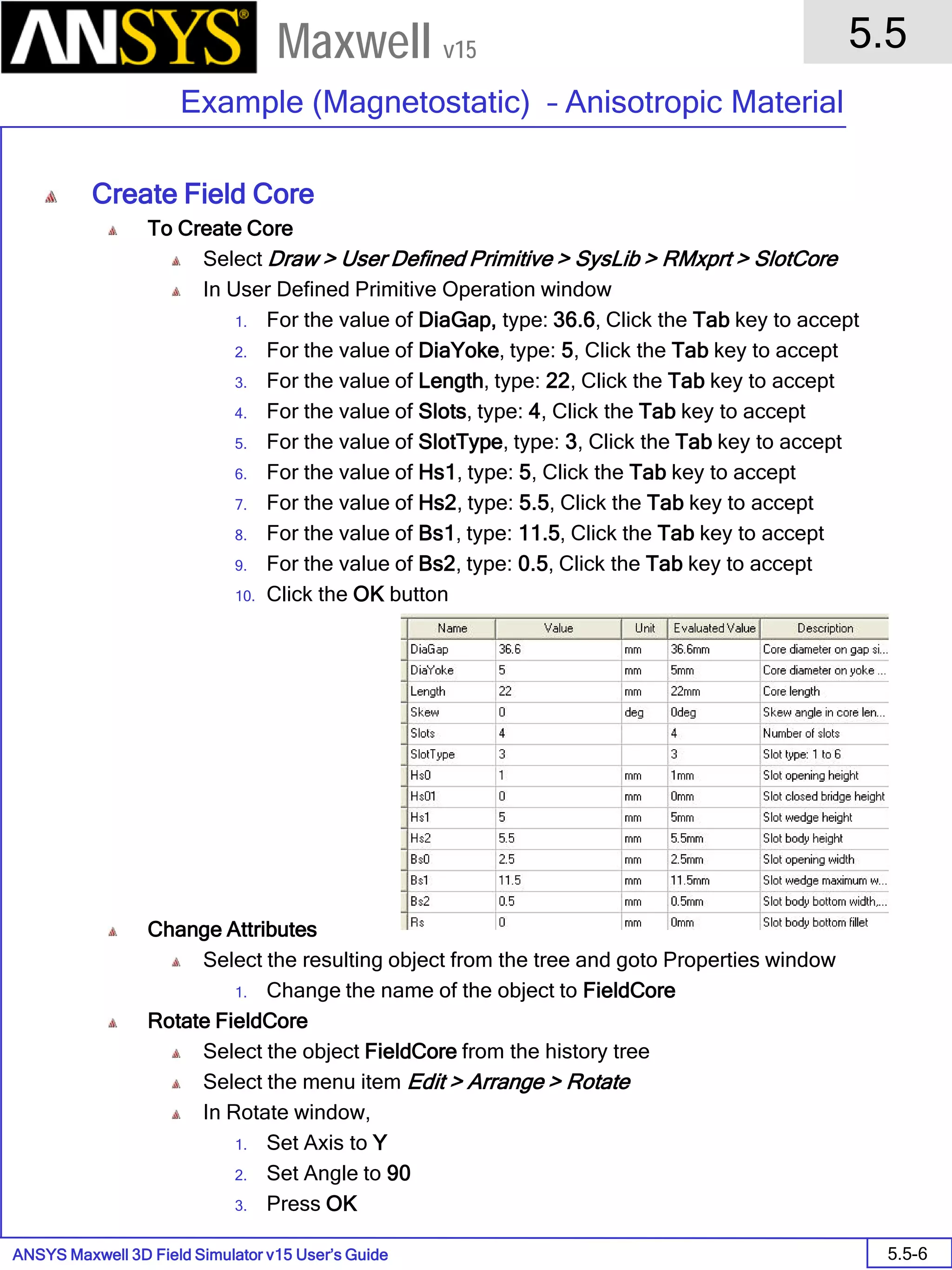
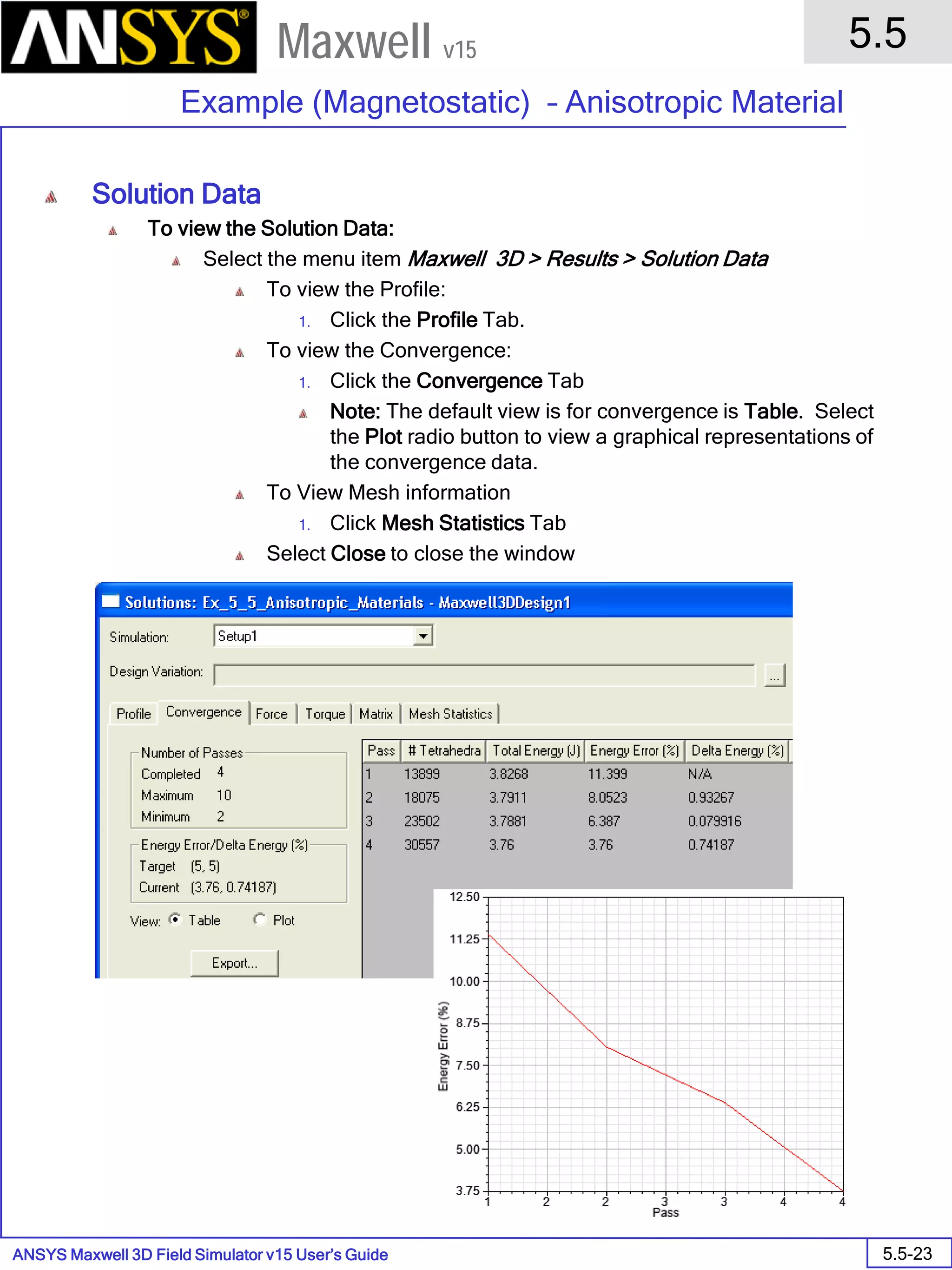
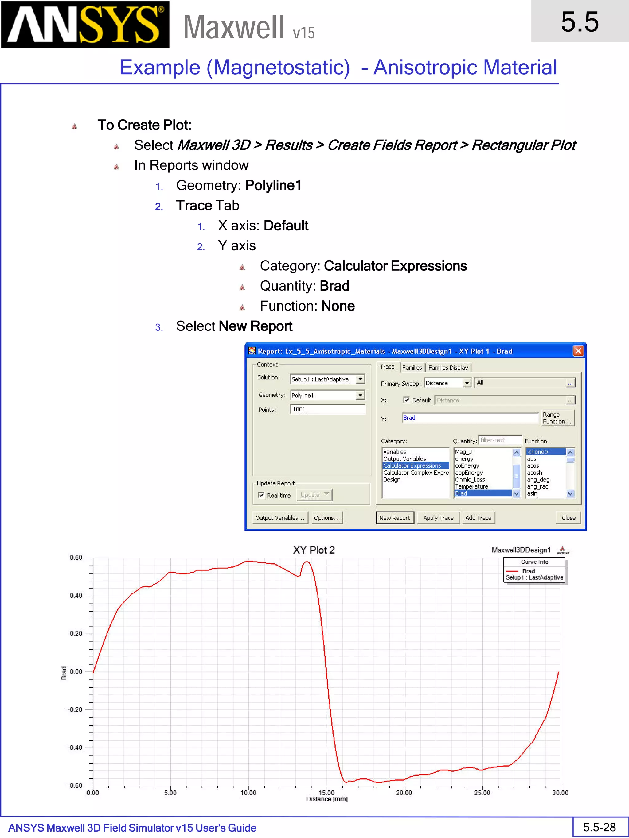
Example (Magnetostatic) – Anisotropic Material
5.5-7
Maxwell v15
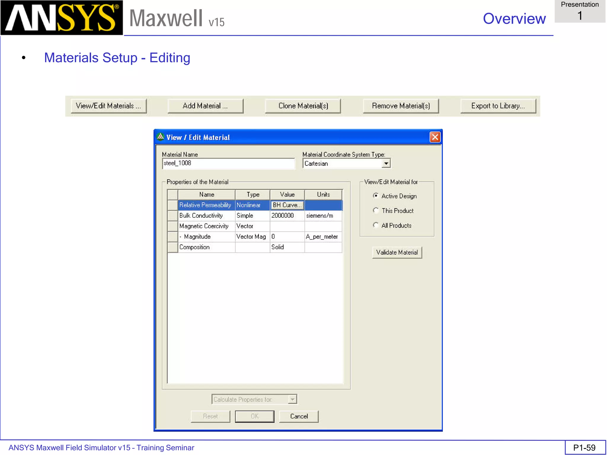
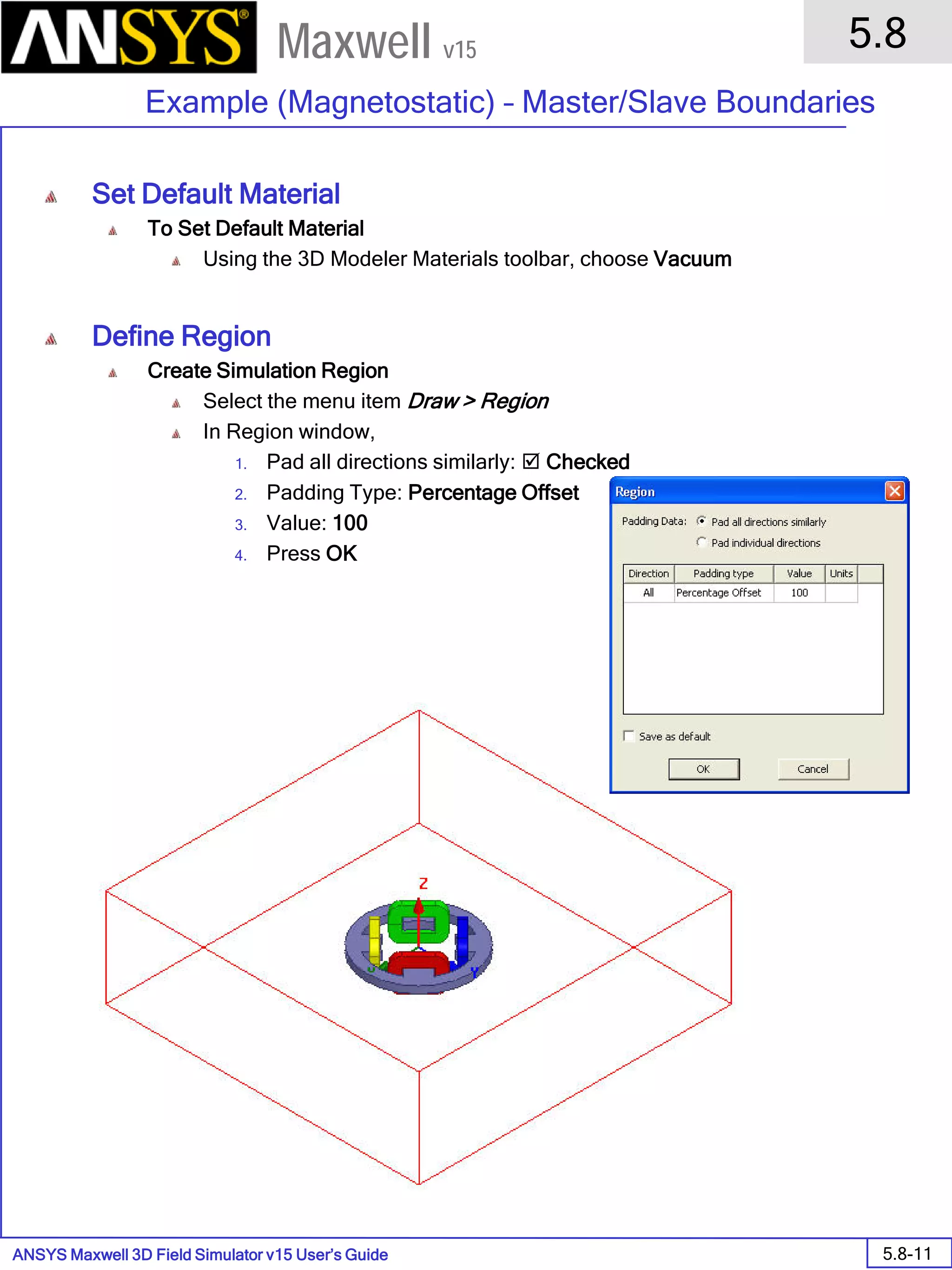
Define Material for FieldCore
To Create Material
Select the object FieldCore from the history tree, right click and select
Assign Material
In Select Definition window,
1. Select option Add Material
2. In View/Edit Material window
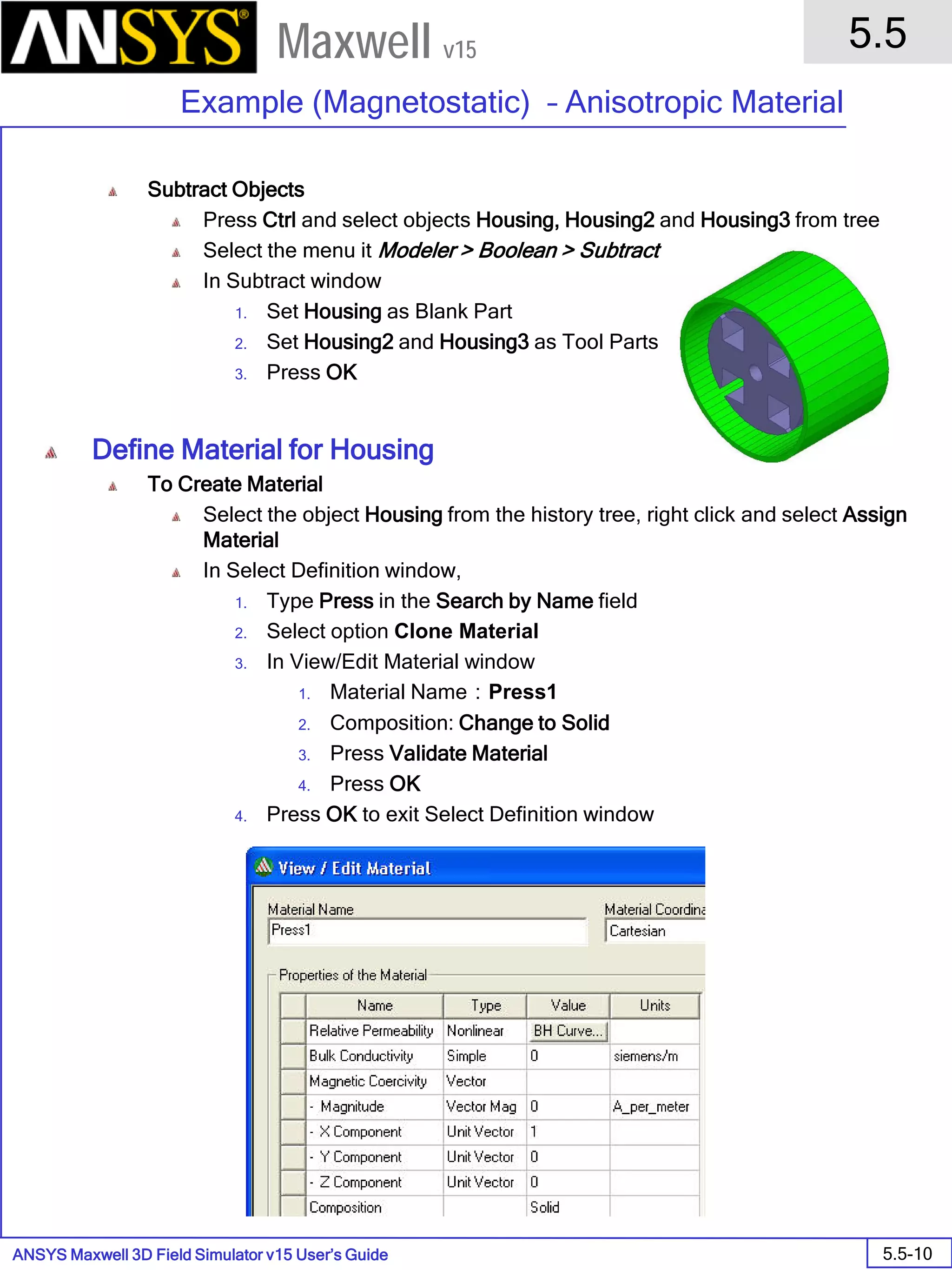
1. Material Name:Press
2. Relative Permeability
Change Type to Nonlinear
Click the BH Curve tab that will appear in Value field
In BH Curve window,
1. Select Import Dataset
2. Change File type to Tab Delimited data file
3. Locate the file Press.tab and Open it
4. Press OK to close BH Curve window
3. Composition: Change to Lamination
Stacking Factor: 0.95
Stacking Direction: V(1) [X Direction]
4. Press Validate Material
5. Press OK
3. Press OK to exit Select Definition window](https://image.slidesharecdn.com/maxwell3d-160822035138/75/Maxwell3-d-427-2048.jpg)


![ANSYS Maxwell 3D Field Simulator v15 User’s Guide
5.5
Example (Magnetostatic) – Anisotropic Material
5.5-22
Maxwell v15
1
The Modeling Sequence will be as follows:
Reference:
[1] D. Lin, P. Zhou, Z. Badics, W. N. Fu, Q. M. Chen and Z. J. Cendes, “A New Nonlinear
Anisotropic Model for Soft Magnetic Materials” , CSY0084 of COMPUMAG’2005](https://image.slidesharecdn.com/maxwell3d-160822035138/75/Maxwell3-d-442-2048.jpg)


![ANSYS Maxwell 3D Field Simulator v15 User’s Guide
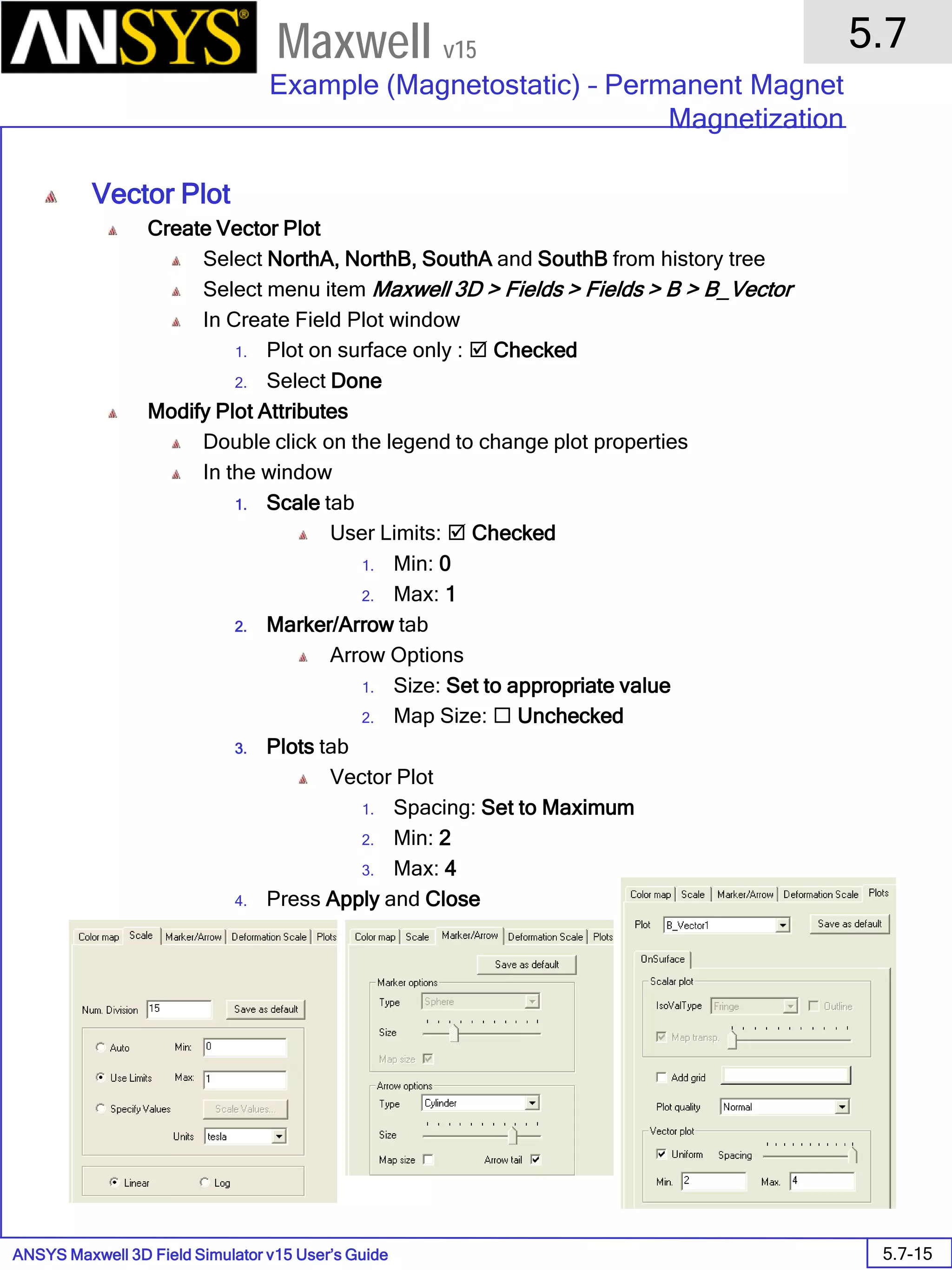
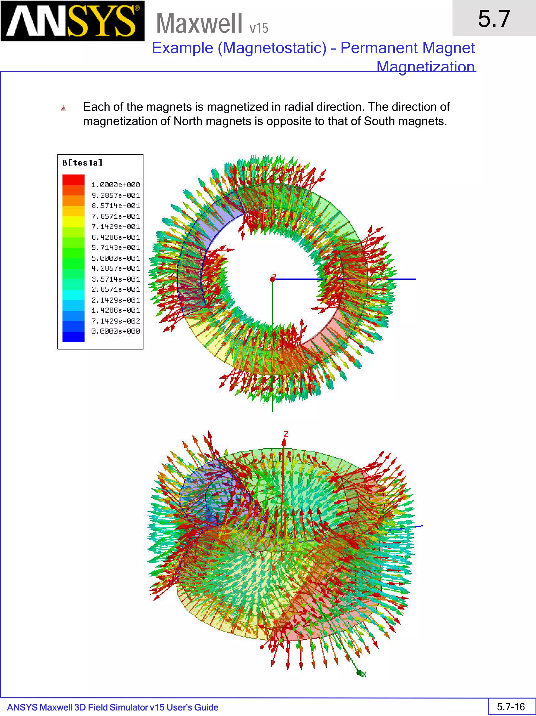
5.7
Example (Magnetostatic) – Permanent Magnet
Magnetization
5.7-21
Maxwell v15
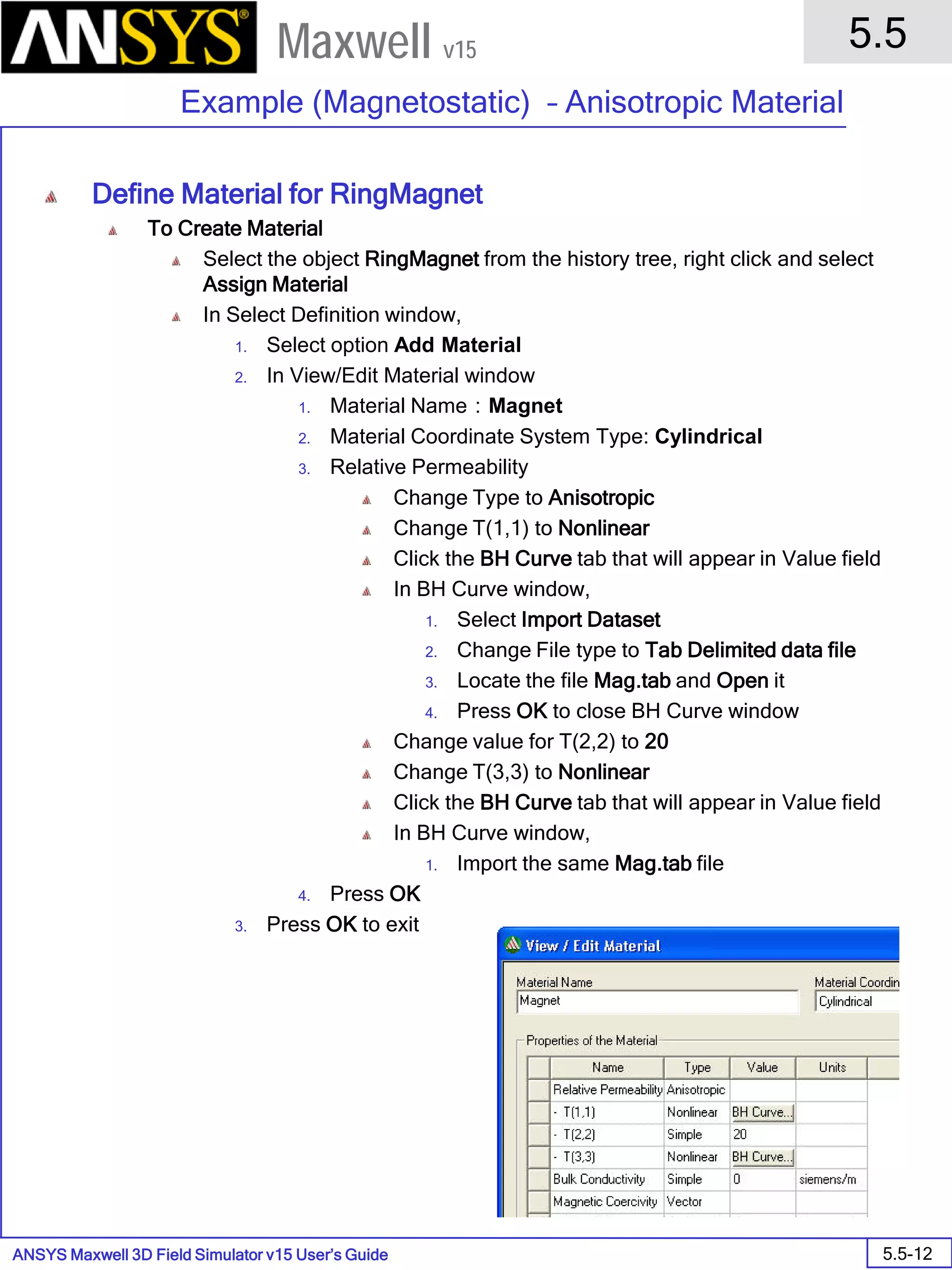
Create New Material: Magnet_Equation
To Create material Magnet_Equation:
Select RingMagnet from the history tree, right click and select Assign
Material
In Select Definition window,
1. Select option Clone Material
2. In View/Edit Material window
1. Material Name:Magnet_Equation
2. Magnitude:-890000
3. R Component: sin (2*(Phi - 0.785*(Z/40mm)))
4. Press OK
3. select OK.
Note:About the equation
The equations used in this case is a sine function which switches the value
of R from positive to negative with Phi hence altering the direction of
magnetization. Rest of the equation gives skew to the direction along Z
direction. This gives the field similar to four pole magnet with 45 degree
skew modeled in last exercise
sin (2*(Phi - 0.785*(Z/40mm)))
Number of Poles / 2
Skew angle in radians[45 deg] Length of magnet](https://image.slidesharecdn.com/maxwell3d-160822035138/75/Maxwell3-d-493-2048.jpg)


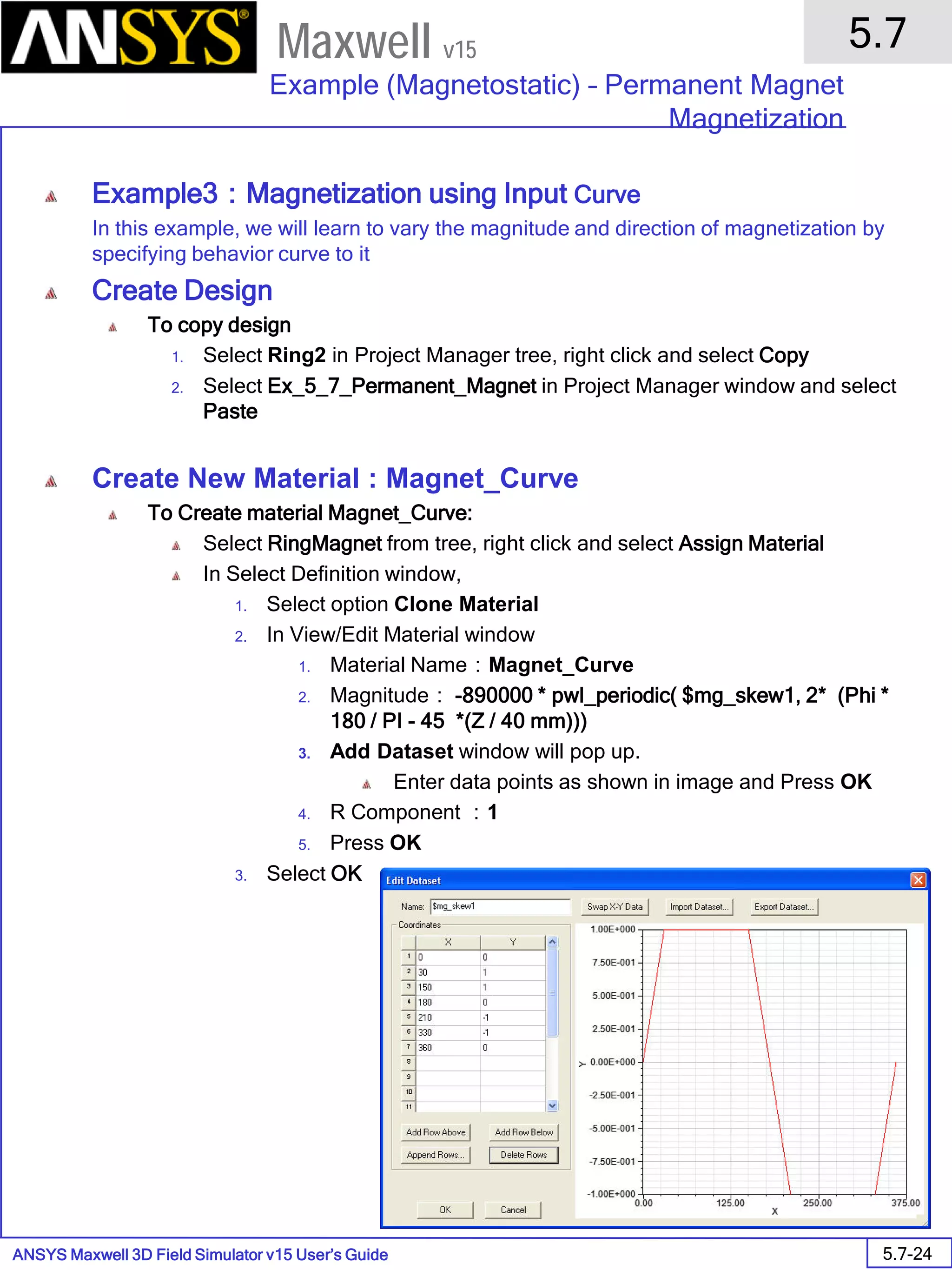
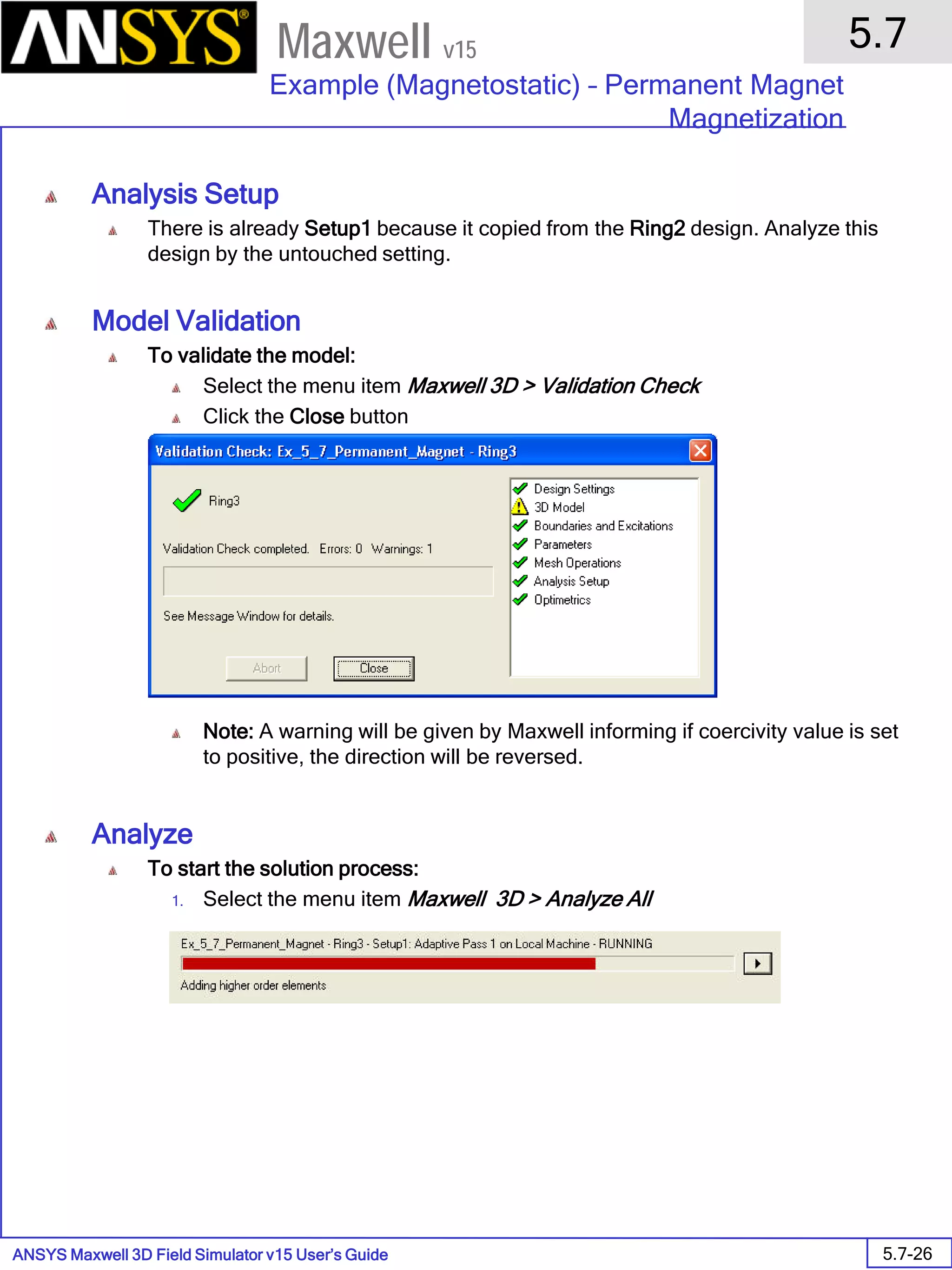
![ANSYS Maxwell 3D Field Simulator v15 User’s Guide
5.7
Example (Magnetostatic) – Permanent Magnet
Magnetization
5.7-25
Maxwell v15
Note:About the function
The function which has been specified in the material definition sets a multiplier
$mg_skew1 for the magnitude of magnetic coercivity.
Input curve that we specified varies the multiplier $mg_Skew1 from +1 to -1 with
the change in value of Phi. Hence it varies the direction of magnetization of
magnets.
Number of poles value will multiply the value of Phi. Hence ensuring value of
$mag_skew1 cycles twice in single rotation of Phi. This results two peaks (North
Pole) and two valleys (South Pole) giving a four pole magnet.
Moreover, to apply the skew, magnetic data is rotated with Z axis coordinates.
$CoreOrigin defines the Z position where value of $mg_skew becomes zero. In
our case this value is 0mm. Hence it is not considered in the function specified.
X : Phi = 0
Skew angle
$Height
$CoreOrigin
-837999 * pwl_periodic( $mg_skew1, 2* (Phi*180/PI - 45 *((Z- $CoreOrigin / 2 mm)))
Magnetization Number of Poles
Skew angle[deg]
0 position
Length of magnetMagnetization wave form](https://image.slidesharecdn.com/maxwell3d-160822035138/75/Maxwell3-d-497-2048.jpg)


![ANSYS Maxwell 3D Field Simulator v15 User’s Guide
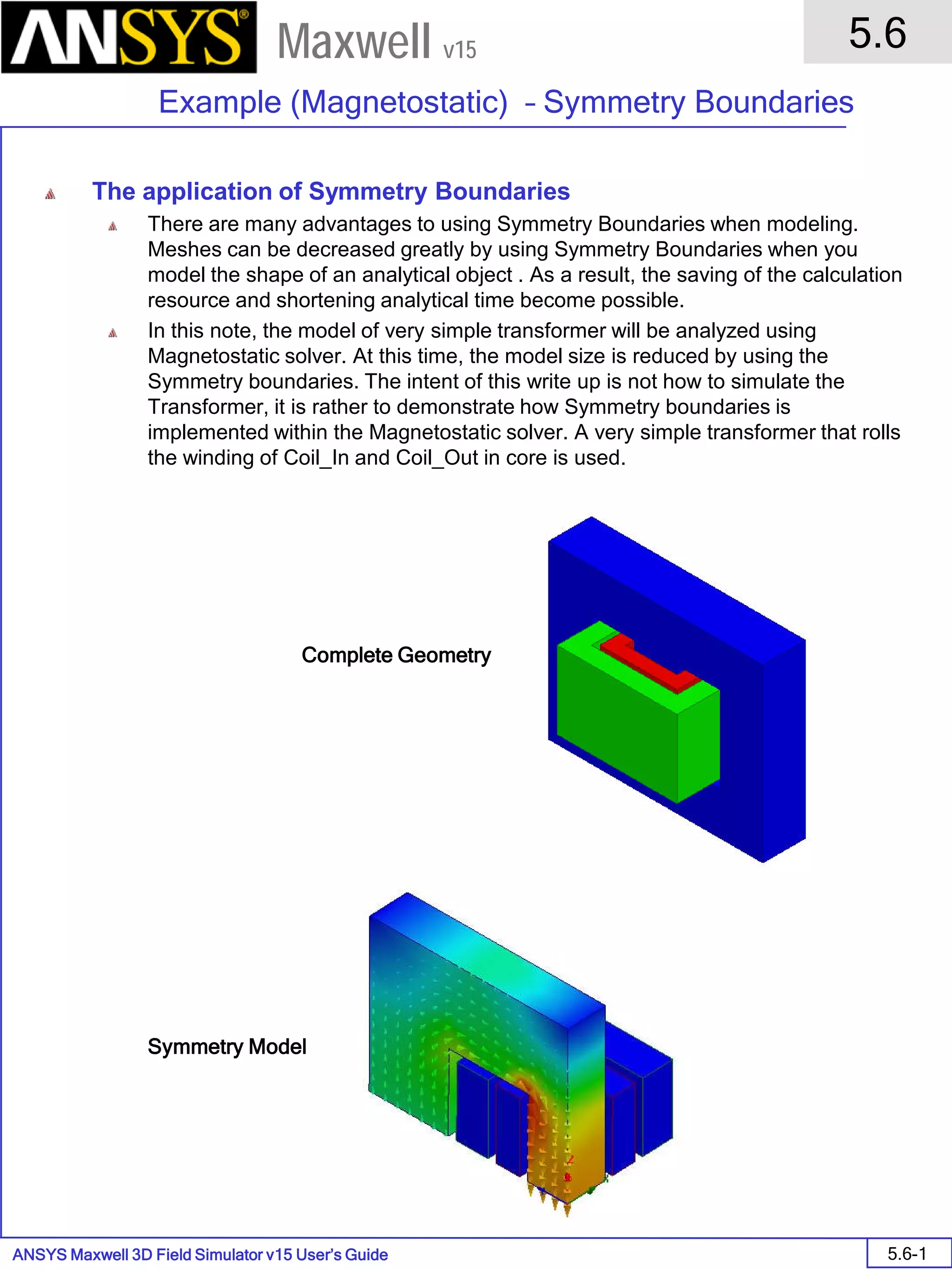
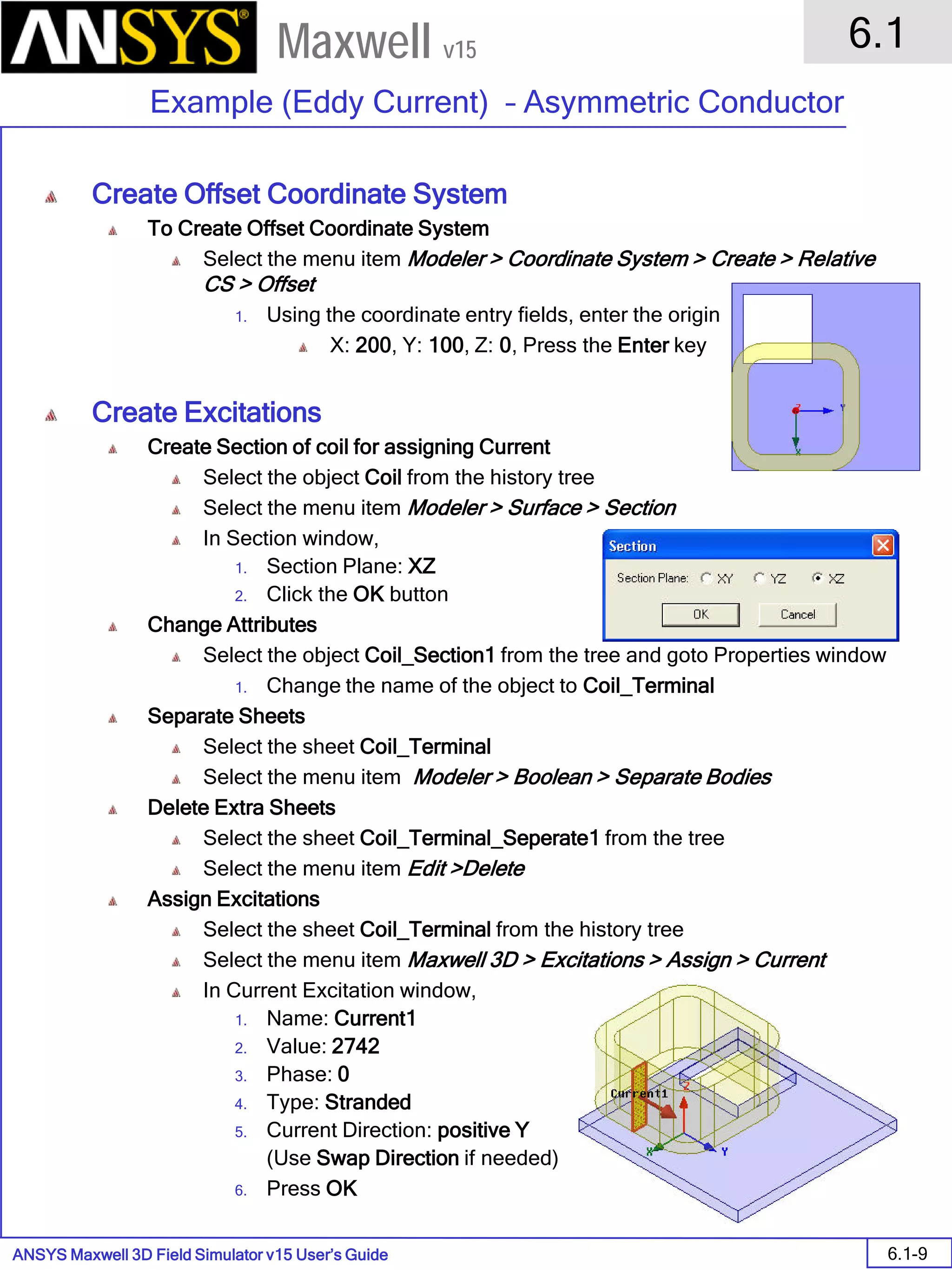
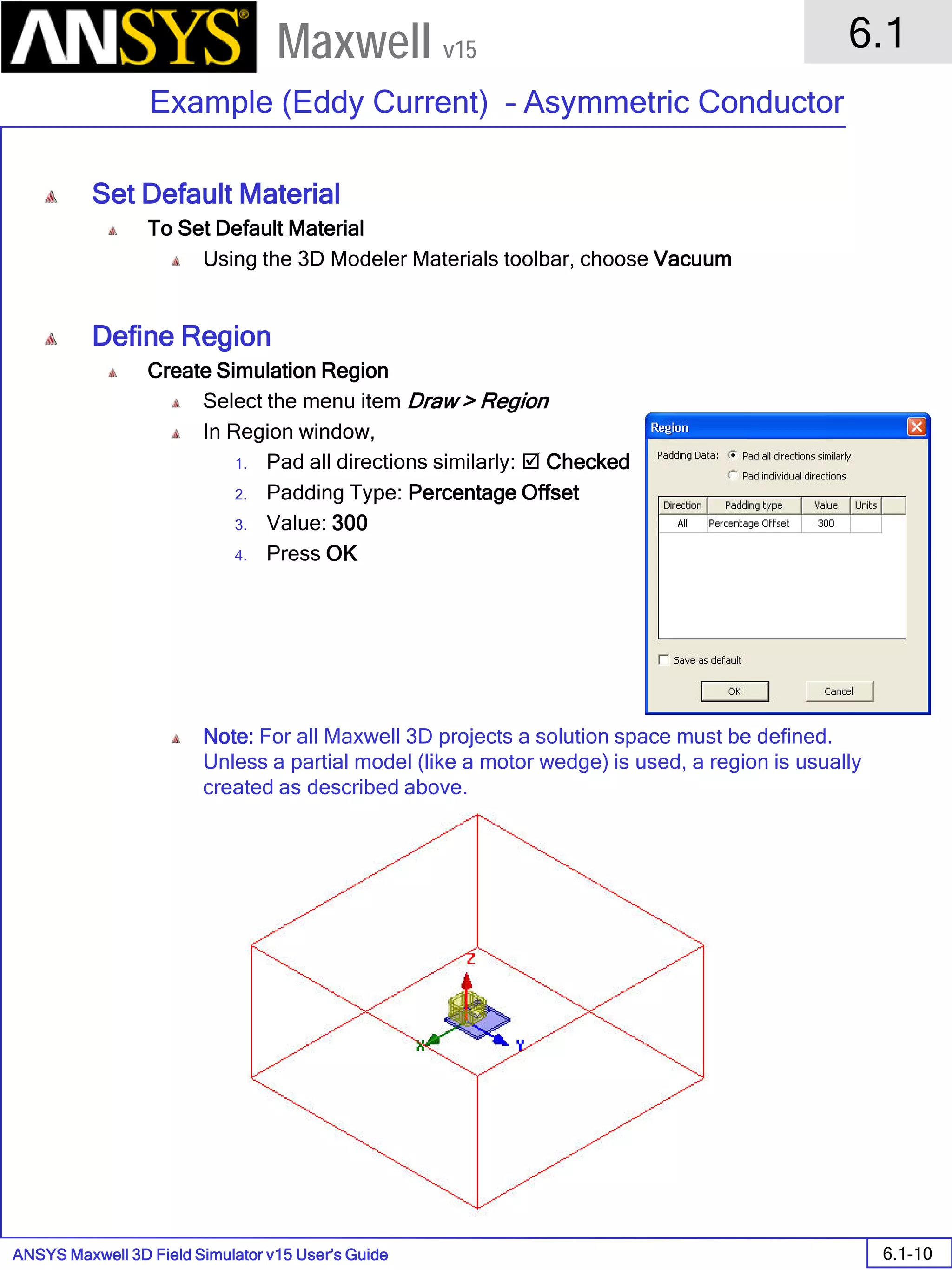
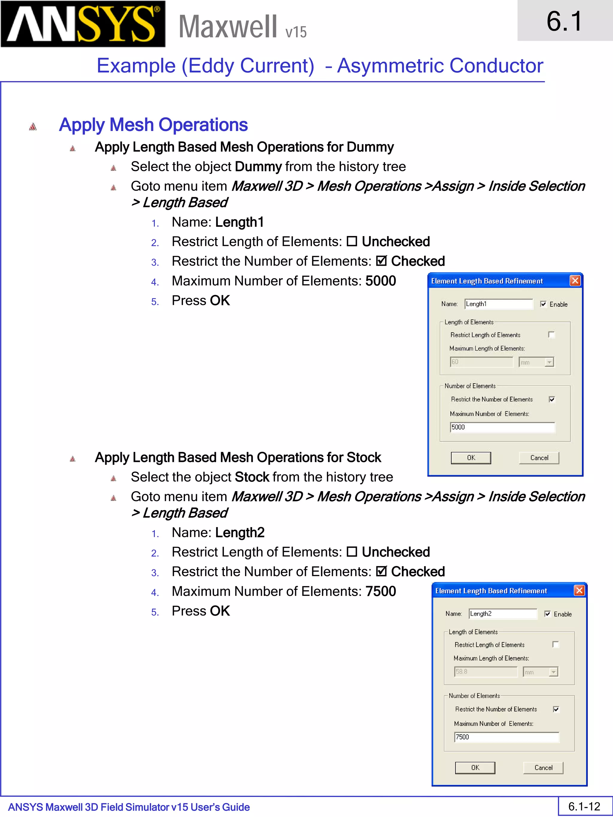
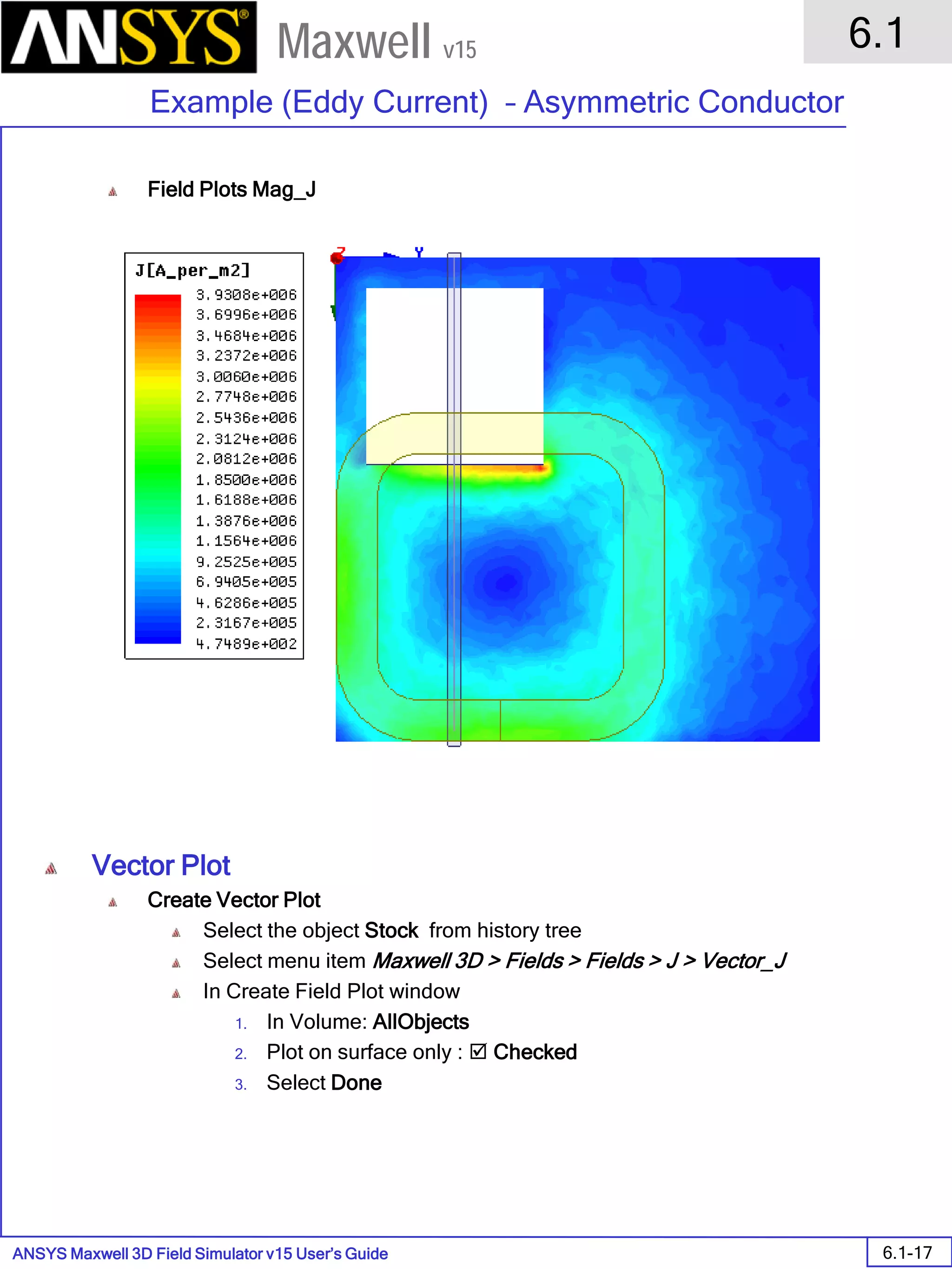
6.1
Example (Eddy Current) – Asymmetric Conductor
6.1-11
Maxwell v15
Create Dummy Object
Note: As a post-processing results we are interested to calculate the flux density
on a line with the following end points: [0; 72; 34] and [288; 72; 34]. In order to
get as accurate results as possible, the mesh around the line has to be fine
enough. It is generally a good practice to create dummy objects around regions
of interest so that the mesh quality can be better controlled in those regions. For
this particular problem we create a box around the line of interest.
Change Work Coordinate System
Goto Modeler > Coordinate System > Set Working CS
In Select Coordinate System Window
1. Select Global
2. Press Select
To Create Dummy Object
Select the menu item Draw > Box
1. Using the coordinate entry fields, enter the box position
X: -3, Y: 68, Z: 30, Press the Enter key
2. Using the coordinate entry fields, enter the opposite corner of the
box: (in Absolute values)
X: 297, Y: 76, Z: 38, Press the Enter key
Change Attributes
Select the resulting object from the tree and goto Properties window
1. Change the name of the object to Dummy
Set Eddy Effects
To Set Eddy Effects
Select the menu item Maxwell 3D > Excitations > Set Eddy Effect
In Set Eddy Effects window
1. Eddy Effects:
Stock: Checked
Coil: UnChecked
2. Displacement Current:
Coil and Stock : Unchecked
3. Press OK](https://image.slidesharecdn.com/maxwell3d-160822035138/75/Maxwell3-d-539-2048.jpg)

![ANSYS Maxwell 3D Field Simulator v15 User’s Guide
6.1
Example (Eddy Current) – Asymmetric Conductor
6.1-14
Maxwell v15
Create Objects for Rectangular Plot
To Create Line Object
Select menu item Draw > Line
A massage will pop up asking if the entity needs to be created as non
model object. Select Yes to it.
1. Using Co-ordinate entry field Enter the first vertex
X = 0, Y = 72, Z = 34, Press Enter
2. Using Co-ordinate entry field Enter the second vertex
X = 288, Y = 72, Z = 34, Press Enter
Change Attributes
Select the resulting object from the tree and goto Properties window
1. Change the name of the object to FieldLine
Create Parameters
Create parameter Bz_real
Go to Maxwell 3D > Fields > Calculator
1. Select Input > Quantity > B
2. Select Vector > Scal? > ScalarZ
3. Select General > Complex > Real
4. Select General > Smooth
Note: The flux density will be displayed by default in the units of
Tesla [T]. If you wish to see the results in Gaussian units perform
steps 5 and 6, otherwise jump to step 7
5. Select Input > Number
Type: Scalar
Value: 10000
Press OK
6. Select General > *
7. Select Add and set the name of expression as Bz_real](https://image.slidesharecdn.com/maxwell3d-160822035138/75/Maxwell3-d-542-2048.jpg)
![ANSYS Maxwell 3D Field Simulator v15 User’s Guide
6.1
Example (Eddy Current) – Asymmetric Conductor
6.1-15
Maxwell v15
Create parameter Bz_imag
Go to Maxwell 3D > Fields > Calculator
1. Select Input > Quantity > B
2. Select Vector > Scal? > ScalarZ
3. Select General > Complex > Imag
4. Select General > Smooth
Note: The flux density will be displayed by default in the units of
Tesla [T]. If you wish to see the results in Gaussian units perform
steps 5 and 6, otherwise jump to step 7
5. Select Input > Number
Type: Scalar
Value: 10000
Press OK
6. Select General > *
7. Select Add and set the name of expression as Bz_imag
8. Press Done
Rectangular Plot
To Create Plot:
Select Maxwell 3D > Results > Create Fields Report > Rectangular Plot
In Reports window
1. Geometry: FieldLine
2. Trace Tab
1. X axis: Default
2. Y axis
Category: Calculator Expressions
Quantity: Bz_real
Function: None
3. Select New Report
4. Without closing window, change quantity to Bz_imag
5. Select Add Trace
6. Select Close](https://image.slidesharecdn.com/maxwell3d-160822035138/75/Maxwell3-d-543-2048.jpg)


![ANSYS Maxwell 3D Field Simulator v15 User’s Guide
9.15
Basic Exercises – PM Assignment
9.15-5
Maxwell v15
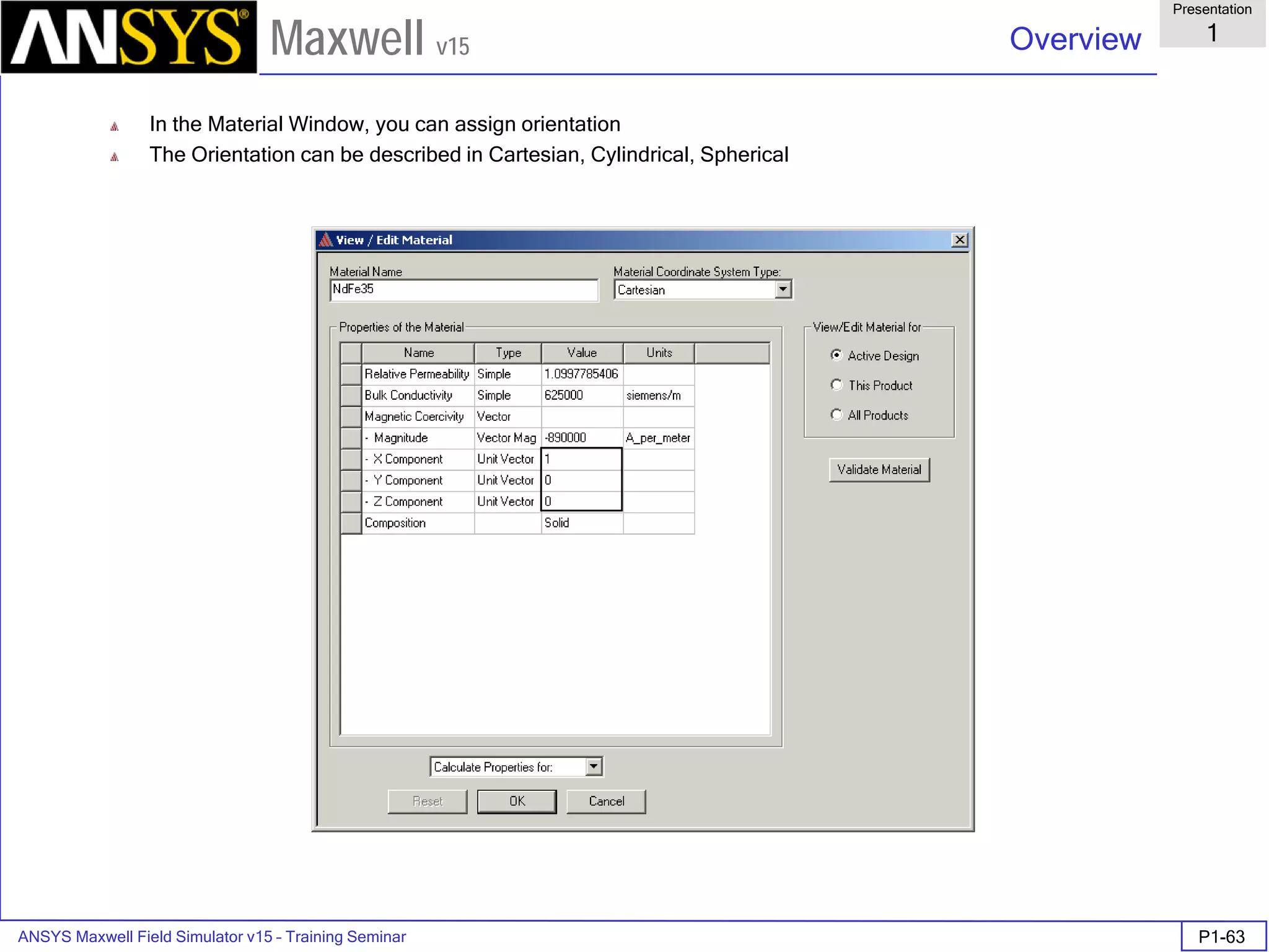
The direction of magnetization is specified by a unit vector relative to the
Coordinate System (CS) associated with the given object, that is relative to
the Orientation of the object. If the Orientation of the object is Global, the
unit vector will be specified relative to the Global CS. Maxwell also allows
to specify the type of the Coordinate System (upper right corner ). Thus
Cartesian, Cylindrical and Spherical CS type can be defined. This means
that if the Orientation of the object is Global and CS type Cartesian, the unit
vector will be specified as X, Y, and Z relative to the Cartesian Global CS.
Hence, the right direction of magnetization is specified by the appropriate
combination of object’s Orientation, CS type and Unit Vector.
For this particular magnet definition, the unit vector is [1,0,0]. This means
that if the magnet remains oriented in the Global CS, the magnet will be
magnetized in the Global X direction.
In order to change this direction, we either change the unit vector or define
a new coordinate system and associate the magnet with it. The X-axis of
the new CS will have point in the direction of magnetization as the original
(default) unit vector [1,0,0] in this case remains unchanged.
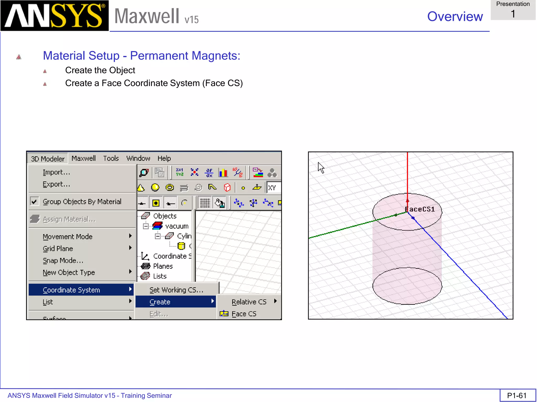
The most advantageous is creation of FACE coordinate systems, which is
discussed in the following.](https://image.slidesharecdn.com/maxwell3d-160822035138/75/Maxwell3-d-831-2048.jpg)