Downloaded 18 times


![Conclusions
For quadratic problems, all methods gives satisfactory results.
Powell’s method is working satisfactorily for small (i.e.lower-dimensional)
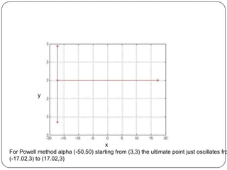
problems [particularly for α=(-5,20)]
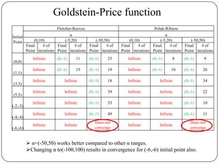
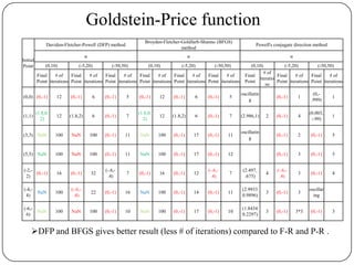
DFP-BFGS works very good for bad functions (e.g Goldstein Price
function) where F-R and P-R does not work well.
Suitability of DFP, BFGS for higher dimensional problems need to be
studied more.
Range of step size if chosen small and searches on both side of the given
point [α=(-5,20)], it works well for all problems.](https://image.slidesharecdn.com/comparativestudyofalgorithmsofnonlinearoptimizationfinal-130511131735-phpapp02/85/Comparative-study-of-algorithms-of-nonlinear-optimization-44-320.jpg)


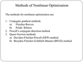
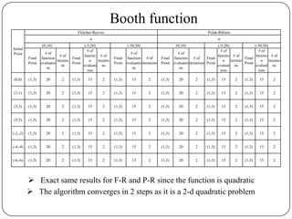
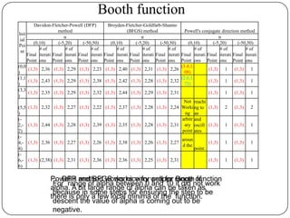
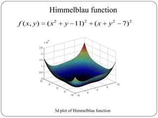
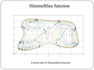
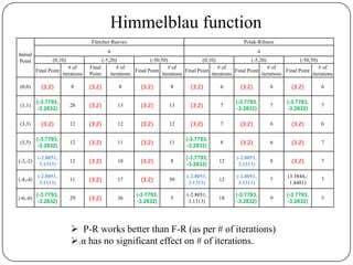
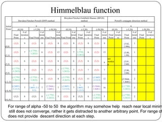
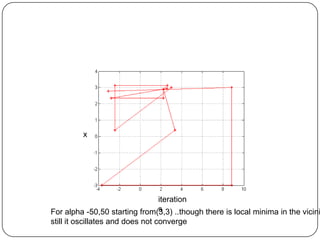
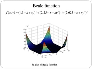
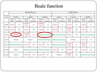
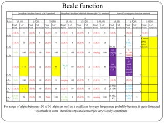
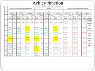
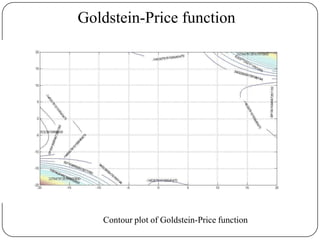
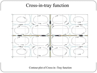
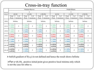
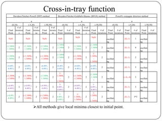
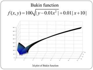
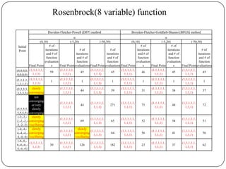
The document presents a comparative study of algorithms for nonlinear optimization. It evaluates several nonlinear optimization algorithms (conjugate gradient methods, quasi-Newton methods, Powell's method) on standard test functions (Booth, Himmelblau, Beale) from different initial points and step sizes. For the Booth function, all algorithms converge in 2 steps. For Himmelblau, Polak-Ribiere and BFGS methods perform best. For Beale, conjugate gradient methods converge for some initial points but not all, while Powell's method converges from more points.