Download as PDF, PPTX


![Simulated Annealing: Part 2
Cooling Schedule
Geometric
– In the geometric schedule, the temperature is updated
using the formula
Ti+1 = α.Ti
– where α ∈]0, 1[.– where α ∈]0, 1[.
– It is the most popular cooling function.
– Experience has shown that α should be between 0.5 and
0.99.](https://image.slidesharecdn.com/simulatedannealing-150110102506-conversion-gate01/75/Simulated-annealing-ppt-22-2048.jpg)


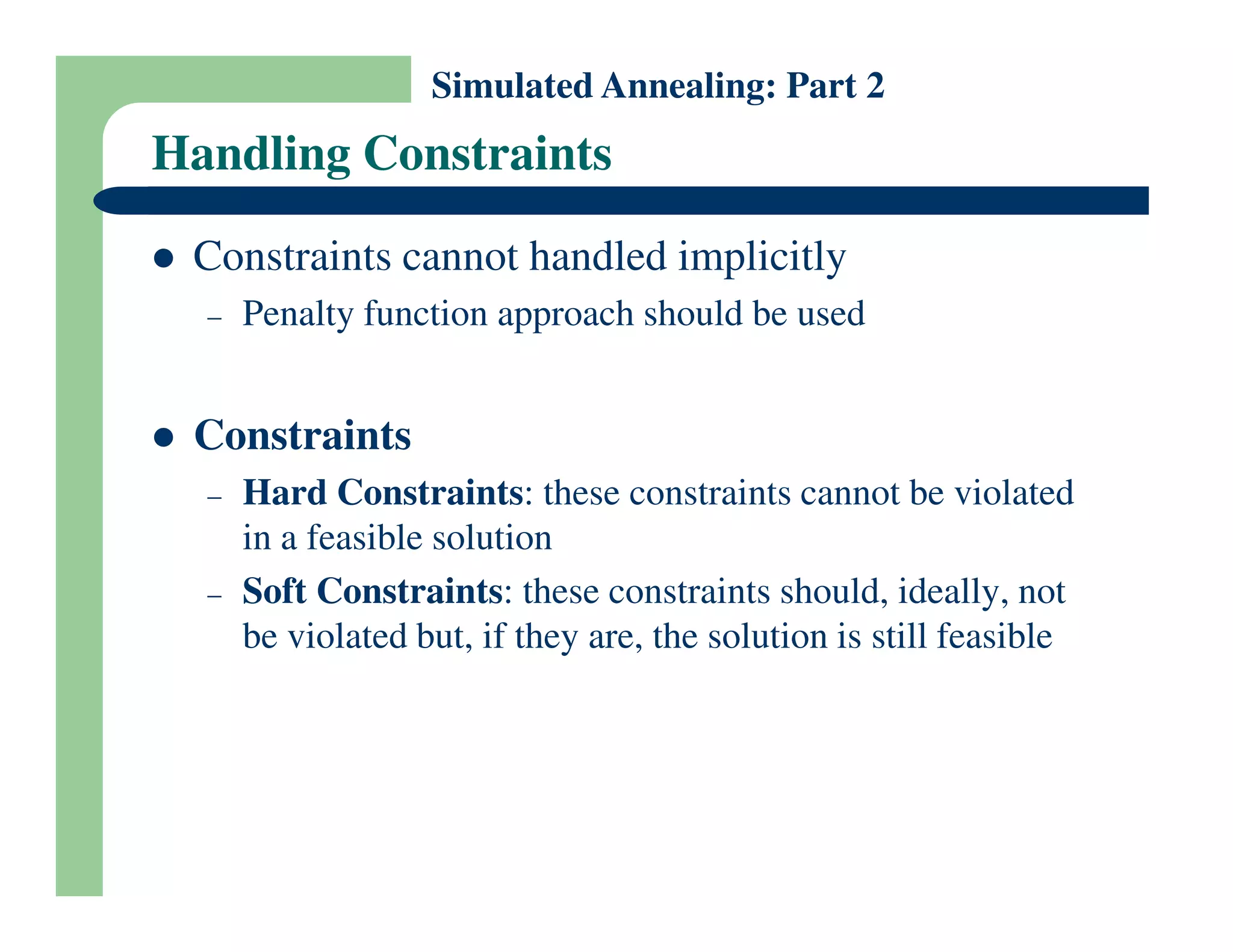
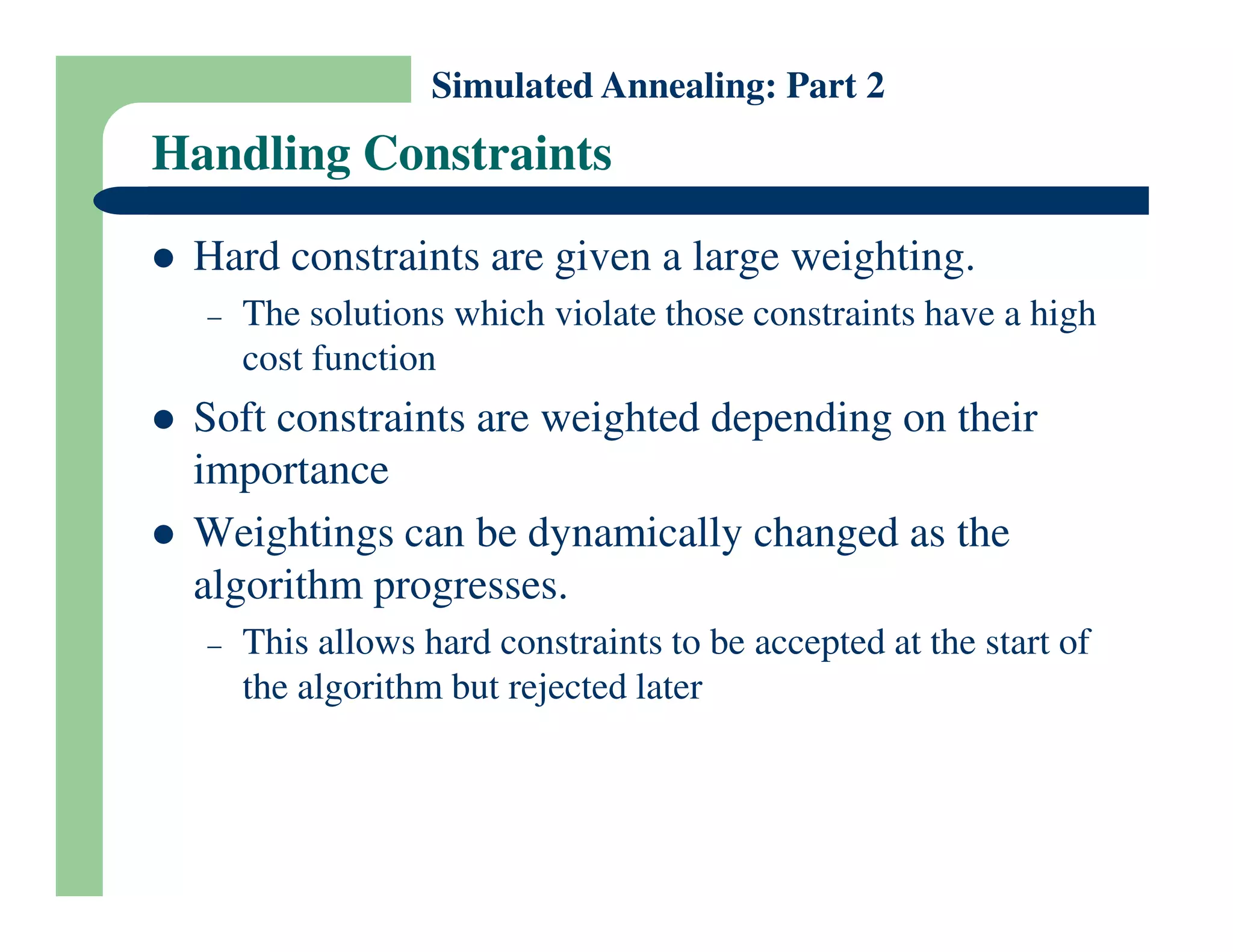


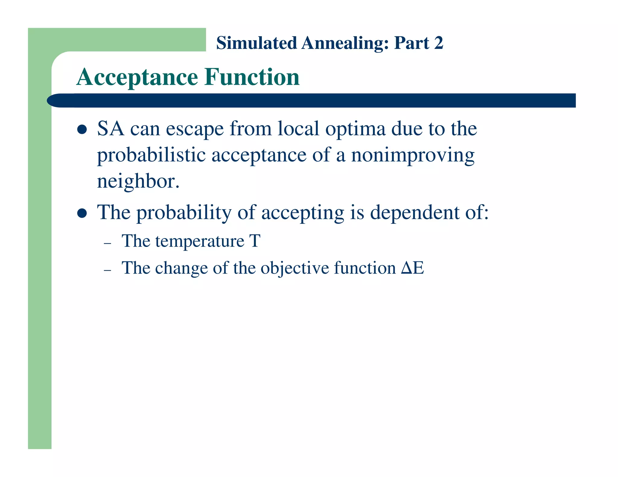
This document discusses various concepts related to simulated annealing including the acceptance function, initial temperature, equilibrium state, cooling schedule, stopping condition, and handling constraints. It describes how the acceptance of non-improving moves is based on temperature and change in objective function. It also provides examples of different cooling schedules and discusses how to determine equilibrium state and stopping criteria. The document concludes with applying simulated annealing to solve the knapsack problem.