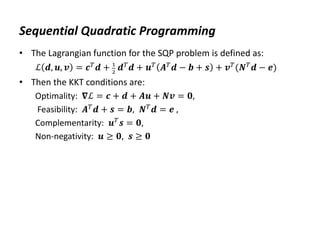
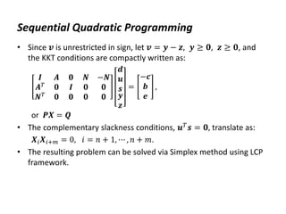
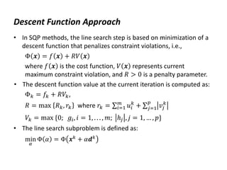
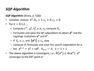
The document discusses various numerical optimization methods for solving unconstrained nonlinear problems. It covers iterative methods for finding the optimal solution, including techniques for determining a suitable search direction and performing a line search to minimize the objective function along that direction. Specific methods covered include the steepest descent method, conjugate gradient method, Newton's method, trust region methods, and line search techniques like the golden section search and quadratic approximation.


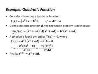
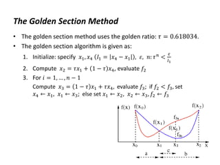
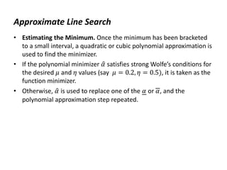
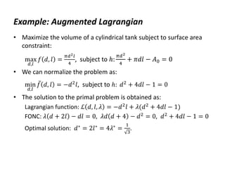
![Example: Approximate Search
• Let 𝑓 𝛼 = 𝑒−𝛼 + 𝛼2, 𝑓′ 𝛼 = 2𝛼 − 𝑒−𝛼, 𝑓 0 = 1, 𝑓′ 0 = −1.
Let 𝜇 = 0.2, and try 𝛼 = 0.1, 0.2, …, to bracket the minimum.
• From the sufficient decrease condition, the minimum is bracketed
in the interval: [0, 0.5]
• Using quadratic approximation, the minimum is found as:
𝑥∗
= 0.3531
The exact solution is given as: 𝛼𝑚𝑖𝑛 = 0.3517
• The Matlab commands are:
Define the function:
f=@(x) x.*x+exp(-x);
mu=0.2; al=0:.1:1;](https://image.slidesharecdn.com/optimumengineeringdesign-day5-240221195559-b78ed600/85/Optimum-engineering-design-Day-5-Clasical-optimization-methods-16-320.jpg)
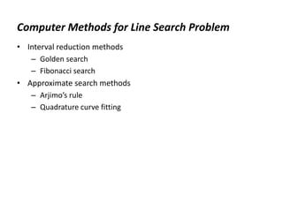
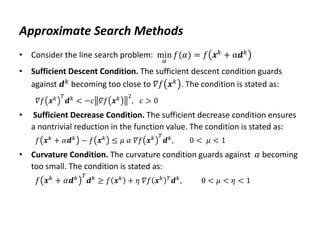
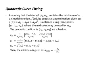
![Example: Steepest Descent
• MATLAB code:
H=[.2 0;0 2];
f=@(x) x'*H*x/2; df=@(x) H*x; ddf=H;
x=[5;1];
xall=x';
for i=1:10
d=-df(x);
a=d'*d/(d'*H*d);
x=x+a*d;
xall=[xall;x'];
end
plot(xall(:,1),xall(:,2)), grid
axis([-1 5 -1 5]), axis equal](https://image.slidesharecdn.com/optimumengineeringdesign-day5-240221195559-b78ed600/85/Optimum-engineering-design-Day-5-Clasical-optimization-methods-22-320.jpg)
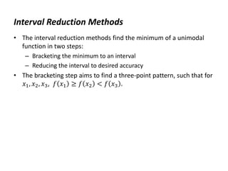
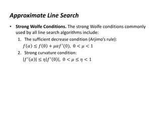
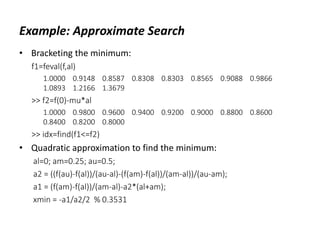
![Example: Conjugate Gradient Method
• MATLAB code
H=[.2 0;0 2];
f=@(x) x'*H*x/2; df=@(x) H*x; ddf=H;
x=[5;1]; n=2;
xall=zeros(n+1,n); xall(1,:)=x';
d=-df(x); a=d'*d/(d'*H*d);
x=x+a*d; xall(2,:)=x';
for i=1:size(x,1)-1
b=df(x)'*H*d/(d'*H*d);
d=-df(x)+b*d;
r=-df(x);
a=r'*r/(d'*H*d);
x=x+a*d;
xall(i+2,:)=x';
end
plot(xall(:,1),xall(:,2)), grid
axis([-1 5 -1 5]), axis equal](https://image.slidesharecdn.com/optimumengineeringdesign-day5-240221195559-b78ed600/85/Optimum-engineering-design-Day-5-Clasical-optimization-methods-28-320.jpg)
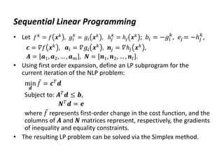
![SLP Example
• Consider the convex NLP problem:
min
𝑥1,𝑥2
𝑓(𝑥1, 𝑥2) = 𝑥1
2
− 𝑥1𝑥2 + 𝑥2
2
Subject to: 1 − 𝑥1
2
− 𝑥2
2
≤ 0; −𝑥1 ≤ 0, −𝑥2 ≤ 0
The problem has a single minimum at: 𝒙∗
=
1
2
,
1
2
• The objective and constraint gradients are:
𝛻𝑓𝑇
= 2𝑥1 − 𝑥2, 2𝑥2 − 𝑥1 ,
𝛻𝑔1
𝑇
= −2𝑥1, −2𝑥2 , 𝛻𝑔2
𝑇
= −1,0 , 𝛻𝑔3
𝑇
= [0, −1].
• Let 𝒙0
= 1, 1 , then 𝑓0
= 1, 𝒄𝑇
= 1 1 , 𝑏1 = 𝑏2 = 𝑏3 = 1;
𝒂1
𝑇
= −2 − 2 , 𝒂2
𝑇
= −1 0 , 𝒂3
𝑇
= 0 − 1](https://image.slidesharecdn.com/optimumengineeringdesign-day5-240221195559-b78ed600/85/Optimum-engineering-design-Day-5-Clasical-optimization-methods-54-320.jpg)
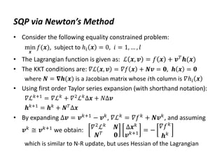
![SQP Example
• Consider the NLP problem: min
𝑥1,𝑥2
𝑓(𝑥1, 𝑥2) = 𝑥1
2
− 𝑥1𝑥2 + 𝑥2
2
subject to 𝑔1: 1 − 𝑥1
2
− 𝑥2
2
≤ 0, 𝑔2: −𝑥1 ≤ 0, 𝑔3: −𝑥2 ≤ 0
Then 𝛻𝑓𝑇
= 2𝑥1 − 𝑥2, 2𝑥2 − 𝑥1 , 𝛻𝑔1
𝑇
= −2𝑥1, −2𝑥2 , 𝛻𝑔2
𝑇
=
−1,0 , 𝛻𝑔3
𝑇
= [0, −1]. Let 𝑥0 = 1, 1 ; then, 𝑓0 = 1, 𝒄 = 1, 1 𝑇,
𝑔1 1,1 = 𝑔2 1,1 = 𝑔3 1,1 = −1.
• Since all constraints are initially inactive, 𝑉0 = 0, and 𝒅 = −𝒄 =
−1, −1 𝑇; the line search problem is: min
𝛼
Φ 𝛼 = 1 − 𝛼 2;
• By setting Φ′
𝛼 = 0, we get the analytical solution: 𝛼 = 1; thus
𝑥1 = 0, 0 , which results in a large constraint violation](https://image.slidesharecdn.com/optimumengineeringdesign-day5-240221195559-b78ed600/85/Optimum-engineering-design-Day-5-Clasical-optimization-methods-63-320.jpg)
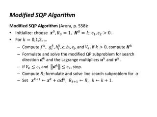
![Example: SQP with Hessian Update
• Consider the NLP problem: min
𝑥1,𝑥2
𝑓(𝑥1, 𝑥2) = 𝑥1
2
− 𝑥1𝑥2 + 𝑥2
2
subject to 𝑔1: 1 − 𝑥1
2
− 𝑥2
2
≤ 0, 𝑔2: −𝑥1 ≤ 0, 𝑔3: −𝑥2 ≤ 0
Let 𝑥0
= 1, 1 ; then, 𝑓0
= 1, 𝒄 = 1, 1 𝑇
, 𝑔1 1,1 = 𝑔2 1,1 =
𝑔3 1,1 = −1; 𝛻𝑔1
𝑇
= −2, −2 , 𝛻𝑔2
𝑇
= −1,0 , 𝛻𝑔3
𝑇
= [0, −1].
• Using approximate line search, 𝛼 =
1
4
, 𝒙1 =
3
4
,
3
4
.
• For the Hessian update, we have:
𝑓1 = 0.5625, 𝑔1 = −0.125, 𝑔2 = 𝑔3 = −0.75; 𝒄1 = [0.75, 0.75];
𝛻𝑔1
𝑇
= −
3
2
, −
3
2
, 𝛻𝑔2
𝑇
= −1,0 , 𝛻𝑔3
𝑇
= 0, −1 ; Δ𝒙0
= −0.25, −0.25 ;
then, 𝑫0 = 8
1 1
1 1
, 𝑬0 = 8
1 1
1 1
, 𝑯1 = 𝑯0](https://image.slidesharecdn.com/optimumengineeringdesign-day5-240221195559-b78ed600/85/Optimum-engineering-design-Day-5-Clasical-optimization-methods-68-320.jpg)
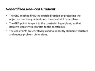
![SQP Algorithm
%SQP subproblem via Hessian update
% input: xk (current design); Lk (Hessian of Lagrangian
estimate)
%initialize
n=size(xk,1);
if ~exist('Lk','var'), Lk=diag(xk+(~xk)); end
tol=1e-7;
%function and constraint values
fk=f(xk);
dfk=df(xk);
gk=g(xk);
dgk=dg(xk);
%N-R update
A=[Lk dgk; dgk' 0*dgk'*dgk];
b=[-dfk;-gk];
dx=Ab;
dxk=dx(1:n);
lam=dx(n+1:end);](https://image.slidesharecdn.com/optimumengineeringdesign-day5-240221195559-b78ed600/85/Optimum-engineering-design-Day-5-Clasical-optimization-methods-71-320.jpg)
![SQP Algorithm
%inactive constraints
idx1=find(lam<0);
if idx1
[dxk,lam]=inactive(lam,A,b,n);
end
%check termination
if abs(dxk)<tol, return, end
%adjust increment for constraint compliance
P=@(xk) f(xk)+lam'*abs(g(xk));
while P(xk+dxk)>P(xk),
dxk=dxk/2;
if abs(dxk)<tol, break, end
end
%Hessian update
dL=@(x) df(x)+dg(x)*lam;
Lk=update(Lk, xk, dxk, dL);
xk=xk+dxk;
disp([xk' f(xk) P(xk)])](https://image.slidesharecdn.com/optimumengineeringdesign-day5-240221195559-b78ed600/85/Optimum-engineering-design-Day-5-Clasical-optimization-methods-72-320.jpg)
![SQP Algorithm
%function definitions
function [dxk,lam]=inactive(lam,A,b,n)
idx1=find(lam<0);
lam(idx1)=0;
idx2=find(lam);
v=[1:n,n+idx2];
A=A(v,v); b=b(v);
dx=Ab;
dxk=dx(1:n);
lam(idx2)=dx(n+1:end);
end
function Lk=update(Lk, xk, dxk, dL)
ga=dL(xk+dxk)-dL(xk);
Hx=Lk*dxk;
Dk=ga*ga'/(ga'*dxk);
Ek=Hx*Hx'/(Hx'*dxk);
Lk=Lk+Dk-Ek;
end](https://image.slidesharecdn.com/optimumengineeringdesign-day5-240221195559-b78ed600/85/Optimum-engineering-design-Day-5-Clasical-optimization-methods-73-320.jpg)
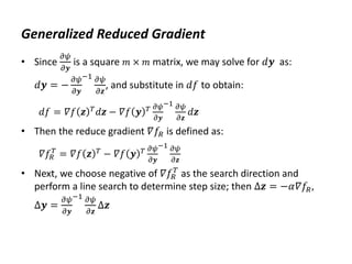
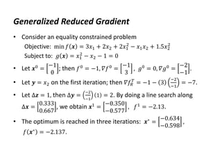
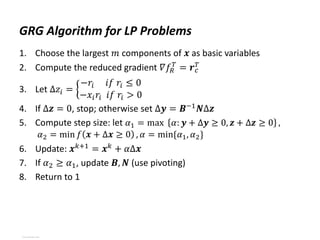
![Generalized Reduced Gradient
• Let 𝑦 = 𝑥1, 𝒛 =
𝑥2
𝑠2
; then 𝛻𝑓 𝑦 = 5.12, 𝛻𝑓 𝒛 =
1
0
, 𝛻𝑔2 𝑦 = 1,
𝛻𝑔2 𝒛 =
1
1
, therefore 𝛻𝑓𝑅 𝒛 =
1
0
−
1
1
5.12 =
−4.12
−5.12
• Let Δ𝒛 = −𝛻𝑓𝑅 𝒛 , Δ𝑦 = −[1 1]Δ𝒛 = −9.24; then, Δ𝒙 =
−9.24
4.12
and
𝒔0 = Δ𝒙/ Δ𝒙 . Suppose we limit the maximum step size to 𝛼 ≤ 0.5,
then 𝒙1 = 𝒙0 + 0.5𝒔0 =
2.103
−1.356
with 𝑓 𝑥1 = 𝑓1 = 3.068. There are
no constraint violations, hence first iteration is completed.
• After seven iterations: 𝒙7 =
0.003
−3.0
with 𝑓7 = −3.0
• The optimum is at: 𝒙∗ =
0.0
−3.0
with 𝑓∗ = −3.0](https://image.slidesharecdn.com/optimumengineeringdesign-day5-240221195559-b78ed600/85/Optimum-engineering-design-Day-5-Clasical-optimization-methods-81-320.jpg)
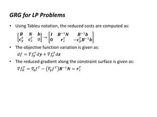
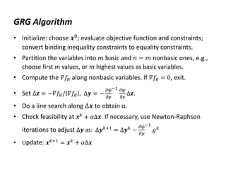
![GRG for LP Problems
• Consider an LP problem: min 𝑓(𝒙) = 𝒄𝑇
𝒙
Subject to: 𝑨𝒙 = 𝒃, 𝒙 ≥ 𝟎
• Let 𝒙 be partitioned into 𝑚 basic variables and 𝑛 − 𝑚 nonbasic
variables: 𝒙𝑇
= [𝒚𝑇
, 𝒛𝑇
].
• The objective function is partitioned as: 𝑓 𝒙 = 𝒄𝑦
𝑇
𝒚 + 𝒄𝑧
𝑇
𝒛
• The constraints are partitioned as: 𝑩𝒚 + 𝑵𝒛 = 𝒃, 𝒚 ≥ 𝟎, 𝒛 ≥ 𝟎.
Then 𝒚 = 𝑩−1𝒃 − 𝑩−1𝑵𝒛
• The objective function in terms of independent variables is:
𝑓 𝒛 = 𝒄𝑦
𝑇
𝑩−1
𝒃𝒛 + (𝒄𝑧
𝑇
− 𝒄𝑦
𝑇
𝑩−1
𝑵)𝒛
• The reduced costs for nonbasic variables are given as:
𝒓𝑐
𝑇
= 𝒄𝑧
𝑇
− 𝒄𝑦
𝑇
𝑩−1
𝑵, or 𝒓𝑐
𝑇
= 𝒄𝑧
𝑇
− 𝝀𝑇
𝑵](https://image.slidesharecdn.com/optimumengineeringdesign-day5-240221195559-b78ed600/85/Optimum-engineering-design-Day-5-Clasical-optimization-methods-82-320.jpg)