Downloaded 78 times

![Structural Cracking, faulting, raveling, etc.
Functional Riding comfort (measured in terms of
roughness of pavement.)
Serviceability Performance: Measured by PSI Present
Serviceability Index with scale 0 to 5.
0 "Road closed"
5 "Just constructed" Initial PSI (pi) [4.2 (rigid)
and 4.5(flexible)]
Terminal PSI (pt)
2.5 to 3.0 for major highways
2.0 for lower class highways
1.5 for very special cases
PSI
Serviceability (contd.)](https://image.slidesharecdn.com/termpaperce690-130511132342-phpapp01/75/Critical-Appraisal-of-Pavement-Design-of-Ohio-Department-of-Transportation-ODOT-7-2048.jpg)


![Use of layer coefficients a1, a2 and a3
The approach of use of layer coefficients has been found
to be inappropriate for design purposes [Coree and
White (1990)]
The layer coefficient has been found to be NOT a simple
function of the individual layer modulus, but a function
of all layer thicknesses and properties. [Baladi and
Thomas (1994)]](https://image.slidesharecdn.com/termpaperce690-130511132342-phpapp01/75/Critical-Appraisal-of-Pavement-Design-of-Ohio-Department-of-Transportation-ODOT-24-2048.jpg)


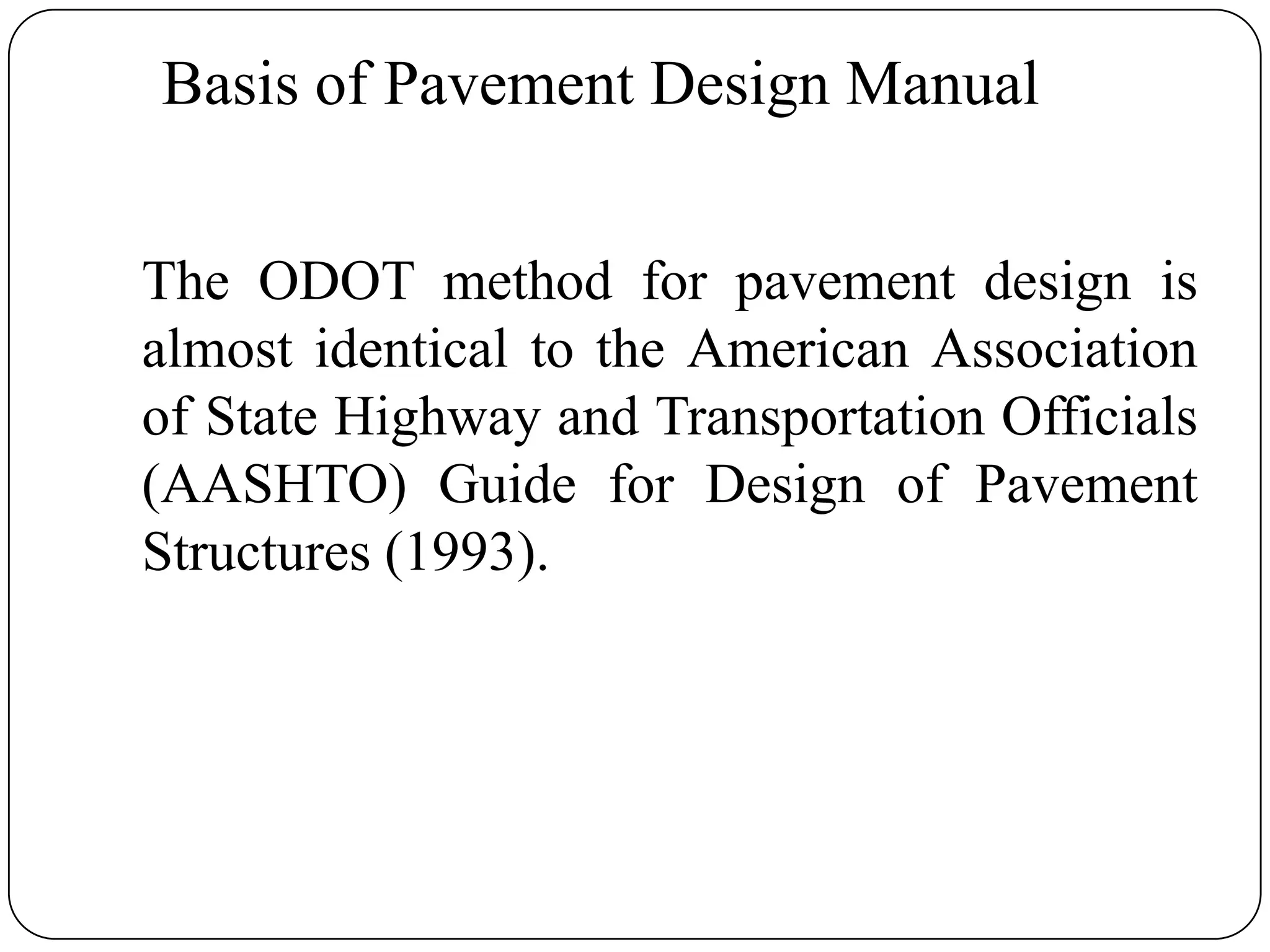
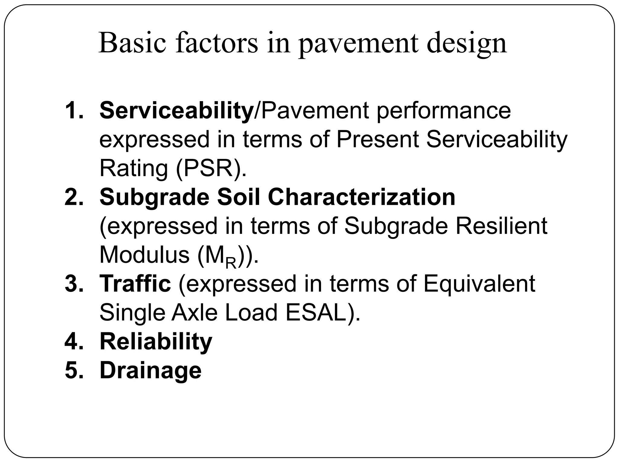
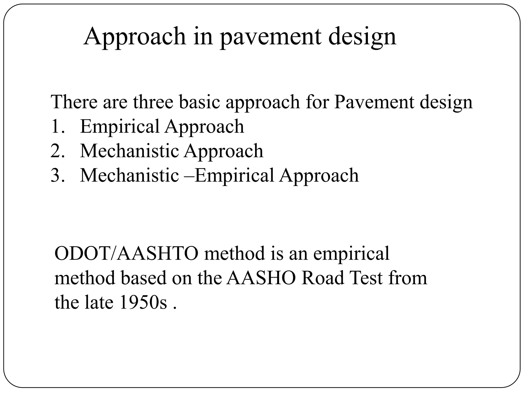
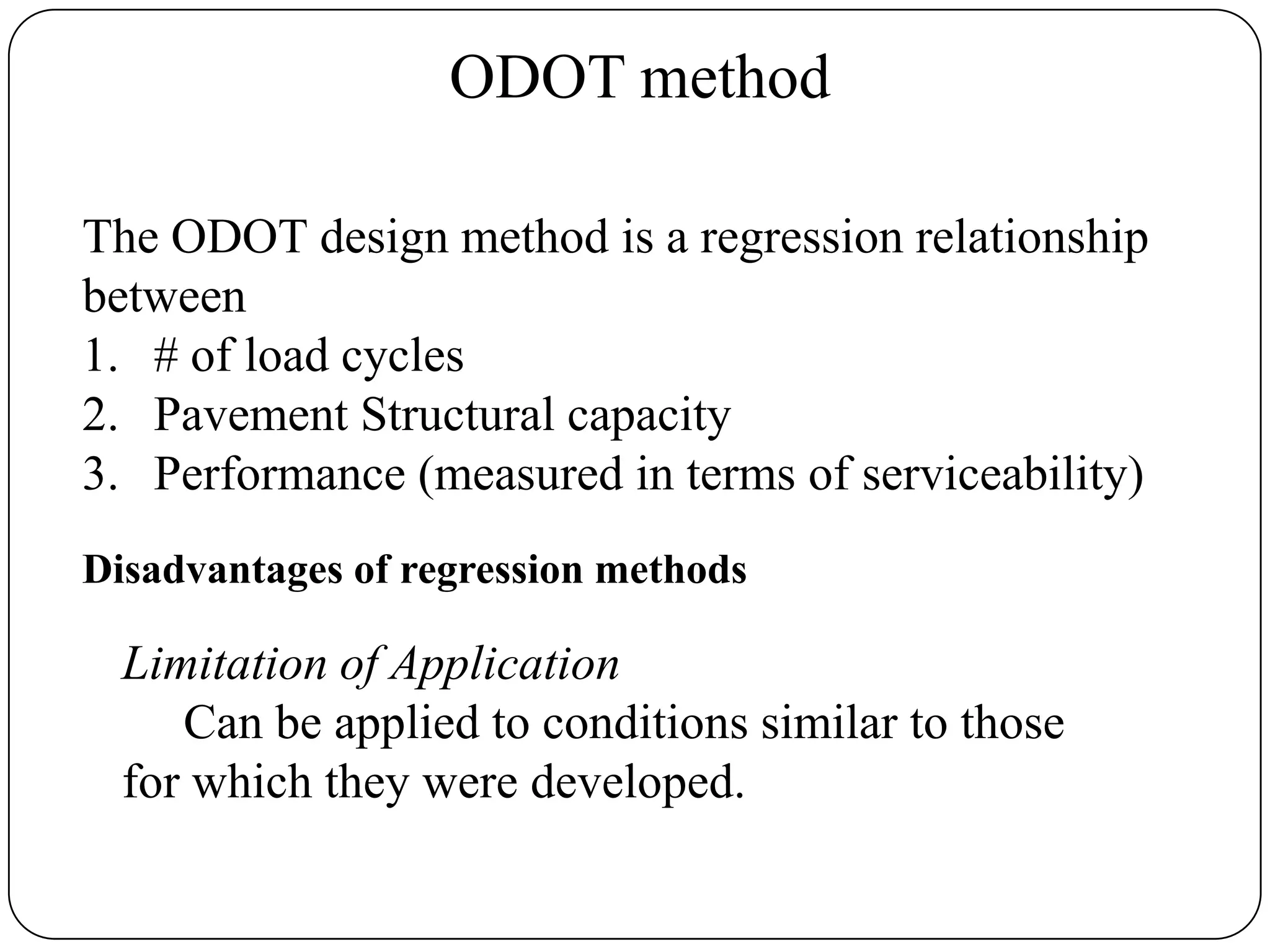
This document provides an overview of the Ohio Department of Transportation's (ODOT) pavement design method. It discusses the basic factors considered in design, including serviceability, subgrade characterization, traffic loading, reliability, and drainage. The ODOT method is based on the American Association of State Highway and Transportation Officials (AASHTO) Guide, using a regression relationship between load cycles, pavement structural capacity, and performance. It considers traffic loads in terms of equivalent single axle loads and uses reliability levels depending on road importance. Rigid and flexible pavement designs are outlined, including parameters considered and thickness design processes. Limitations of the current ODOT method are also discussed.


![Geotechnical Engineering-I [Lec #1: Introduction]](https://cdn.slidesharecdn.com/ss_thumbnails/1-180923175052-thumbnail.jpg?width=640&height=640&fit=bounds)
![Geotechnical Engineering-I [Lec #18: Consolidation-II]](https://cdn.slidesharecdn.com/ss_thumbnails/18-180924140946-thumbnail.jpg?width=640&height=640&fit=bounds)


![Geotechnical Engineering-II [Lec #7A: Boussinesq Method]](https://cdn.slidesharecdn.com/ss_thumbnails/7a-181020124807-thumbnail.jpg?width=640&height=640&fit=bounds)


![Geotechnical Engineering-I [Lec #17: Consolidation]](https://cdn.slidesharecdn.com/ss_thumbnails/17-180924140731-thumbnail.jpg?width=640&height=640&fit=bounds)


![Geotechnical Engineering-I [Lec #21: Consolidation Problems]](https://cdn.slidesharecdn.com/ss_thumbnails/21-180924141121-thumbnail.jpg?width=640&height=640&fit=bounds)


![Geotechnical Engineering-II [Lec #7: Soil Stresses due to External Load]](https://cdn.slidesharecdn.com/ss_thumbnails/7-180930132739-thumbnail.jpg?width=640&height=640&fit=bounds)


![Geotechnical Engineering-II [Lec #9+10: Westergaard Theory]](https://cdn.slidesharecdn.com/ss_thumbnails/9-181020124827-thumbnail.jpg?width=640&height=640&fit=bounds)


![Geotechnical Engineering-II [Lec #27: Infinite Slope Stability Analysis]](https://cdn.slidesharecdn.com/ss_thumbnails/27-181125070251-thumbnail.jpg?width=640&height=640&fit=bounds)