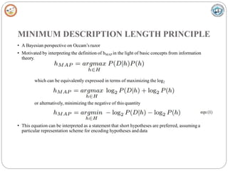
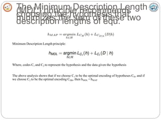
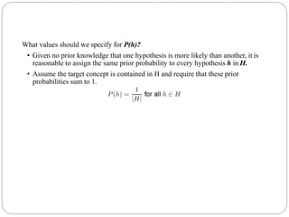
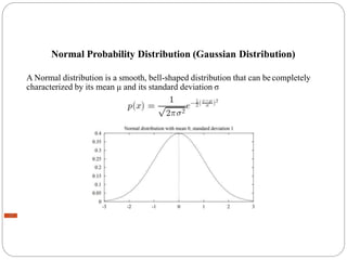
Bayesian learning methods calculate explicit probabilities for hypotheses. They allow each training example to incrementally increase or decrease a hypothesis' probability. Prior knowledge can be combined with data to determine final probabilities. Bayesian methods can accommodate probabilistic hypotheses and classify instances by combining hypothesis predictions weighted by probabilities. The minimum description length principle provides a Bayesian perspective on Occam's razor, preferring shorter hypotheses that minimize description length.

1. || Jai Sri Gurudev||
Sri Adichunchanagiri Shikshana Trust (R)
SJB INSTITUTE OF TECHNOLOGY
(Affiliated to Visvesvaraya Technological University, Belagavi& Approved by AICTE, New Delhi.)
No. 67, BGS Health & Education City, Dr. Vishnuvardhan Road Kengeri, Bengaluru – 560 060
Subject: AI & ML(18CS71)
By
Supriya B N, Asst. professor,
Semester/Section: VII
Department of Information Science & Engineering
Aca. Year: ODD SEM /2021-22

2. Bayesian Learning
• Introduction to Bayesian.
• Bayes theorem.
• Bayes theorem and concept learning.
• MDL principle.
• Bayesian belief networks
• EM algorithm
2 Dept. of ISE, SJBIT

3. INTRODUCTION
Bayesian learning methods are relevant to study of machine learning for two
different reasons.
• First, Bayesian learning algorithms that calculate explicit probabilities for
hypotheses, such as the naive Bayes classifier, are among the most practical
approaches to certain types of learning problems
• The second reason is that they provide a useful perspective for understanding
many learning algorithms that do not explicitly manipulate probabilities.

4. Features of Bayesian Learning Methods
• Each observed training example can incrementally decrease or increase the estimated
probability that a hypothesis is correct. This provides a more flexible approach to
learning than algorithms that completely eliminate a hypothesis if it is found to be
inconsistent with any single example
• Prior knowledge can be combined with observed data to determine the final
probability of a hypothesis. In Bayesian learning, prior knowledge is provided by
asserting (1) a prior probability for each candidate hypothesis, and (2) a probability
distribution over observed data for each possible hypothesis.
• Bayesian methods can accommodate hypotheses that make probabilistic predictions
• New instances can be classified by combining the predictions of multiple hypotheses,
weighted by their probabilities.
• Even in cases where Bayesian methods prove computationally intractable, they can
provide a standard of optimal decision making against which other practical methods
can be measured.

5. Practical difficulty in applying Bayesian methods
• One practical difficulty in applying Bayesian methods is that they typically require
initial knowledge of many probabilities. When these probabilities are not known
in advance they are often estimated based on background knowledge, previously
available data, and assumptions about the form of the underlying distributions.
• A second practical difficulty is the significant computational cost required to
determine the Bayes optimal hypothesis in the general case. In certain specialized
situations, this computational cost can be significantly reduced.

6. BAYESTHEOREM
Bayes theorem provides a way to calculate the probability of a hypothesis based on
its prior probability, the probabilities of observing various data given the hypothesis,
and the observed data itself.
Notations
• P(h) prior probability of h, reflects any background knowledge about the chance
that h is correct
• P(D) prior probability of D, probability that D will be observed
• P(D|h) probability of observing D given a world in which h holds
• P(h|D) posterior probability of h, reflects confidence that h holds after D has been
observed

7. Bayes theorem is the cornerstone of Bayesian learning methods because it
provides a way to calculate the posterior probability P(h|D), from the prior
probability P(h), together with P(D) and P(D(h).
P(h|D) increases with P(h) and with P(D|h) according to Bayes theorem.
P(h|D) decreases as P(D) increases, because the more probable it is that D will be
observed independent of h, the less evidence D provides in support of h.

8. Maximum a Posteriori (MAP) Hypothesis
• In many learning scenarios, the learner considers some set of candidate hypotheses
H and is interested in finding the most probable hypothesis h ∈
H given the
observed data D. Any such maximally probable hypothesis is called a maximum a
posteriori (MAP) hypothesis.
• Bayes theorem to calculate the posterior probability of each candidate hypothesis is hMAP
is a MAP hypothesis provided
• P(D) can be dropped, because it is a constant independent of h

9. Maximum Likelihood (ML) Hypothesis
In some cases, it is assumed that every hypothesis in H is equally probable a priori
(P(hi) = P(hj) for all hi and hj inH).
In this case the below equation can be simplified and need only consider the term
P(D|h) to find the most probable hypothesis.
P(D|h) is often called the likelihood of the data D given h, and any hypothesis that
maximizes P(D|h) is called a maximum likelihood (ML) hypothesis

10. Example
Consider a medical diagnosis problem in which there are two alternative hypotheses
• The patient has a particular form of cancer (denoted by cancer)
• The patient does not (denoted by ¬ cancer)
The available data is from a particular laboratory with two possible outcomes: +
(positive) and - (negative)

11. • Suppose a new patient is observed for whom the lab test returns a positive (+)
result.
• Should we diagnose the patient as having cancer or not?

12. BAYESTHEOREM AND CONCEPTLEARNING
What is the relationship between Bayes theorem and the problem of concept
learning?
Since Bayes theorem provides a principled way to calculate the posterior probability
of each hypothesis given the training data, and can use it as the basis for a
straightforward learning algorithm that calculates the probability for each possible
hypothesis, then outputs the most probable.

13. Brute-Force Bayes Concept Learning
We can design a straightforward concept learning algorithm to output the maximum
a posteriori hypothesis, based on Bayes theorem, as follows:

14. In order specify a learning problem for the BRUTE-FORCE MAP
LEARNING
algorithm we must specify what values are to be used for P(h) and for
P(D|h) ?
Lets choose P(h) and for P(D|h) to be consistent with the following assumptions:
• The training data D is noise free (i.e., di = c(xi))
• The target concept c is contained in the hypothesis space H
• We have no a priori reason to believe that any hypothesis is more probable than any other.

15. What values should we specify for P(h)?
• Given no prior knowledge that one hypothesis is more likely than another, it is
reasonable to assign the same prior probability to every hypothesis h in H.
• Assume the target concept is contained in H and require that these prior
probabilities sum to 1.

16. What choice shall we make for P(D|h)?
• P(D|h) is the probability of observing the target values D = (d1 . . .dm) for the
fixed set of instances (x1 . . . xm), given a world in which hypothesis hholds
• Since we assume noise-free training data, the probability of observing
classification di given h is just 1 if di = h(xi) and 0 if di# h(xi). Therefore,

17. Given these choices for P(h) and for P(D|h) we now have
a fully-defined problem for the above BRUTE-FORCE
MAP LEARNING algorithm.
In a first step, we have to determine the probabilities for P(h|D)

18. To summarize, Bayes theorem implies that the posterior probability
P(h|D) under our assumed P(h) and P(D|h) is
where |VSH,D| is the number of hypotheses from H consistent with D

19. The Evolution of Probabilities Associated with Hypotheses
• Figure (a) all hypotheses have the same probability.
• Figures (b) and (c), As training data accumulates, the posterior probability for
inconsistent hypotheses becomes zero while the total probability summing to 1 is
shared equally among the remaining consistent hypotheses.

20. MAP Hypotheses and Consistent Learners
A learning algorithm is a consistent learner if it outputs a hypothesis that commits zero errors over the
training examples.
Every consistent learner outputs a MAP hypothesis, if we assume a uniform prior probability
distribution over H (P(hi) = P(hj) for all i, j), and deterministic, noise free training data (P(D|h) =1 if
D and h are consistent, and 0 otherwise).
Example:
• FIND-S outputs a consistent hypothesis, it will output a MAP hypothesis under the probability
distributions P(h) and P(D|h) defined above.
• Are there other probability distributions for P(h) and P(D|h) under which FIND-S outputs MAP
hypotheses? Yes.
• Because FIND-S outputs a maximally specific hypothesis from the version space, its output
hypothesis will be a MAP hypothesis relative to any prior probability distribution that favours more
specific hypotheses.

21. • Bayesian framework is a way to characterize the behaviour of learning algorithms
• By identifying probability distributions P(h) and P(D|h) under which the output is
a optimal hypothesis, implicit assumptions of the algorithm can be characterized
(Inductive Bias)
• Inductive inference is modelled by an equivalent probabilistic reasoning system
based on Bayes theorem

22. MAXIMUM LIKELIHOOD AND LEAST-SQUARED
ERROR HYPOTHESES
Consider the problem of learning a continuous-valued target function such as neural
network learning, linear regression, and polynomial curve fitting
A straightforward Bayesian analysis will show that under certain assumptions any
learning algorithm that minimizes the squared error between the output hypothesis
predictions and the training data will output a maximum likelihood (ML) hypothesis

23. Learning A Continuous-Valued TargetFunction
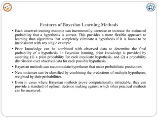
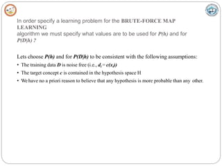
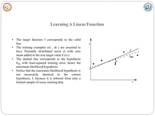
• Learner L considers an instance space X and a hypothesis space H consisting of some class ofreal-
valued functions defined over X, i.e., (∀ h ∈
H)[ h : X → R] and training examples of theform
<xi,di>
• The problem faced by L is to learn an unknown target function f : X →R
• A set of m training examples is provided, where the target value of each example is corruptedby
random noise drawn according to a Normal probability distribution with zero mean (di = f(xi) + ei)
• Each training example is a pair of the form (xi ,di ) where di = f (xi ) + ei .
– Here f(xi) is the noise-free value of the target function and ei is a random variable representing
the noise.
–It is assumed that the values of the ei are drawn independently and that they are distributed
according to a Normal distribution with zero mean.
• The task of the learner is to output a maximum likelihood hypothesis, or, equivalently, aMAP
hypothesis assuming all hypotheses are equally probable a priori.

24. Learning A LinearFunction
• The target function f corresponds to the solid
line.
• The training examples (xi , di ) are assumed to
have Normally distributed noise ei with zero
mean added to the true target value f (xi ).
• The dashed line corresponds to the hypothesis
hML with least-squared training error, hence the
maximum likelihood hypothesis.
• Notice that the maximum likelihood hypothesis is
not necessarily identical to the correct
hypothesis, f, because it is inferred from only a
limited sample of noisy training data

25. Before showing why a
hypothesis that minimizes the
sum of squared errors in this
setting is also a maximum
likelihood hypothesis, let us
quickly review probability
densities and Normal distributions
Probability Density for continuous variables
e: a random noise variable generated by a Normal probabilitydistribution
<x1 . . . xm>: the sequence of instances (asbefore)
<d1 . . . dm>: the sequence of target values with di = f(xi) + ei

26. Normal Probability Distribution (Gaussian Distribution)
A Normal distribution is a smooth, bell-shaped distribution that can be completely
characterized by its mean μ and its standard deviation σ
26

28. previous
definition of hML
we have
Assuming training examples are mutually independent given h, we can write P(D|h) as the product of
the various (di|h)
Given the noise ei obeys a Normal distribution with zero mean and unknown variance σ2 , each di
must also obey a Normal distribution around the true targetvalue f(xi). Because we are writing the
expression for P(D|h), we assume h is the correct description of f. Hence, µ = f(xi) =h(xi)

29. It is common to maximize the
less complicated logarithm,
which is justified because of
the monotonicity of function p.
The first term in this expression is a constant independent of h and can therefore bediscarded
Maximizing this negative term is equivalent to minimizing the corresponding positiveterm.

30. Finally Discard constants that are independent ofh
• the hML is one that minimizes the sum of the squared errors
Why is it reasonable to choose the Normal distribution to characterizenoise?
• good approximation of many types of noise in physical systems
• Central Limit Theorem shows that the sum of a sufficiently large number ofindependent,
identically distributed random variables itself obeys a Normal distribution
Only noise in the target value is considered, not in the attributes describing theinstances
themselves

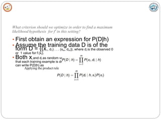
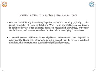
31. MAXIMUM LIKELIHOOD HYPOTHESES
FOR PREDICTING PROBABILITIES
Consider the setting in which we wish to learn a nondeterministic (probabilistic)
function f : X → {0, 1}, which has two discrete output values.
We want a function approximator whose output is the probability that f(x) = 1
In other words , learn the target function
f’ : X → [0, 1] such that f’(x) = P(f(x) = 1)
How can we learn f' using a neural network?
Use of brute force way would be to first collect the observed frequencies of 1's and
0's for each possible value of x and to then train the neural network to output the
target frequency for each x.

32. What criterion should we optimize in order to find a maximum
likelihood hypothesis for f' in this setting?
• First obtain an expression for P(D|h)
• Assume the training data D is of the
form D = {(x1, d1) . . . (xm, dm)}, where di is the observed 0
or 1 value for f (xi).
• Both xi and di as random variables, and assuming
that each training example is drawn independently, we
can write P(D|h) as
Applying the product rule

33. The probability P(di|h, xi)
Re-express it in a more mathematically manipulable form, as
Equation (4) to substitute for P(di |h, xi) in Equation (5) to obtain

34. We write an expression for the maximum likelihood hypothesis
The last term is a constant independent of h, so it can be dropped
It easier to work with the log of the likelihood, yielding
Equation (7) describes the quantity that must be maximized in order to obtain themaximum
likelihood hypothesis in our current problemsetting

35. Gradient Search to Maximize Likelihood in a Neural Net
Derive a weight-training rule for neural network learning that seeks to maximize G(h, D)using
gradient ascent
• The gradient of G(h, D) is given by the vector of partial derivatives of G(h, D) with respect tothe
various network weights that define the hypothesis h represented by the learnednetwork
• In this case, the partial derivative of G(h, D) with respect to weight wjk from input k to unit j is

36. Suppose our neural network is constructed from a single layer of sigmoid units. Then,
where xijk is the kth input to unit j for the ith training example, and d(x) is the derivative of the sigmoid
squashing function.
Finally, substituting this expression into Equation (1), we obtain a simple expression forthe
derivatives that constitute the gradient

37. Because we seek to maximize
rather than minimize P(D|h), we
perform gradient ascent rather than
gradient descent search. On each
iteration of the search the weight
vector is adjusted in the direction
of the gradient, using the weight
update rule
where η is a small positive constant that determines the step size of the i gradient ascent search

38. It is interesting to compare this weight-update rule to the weight-update rule used by the
BACKPROPAGATION algorithm to minimize the sum of squared errors between predicted and
observed network outputs.
The BACKPROPAGATION update rule for output unit weights, re-expressed using our current
notation, is

39. MINIMUM DESCRIPTION LENGTH PRINCIPLE
• A Bayesian perspective on Occam’s razor
• Motivated by interpreting the definition of hMAP in the light of basic concepts from information
theory.
which can be equivalently expressed in terms of maximizing the log2
or alternatively, minimizing the negative of this quantity
• This equation can be interpreted as a statement that short hypotheses are preferred, assuming a
particular representation scheme for encoding hypotheses and data

40. Introduction to a basic result of information theory
• Consider the problem of designing a code to transmit messages drawn at random
• i is the message
• The probability of encountering message i is pi
• Interested in the most compact code; that is, interested in the code that minimizes the
expected number of bits we must transmit in order to encode a message drawn at random
• To minimize the expected code length we should assign shorter codes to messages that are
more probable
• Shannon and Weaver (1949) showed that the optimal code (i.e., the code that minimizes
the expected message length) assigns - log, pi bitst to encode message i.
• The number of bits required to encode message i using code C as the description length
of message i with respect to C, which we denote by Lc(i).

41. ing the
equatio
n
• -log2P(h): the description length of h under the optimal encoding for the hypothesis space H
LCH (h) = −log2P(h), where CH is the optimal code for hypothesis space H.
• -log2P(D | h): the description length of the training data D given hypothesis h, under the
optimal encoding fro the hypothesis space H: LCH (D|h) = −log2P(D| h) , where C D|h is the
optimal code for describing data D assuming that both the sender and receiver know the
hypothesis h.
Rewrite Equation (1) to show that hMAP is the hypothesis h that minimizes the sum given by the
description length of the hypothesis plus the description length of the data given thehypothesis.
where CH and CD|h are the optimal encodings for H and for D given h

42. The Minimum Description Length
(MDL) principle recommends
choosing the hypothesis that
minimizes the sum of these two
description lengths of equ.
Minimum Description Length principle:
Where, codes C1 and C2 to represent the hypothesis and the data given the hypothesis
The above analysis shows that if we choose C1 to be the optimal encoding of hypotheses CH, and if
we choose C2 to be the optimal encoding CD|h, then hMDL = hMAP

43. References/Bibliography
Dept. of ISE, SJBIT
43
1) Machine Learning by Tom M. Mitchell, McGraw Hill India.
2) Introduction to machine learning by Ethem Alpaydın, MIT press second edition.