MACHINE LEARNING
Introduction To
Complete Guide
www.genial-code.com
▪ AAAI. Machine Learning.
http://www.aaai.org/Pathfinder/html/machine.html
▪ Dietterich,T. (2003). Machine Learning.Nature Encyclopedia of Cognitive
Science.
▪ Doyle, P. Machine Learning.
http://www.cs.dartmouth.edu/~brd/Teaching/AI/Lectures/Summaries/learn
ing.html
▪ Dyer, C. (2004). Machine Learning.
http://www.cs.wisc.edu/~dyer/cs540/notes/learning.html
▪ Mitchell,T. (1997). Machine Learning.
▪ Nilsson, N. (2004). Introduction to Machine Learning.
http://robotics.stanford.edu/people/nilsson/mlbook.html
▪ Russell, S. (1997). Machine Learning. Handbook of Perception and
Cognition,Vol. 14, Chap. 4.
▪ Russell, S. (2002). Artificial Intelligence:A Modern Approach, Chap. 18-20.
http://aima.cs.berkeley.edu
▪ “Learning denotes changes in a system that ...enable a
system to do the same task … more efficiently the next
time.” - Herbert Simon
▪ “Learning is constructing or modifying representations of
what is being experienced.”- Ryszard Michalski
▪ “Learning is making useful changes in our minds.”- Marvin
Minsky
“Machine learning refers to a system capable of the
autonomous acquisition and integration of knowledge.”
▪ No human experts
▪ industrial/manufacturing control
▪ mass spectrometer analysis, drug design, astronomic discovery
▪ Black-box human expertise
▪ face/handwriting/speech recognition
▪ driving a car, flying a plane
▪ Rapidly changing phenomena
▪ credit scoring, financial modeling
▪ diagnosis, fraud detection
▪ Need for customization/personalization
▪ personalized news reader
▪ movie/book recommendation
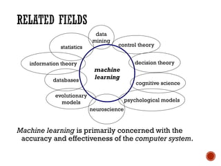
Machine learning is primarily concerned with the
accuracy and effectiveness of the computer system.
psychological models
data
mining
cognitive science
decision theory
information theory
databases
machine
learning
neuroscience
statistics
evolutionary
models
control theory
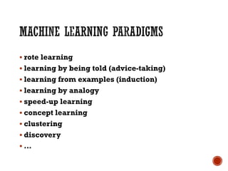
▪ rote learning
▪ learning by being told (advice-taking)
▪ learning from examples (induction)
▪ learning by analogy
▪ speed-up learning
▪ concept learning
▪ clustering
▪ discovery
▪ …
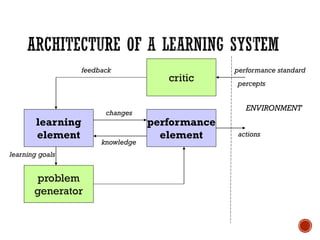
learning
element
critic
problem
generator
performance
element
ENVIRONMENT
feedback
changes
learning goals
actions
percepts
performance standard
knowledge
Design affected by:
▪ performance element used
▪ e.g., utility-based agent, reactive agent, logical agent
▪ functional component to be learned
▪ e.g., classifier, evaluation function, perception-action function,
▪ representation of functional component
▪ e.g., weighted linear function, logical theory, HMM
▪ feedback available
▪ e.g., correct action, reward, relative preferences
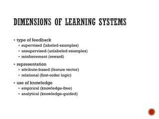
▪ type of feedback
▪ supervised (labeled examples)
▪ unsupervised (unlabeled examples)
▪ reinforcement (reward)
▪ representation
▪ attribute-based (feature vector)
▪ relational (first-order logic)
▪ use of knowledge
▪ empirical (knowledge-free)
▪ analytical (knowledge-guided)
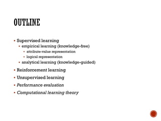
▪ Supervised learning
▪ empirical learning (knowledge-free)
▪ attribute-value representation
▪ logical representation
▪ analytical learning (knowledge-guided)
▪ Reinforcement learning
▪ Unsupervised learning
▪ Performance evaluation
▪ Computational learning theory
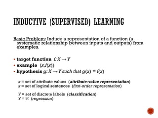
Basic Problem: Induce a representation of a function (a
systematic relationship between inputs and outputs) from
examples.
▪ target function f: X →Y
▪ example (x,f(x))
▪ hypothesis g: X →Y such that g(x) = f(x)
x = set of attribute values (attribute-value representation)
x = set of logical sentences (first-order representation)
Y = set of discrete labels (classification)
Y =  (regression)
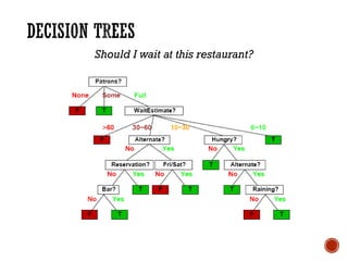
Should I wait at this restaurant?
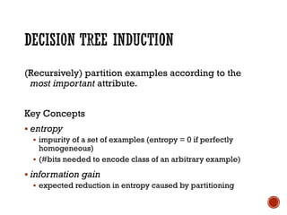
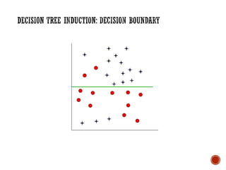
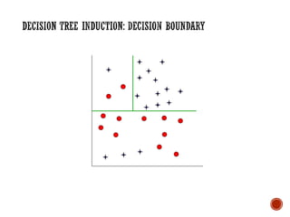
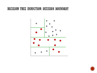
(Recursively) partition examples according to the
most important attribute.
Key Concepts
▪ entropy
▪ impurity of a set of examples (entropy = 0 if perfectly
homogeneous)
▪ (#bits needed to encode class of an arbitrary example)
▪ information gain
▪ expected reduction in entropy caused by partitioning
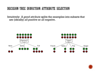
Intuitively: A good attribute splits the examples into subsets that
are (ideally) all positive or all negative.
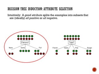
Intuitively: A good attribute splits the examples into subsets that
are (ideally) all positive or all negative.
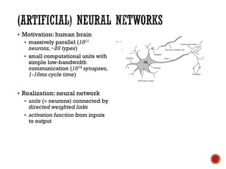
▪ Motivation: human brain
▪ massively parallel (1011
neurons,~20 types)
▪ small computational units with
simple low-bandwidth
communication (1014 synapses,
1-10ms cycle time)
▪ Realization: neural network
▪ units ( neurons) connected by
directed weighted links
▪ activation function from inputs
to output
▪ neural network = parameterized family of nonlinear functions
▪ types
▪ feed-forward (acyclic): single-layer perceptrons, multi-layer networks
▪ recurrent (cyclic): Hopfield networks, Boltzmann machines
[ connectionism,parallel distributed processing]
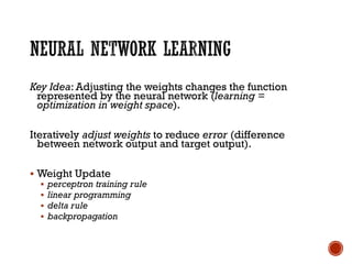
Key Idea: Adjusting the weights changes the function
represented by the neural network (learning =
optimization in weight space).
Iteratively adjust weights to reduce error (difference
between network output and target output).
▪ Weight Update
▪ perceptron training rule
▪ linear programming
▪ delta rule
▪ backpropagation
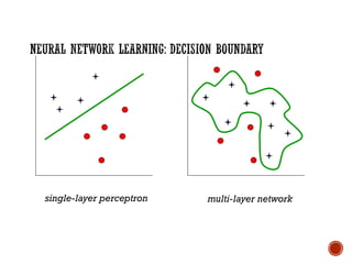
single-layer perceptron multi-layer network
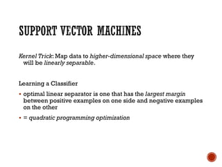
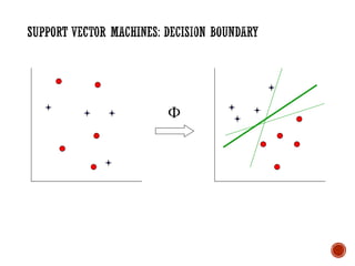
Kernel Trick: Map data to higher-dimensional space where they
will be linearly separable.
Learning a Classifier
▪ optimal linear separator is one that has the largest margin
between positive examples on one side and negative examples
on the other
▪ = quadratic programming optimization
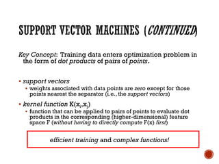
Key Concept: Training data enters optimization problem in
the form of dot products of pairs of points.
▪ support vectors
▪ weights associated with data points are zero except for those
points nearest the separator (i.e., the support vectors)
▪ kernel function K(xi,xj)
▪ function that can be applied to pairs of points to evaluate dot
products in the corresponding (higher-dimensional) feature
space F (without having to directly compute F(x) first)
efficient training and complex functions!
Ф
Network topology reflects
direct causal influence
Basic Task: Compute
probability distribution for
unknown variables given
observed values of other
variables.
[belief networks, causal networks]
A B A B A B A B
C 0.9 0.3 0.5 0.1
C 0.1 0.7 0.5 0.9
conditional probability table
for NeighbourCalls
Key Concepts
▪ nodes (attributes) = random variables
▪ conditional independence
▪ an attribute is conditionally independent of its non-descendants,
given its parents
▪ conditional probability table
▪ conditional probability distribution of an attribute given its parents
▪ Bayes Theorem
▪ P(h|D) = P(D|h)P(h) / P(D)
Find most probable hypothesis given the data.
In theory: Use posterior probabilities to weight
hypotheses. (Bayes optimal classifier)
In practice: Use single, maximum a posteriori (most
probable) hypothesis.
Settings
▪ known structure, fully observable (parameter learning)
▪ unknown structure, fully observable (structural learning)
▪ known structure, hidden variables (EM algorithm)
▪ unknown structure, hidden variables (?)
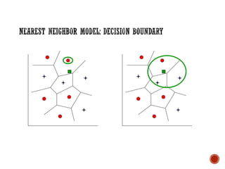
Key Idea: Properties of an input x are likely to be similar to those
of points in the neighborhood of x.
Basic Idea: Find (k) nearest neighbor(s) of x and infer target
attribute value(s) of x based on corresponding attribute
value(s).
Form of non-parametric learning where hypothesis complexity
grows with data (learned model  all examples seen so far)
[instance-based learning, case-based reasoning, analogical reasoning]
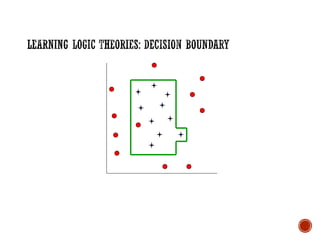
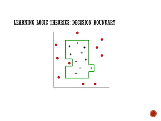
Logical Formulation of Supervised Learning
▪ attribute → unary predicate
▪ instance x → logical sentence
▪ positive/negative classifications → sentences Q(xi),Q(xi)
▪ training set → conjunction of all description and
classification sentences
Learning Task: Find an equivalent logical expression for the
goal predicate Q to classify examples correctly.
Hypothesis  Descriptions ╞═ Classifications
Input
▪ Father(Philip,Charles), Father(Philip,Anne), …
▪ Mother(Mum,Margaret), Mother(Mum,Elizabeth), …
▪ Married(Diana,Charles), Married(Elizabeth,Philip), …
▪ Male(Philip),Female(Anne),…
▪ Grandparent(Mum,Charles),Grandparent(Elizabeth,Beatrice),
Grandparent(Mum,Harry),Grandparent(Spencer,Pete),…
Output
▪ Grandparent(x,y) 
[z Mother(x,z)  Mother(z,y)]  [z Mother(x,z)  Father(z,y)] 
[z Father(x,z)  Mother(z,y)]  [z Father(x,z)  Father(z,y)]
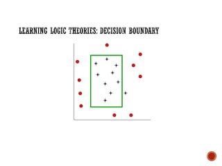
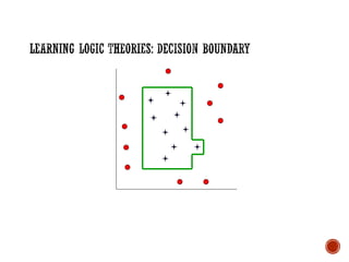
Key Concepts
▪ specialization
▪ triggered by false positives (goal: exclude negative examples)
▪ achieved by adding conditions, dropping disjuncts
▪ generalization
▪ triggered by false negatives (goal: include positive examples)
▪ achieved by dropping conditions, adding disjuncts
Learning
▪ current-best-hypothesis: incrementally improve single
hypothesis (e.g., sequential covering)
▪ least-commitment search: maintain all hypotheses
consistent with examples seen so far (e.g.,version space)
Prior Knowledge in Learning
Recall:
Grandparent(x,y) 
[z Mother(x,z)  Mother)]  [z Mother(x,z)  Father(z,y)] 
[z Father(x,z)  Mother(z,y)]  [z Father(x,z)  Father(z,y)]
▪ Suppose initial theory also included:
▪ Parent(x,y)  [Mother(x,y)  Father(x,y)]
▪ Final Hypothesis:
▪ Grandparent(x,y)  [z Parent(x,z)  Parent(z,y)]
Background knowledge can dramatically reduce the size of
the hypothesis (greatly simplifying the learning problem).
Amazed crowd of cavemen observe Zog roasting a lizard
on the end of a pointed stick (“Look what Zog do!”) and
thereafter abandon roasting with their bare hands.
Basic Idea: Generalize by explaining observed instance.
▪ form of speedup learning
▪ doesn’t learn anything factually new from the observation
▪ instead converts first-principles theories into useful special-
purpose knowledge
▪ utility problem
▪ cost of determining if learned knowledge is applicable may
outweight benefits from its application
Mary travels to Brazil and meets her first Brazilian
(Fernando), who speaks Portuguese. She concludes that
all Brazilians speak Portuguese but not that all Brazilians
are named Fernando.
Basic Idea: Use knowledge of what is relevant to infer new
properties about a new instance.
▪ form of deductive learning
▪ learns a new general rule that explains observations
▪ does not create knowledge outside logical content of prior
knowledge and observations
Medical student observes consulting session between
doctor and patient at the end of which the doctor
prescribes a particular medication. Student concludes
that the medication is effective treatment for a
particular type of infection.
Basic Idea: Use prior knowledge to guide hypothesis
generation.
▪ benefits in inductive logic programming
▪ only hypotheses consistent with prior knowledge and
observations are considered
▪ prior knowledge supports smaller (simpler) hypotheses
k-armed bandit problem:
Agent is in a room with k gambling machines (one-armed bandits).When an arm is
pulled,the machine pays off 1 or 0, according to some unknown probability
distribution. Given a fixed number of pulls, what is the agent’s (optimal) strategy?
Basic Task: Find a policy , mapping states to actions, that maximizes (long-
term) reward.
Model (Markov Decision Process)
▪ set of states S
▪ set of actions A
▪ reward function R : S  A → 
▪ state transition function T : S  A → (S)
▪ T(s,a,s') = probability of reaching s' when a is executed in s
▪ Settings
▪ fully vs. partially observable environment
▪ deterministic vs. stochastic environment
▪ model-based vs. model-free
▪ rewards in goal state only or in any state
value of a state: expected infinite discounted sum of reward the agent
will gain if it starts from that state and executes the optimal policy
Solving MDP when the model is known
▪ value iteration: find optimal value function (derive optimal policy)
▪ policy iteration: find optimal policy directly (derive value function)
Reinforcement learning is concerned with finding an optimal
policy for an MDP when the model (transition, reward) is
unknown.
exploration/exploitation tradeoff
model-free reinforcement learning
▪ learn a controller without learning a model first
▪ e.g., adaptive heuristic critic (TD()), Q-learning
model-based reinforcement learning
▪ learn a model first
▪ e.g., Dyna,prioritized sweeping,RTDP
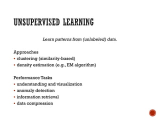
Learn patterns from (unlabeled) data.
Approaches
▪ clustering (similarity-based)
▪ density estimation (e.g., EM algorithm)
Performance Tasks
▪ understanding and visualization
▪ anomaly detection
▪ information retrieval
▪ data compression
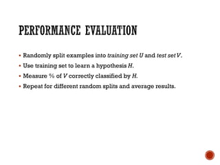
▪ Randomly split examples into training set U and test setV.
▪ Use training set to learn a hypothesis H.
▪ Measure % of V correctly classified by H.
▪ Repeat for different random splits and average results.
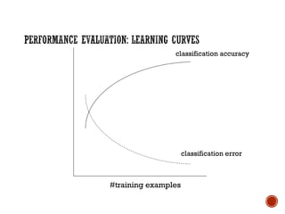
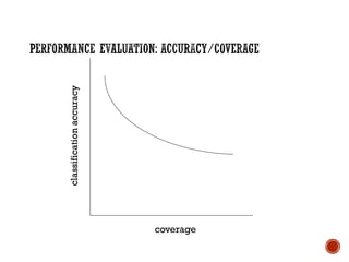
#training examples
classification accuracy
classification error
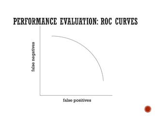
false positives
false
negatives
coverage
classification
accuracy
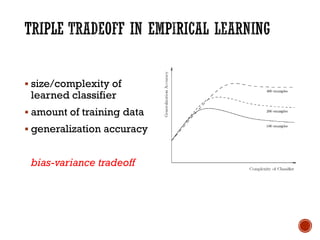
▪ size/complexity of
learned classifier
▪ amount of training data
▪ generalization accuracy
bias-variance tradeoff
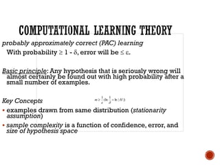
|)
|
ln
1
(ln
1
H
m +



probably approximately correct (PAC) learning
With probability  1 - , error will be  .
Basic principle: Any hypothesis that is seriously wrong will
almost certainly be found out with high probability after a
small number of examples.
Key Concepts
▪ examples drawn from same distribution (stationarity
assumption)
▪ sample complexity is a function of confidence, error, and
size of hypothesis space
▪ Representation
▪ data sequences
▪ spatial/temporal data
▪ probabilistic relational models
▪ …
▪ Approaches
▪ ensemble methods
▪ cost-sensitive learning
▪ active learning
▪ semi-supervised learning
▪ collective classification
▪ …

Buku panduan untuk Machine Learning.pdf

  • 1.
  • 2.
    ▪ AAAI. MachineLearning. http://www.aaai.org/Pathfinder/html/machine.html ▪ Dietterich,T. (2003). Machine Learning.Nature Encyclopedia of Cognitive Science. ▪ Doyle, P. Machine Learning. http://www.cs.dartmouth.edu/~brd/Teaching/AI/Lectures/Summaries/learn ing.html ▪ Dyer, C. (2004). Machine Learning. http://www.cs.wisc.edu/~dyer/cs540/notes/learning.html ▪ Mitchell,T. (1997). Machine Learning. ▪ Nilsson, N. (2004). Introduction to Machine Learning. http://robotics.stanford.edu/people/nilsson/mlbook.html ▪ Russell, S. (1997). Machine Learning. Handbook of Perception and Cognition,Vol. 14, Chap. 4. ▪ Russell, S. (2002). Artificial Intelligence:A Modern Approach, Chap. 18-20. http://aima.cs.berkeley.edu
  • 3.
    ▪ “Learning denoteschanges in a system that ...enable a system to do the same task … more efficiently the next time.” - Herbert Simon ▪ “Learning is constructing or modifying representations of what is being experienced.”- Ryszard Michalski ▪ “Learning is making useful changes in our minds.”- Marvin Minsky “Machine learning refers to a system capable of the autonomous acquisition and integration of knowledge.”
  • 4.
    ▪ No humanexperts ▪ industrial/manufacturing control ▪ mass spectrometer analysis, drug design, astronomic discovery ▪ Black-box human expertise ▪ face/handwriting/speech recognition ▪ driving a car, flying a plane ▪ Rapidly changing phenomena ▪ credit scoring, financial modeling ▪ diagnosis, fraud detection ▪ Need for customization/personalization ▪ personalized news reader ▪ movie/book recommendation
  • 5.
    Machine learning isprimarily concerned with the accuracy and effectiveness of the computer system. psychological models data mining cognitive science decision theory information theory databases machine learning neuroscience statistics evolutionary models control theory
  • 6.
    ▪ rote learning ▪learning by being told (advice-taking) ▪ learning from examples (induction) ▪ learning by analogy ▪ speed-up learning ▪ concept learning ▪ clustering ▪ discovery ▪ …
  • 7.
  • 8.
    Design affected by: ▪performance element used ▪ e.g., utility-based agent, reactive agent, logical agent ▪ functional component to be learned ▪ e.g., classifier, evaluation function, perception-action function, ▪ representation of functional component ▪ e.g., weighted linear function, logical theory, HMM ▪ feedback available ▪ e.g., correct action, reward, relative preferences
  • 9.
    ▪ type offeedback ▪ supervised (labeled examples) ▪ unsupervised (unlabeled examples) ▪ reinforcement (reward) ▪ representation ▪ attribute-based (feature vector) ▪ relational (first-order logic) ▪ use of knowledge ▪ empirical (knowledge-free) ▪ analytical (knowledge-guided)
  • 10.
    ▪ Supervised learning ▪empirical learning (knowledge-free) ▪ attribute-value representation ▪ logical representation ▪ analytical learning (knowledge-guided) ▪ Reinforcement learning ▪ Unsupervised learning ▪ Performance evaluation ▪ Computational learning theory
  • 11.
    Basic Problem: Inducea representation of a function (a systematic relationship between inputs and outputs) from examples. ▪ target function f: X →Y ▪ example (x,f(x)) ▪ hypothesis g: X →Y such that g(x) = f(x) x = set of attribute values (attribute-value representation) x = set of logical sentences (first-order representation) Y = set of discrete labels (classification) Y =  (regression)
  • 12.
    Should I waitat this restaurant?
  • 13.
    (Recursively) partition examplesaccording to the most important attribute. Key Concepts ▪ entropy ▪ impurity of a set of examples (entropy = 0 if perfectly homogeneous) ▪ (#bits needed to encode class of an arbitrary example) ▪ information gain ▪ expected reduction in entropy caused by partitioning
  • 14.
    Intuitively: A goodattribute splits the examples into subsets that are (ideally) all positive or all negative.
  • 15.
    Intuitively: A goodattribute splits the examples into subsets that are (ideally) all positive or all negative.
  • 20.
    ▪ Motivation: humanbrain ▪ massively parallel (1011 neurons,~20 types) ▪ small computational units with simple low-bandwidth communication (1014 synapses, 1-10ms cycle time) ▪ Realization: neural network ▪ units ( neurons) connected by directed weighted links ▪ activation function from inputs to output
  • 21.
    ▪ neural network= parameterized family of nonlinear functions ▪ types ▪ feed-forward (acyclic): single-layer perceptrons, multi-layer networks ▪ recurrent (cyclic): Hopfield networks, Boltzmann machines [ connectionism,parallel distributed processing]
  • 22.
    Key Idea: Adjustingthe weights changes the function represented by the neural network (learning = optimization in weight space). Iteratively adjust weights to reduce error (difference between network output and target output). ▪ Weight Update ▪ perceptron training rule ▪ linear programming ▪ delta rule ▪ backpropagation
  • 23.
  • 24.
    Kernel Trick: Mapdata to higher-dimensional space where they will be linearly separable. Learning a Classifier ▪ optimal linear separator is one that has the largest margin between positive examples on one side and negative examples on the other ▪ = quadratic programming optimization
  • 25.
    Key Concept: Trainingdata enters optimization problem in the form of dot products of pairs of points. ▪ support vectors ▪ weights associated with data points are zero except for those points nearest the separator (i.e., the support vectors) ▪ kernel function K(xi,xj) ▪ function that can be applied to pairs of points to evaluate dot products in the corresponding (higher-dimensional) feature space F (without having to directly compute F(x) first) efficient training and complex functions!
  • 26.
  • 27.
    Network topology reflects directcausal influence Basic Task: Compute probability distribution for unknown variables given observed values of other variables. [belief networks, causal networks] A B A B A B A B C 0.9 0.3 0.5 0.1 C 0.1 0.7 0.5 0.9 conditional probability table for NeighbourCalls
  • 28.
    Key Concepts ▪ nodes(attributes) = random variables ▪ conditional independence ▪ an attribute is conditionally independent of its non-descendants, given its parents ▪ conditional probability table ▪ conditional probability distribution of an attribute given its parents ▪ Bayes Theorem ▪ P(h|D) = P(D|h)P(h) / P(D)
  • 29.
    Find most probablehypothesis given the data. In theory: Use posterior probabilities to weight hypotheses. (Bayes optimal classifier) In practice: Use single, maximum a posteriori (most probable) hypothesis. Settings ▪ known structure, fully observable (parameter learning) ▪ unknown structure, fully observable (structural learning) ▪ known structure, hidden variables (EM algorithm) ▪ unknown structure, hidden variables (?)
  • 30.
    Key Idea: Propertiesof an input x are likely to be similar to those of points in the neighborhood of x. Basic Idea: Find (k) nearest neighbor(s) of x and infer target attribute value(s) of x based on corresponding attribute value(s). Form of non-parametric learning where hypothesis complexity grows with data (learned model  all examples seen so far) [instance-based learning, case-based reasoning, analogical reasoning]
  • 32.
    Logical Formulation ofSupervised Learning ▪ attribute → unary predicate ▪ instance x → logical sentence ▪ positive/negative classifications → sentences Q(xi),Q(xi) ▪ training set → conjunction of all description and classification sentences Learning Task: Find an equivalent logical expression for the goal predicate Q to classify examples correctly. Hypothesis  Descriptions ╞═ Classifications
  • 33.
    Input ▪ Father(Philip,Charles), Father(Philip,Anne),… ▪ Mother(Mum,Margaret), Mother(Mum,Elizabeth), … ▪ Married(Diana,Charles), Married(Elizabeth,Philip), … ▪ Male(Philip),Female(Anne),… ▪ Grandparent(Mum,Charles),Grandparent(Elizabeth,Beatrice), Grandparent(Mum,Harry),Grandparent(Spencer,Pete),… Output ▪ Grandparent(x,y)  [z Mother(x,z)  Mother(z,y)]  [z Mother(x,z)  Father(z,y)]  [z Father(x,z)  Mother(z,y)]  [z Father(x,z)  Father(z,y)]
  • 34.
    Key Concepts ▪ specialization ▪triggered by false positives (goal: exclude negative examples) ▪ achieved by adding conditions, dropping disjuncts ▪ generalization ▪ triggered by false negatives (goal: include positive examples) ▪ achieved by dropping conditions, adding disjuncts Learning ▪ current-best-hypothesis: incrementally improve single hypothesis (e.g., sequential covering) ▪ least-commitment search: maintain all hypotheses consistent with examples seen so far (e.g.,version space)
  • 40.
    Prior Knowledge inLearning Recall: Grandparent(x,y)  [z Mother(x,z)  Mother)]  [z Mother(x,z)  Father(z,y)]  [z Father(x,z)  Mother(z,y)]  [z Father(x,z)  Father(z,y)] ▪ Suppose initial theory also included: ▪ Parent(x,y)  [Mother(x,y)  Father(x,y)] ▪ Final Hypothesis: ▪ Grandparent(x,y)  [z Parent(x,z)  Parent(z,y)] Background knowledge can dramatically reduce the size of the hypothesis (greatly simplifying the learning problem).
  • 41.
    Amazed crowd ofcavemen observe Zog roasting a lizard on the end of a pointed stick (“Look what Zog do!”) and thereafter abandon roasting with their bare hands. Basic Idea: Generalize by explaining observed instance. ▪ form of speedup learning ▪ doesn’t learn anything factually new from the observation ▪ instead converts first-principles theories into useful special- purpose knowledge ▪ utility problem ▪ cost of determining if learned knowledge is applicable may outweight benefits from its application
  • 42.
    Mary travels toBrazil and meets her first Brazilian (Fernando), who speaks Portuguese. She concludes that all Brazilians speak Portuguese but not that all Brazilians are named Fernando. Basic Idea: Use knowledge of what is relevant to infer new properties about a new instance. ▪ form of deductive learning ▪ learns a new general rule that explains observations ▪ does not create knowledge outside logical content of prior knowledge and observations
  • 43.
    Medical student observesconsulting session between doctor and patient at the end of which the doctor prescribes a particular medication. Student concludes that the medication is effective treatment for a particular type of infection. Basic Idea: Use prior knowledge to guide hypothesis generation. ▪ benefits in inductive logic programming ▪ only hypotheses consistent with prior knowledge and observations are considered ▪ prior knowledge supports smaller (simpler) hypotheses
  • 44.
    k-armed bandit problem: Agentis in a room with k gambling machines (one-armed bandits).When an arm is pulled,the machine pays off 1 or 0, according to some unknown probability distribution. Given a fixed number of pulls, what is the agent’s (optimal) strategy? Basic Task: Find a policy , mapping states to actions, that maximizes (long- term) reward. Model (Markov Decision Process) ▪ set of states S ▪ set of actions A ▪ reward function R : S  A →  ▪ state transition function T : S  A → (S) ▪ T(s,a,s') = probability of reaching s' when a is executed in s
  • 45.
    ▪ Settings ▪ fullyvs. partially observable environment ▪ deterministic vs. stochastic environment ▪ model-based vs. model-free ▪ rewards in goal state only or in any state value of a state: expected infinite discounted sum of reward the agent will gain if it starts from that state and executes the optimal policy Solving MDP when the model is known ▪ value iteration: find optimal value function (derive optimal policy) ▪ policy iteration: find optimal policy directly (derive value function)
  • 46.
    Reinforcement learning isconcerned with finding an optimal policy for an MDP when the model (transition, reward) is unknown. exploration/exploitation tradeoff model-free reinforcement learning ▪ learn a controller without learning a model first ▪ e.g., adaptive heuristic critic (TD()), Q-learning model-based reinforcement learning ▪ learn a model first ▪ e.g., Dyna,prioritized sweeping,RTDP
  • 47.
    Learn patterns from(unlabeled) data. Approaches ▪ clustering (similarity-based) ▪ density estimation (e.g., EM algorithm) Performance Tasks ▪ understanding and visualization ▪ anomaly detection ▪ information retrieval ▪ data compression
  • 48.
    ▪ Randomly splitexamples into training set U and test setV. ▪ Use training set to learn a hypothesis H. ▪ Measure % of V correctly classified by H. ▪ Repeat for different random splits and average results.
  • 49.
  • 50.
  • 51.
  • 52.
    ▪ size/complexity of learnedclassifier ▪ amount of training data ▪ generalization accuracy bias-variance tradeoff
  • 53.
    |) | ln 1 (ln 1 H m +    probably approximatelycorrect (PAC) learning With probability  1 - , error will be  . Basic principle: Any hypothesis that is seriously wrong will almost certainly be found out with high probability after a small number of examples. Key Concepts ▪ examples drawn from same distribution (stationarity assumption) ▪ sample complexity is a function of confidence, error, and size of hypothesis space
  • 54.
    ▪ Representation ▪ datasequences ▪ spatial/temporal data ▪ probabilistic relational models ▪ … ▪ Approaches ▪ ensemble methods ▪ cost-sensitive learning ▪ active learning ▪ semi-supervised learning ▪ collective classification ▪ …