The document discusses artificial neural networks and their biological inspiration from networks of neurons in the human brain. It describes how neural networks are built from interconnected simple units that take input and produce output. The perceptron model of a neural network unit is introduced, which learns by modifying connection weights based on errors. Neural networks can represent various functions and problems like handwriting recognition. The backpropagation algorithm is commonly used for training multilayer neural networks by calculating gradients to minimize error.

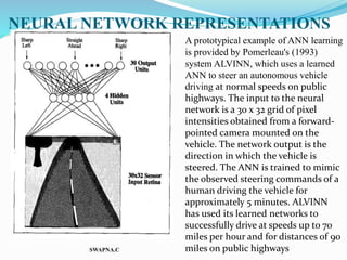
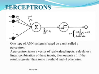
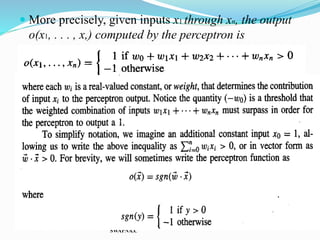
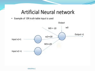
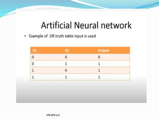
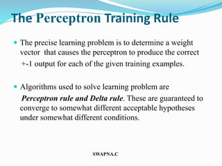
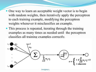
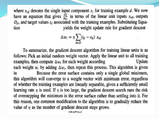
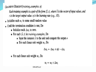
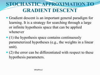
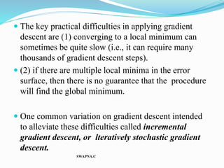
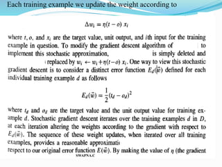
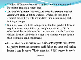
1. By
Swapna.C
Asst.Prof.
IT Dept.
SriDevi Women’s Engineering College
SWAPNA.C

2. INTRODUCTION
 Neural network learning methods provide a robust
approach to approximating real-valued, discrete-
valued, and vector-valued target functions.
 Successful practical problems such as learning to
recognize handwritten characters (LeCun et al.
1989), learning to recognize spoken words (Lang
et al. 1990), and learning to recognize faces
(Cottrell 1990).
SWAPNA.C

3. BIOLOGICAL MOTIVATION
 Artificial neural networks (ANNs) has been inspired in
part by the observation that biological learning systems
are built of very complex webs of interconnected neurons.
 Artificial neural networks are built out of a densely
interconnected set of simple units, where each unit takes a
number of real-valued inputs (possibly the outputs of
other units) and produces a single real-valued output
(which may become the input to many other units).
SWAPNA.C

4.  The human brain, for example, is estimated to contain a
densely interconnected network of approximately 10^11
neurons, each connected, on average, to 10^4 others. Neuron
activity is typically excited or inhibited through connections
to other neurons.
 The fastest neuron switching times are known to be on the
order of 10^-3 seconds--quite slow compared to computer
switching speeds of 10^-10 seconds.
 One motivation for ANN systems is to capture this kind of
highly parallel computation based on distributed
representations.
SWAPNA.C

5.  Historically, two groups of researchers have
worked with artificial neural networks.
 One group has been motivated by the goal of
using ANNs to study and model biological
learning processes.
 A second group has been motivated by the goal of
obtaining highly effective machine learning
algorithms, independent of whether these
algorithms mirror biological processes.
SWAPNA.C

6. SWAPNA.C
Human Brain

7. Neural Network
SWAPNA.C

8. NEURAL NETWORK REPRESENTATIONS
SWAPNA.C
A prototypical example of ANN learning
is provided by Pomerleau's (1993)
system ALVINN, which uses a learned
ANN to steer an autonomous vehicle
driving at normal speeds on public
highways. The input to the neural
network is a 30 x 32 grid of pixel
intensities obtained from a forward-
pointed camera mounted on the
vehicle. The network output is the
direction in which the vehicle is
steered. The ANN is trained to mimic
the observed steering commands of a
human driving the vehicle for
approximately 5 minutes. ALVINN
has used its learned networks to
successfully drive at speeds up to 70
miles per hour and for distances of 90
miles on public highways

9.  ANN approaches, which are based on the
BACKPROPAGATION algorithm .
 The BACKPROPAGATION algorithm assumes the
network is a fixed structure that corresponds to a
directed graph, possibly containing cycles. Learning
corresponds to choosing a weight value for each edge
in the graph.
 Although certain types of cycles are allowed, the vast
majority of practical applications involve acyclic feed-
forward networks, similar to the network structure
used by ALVINN.
SWAPNA.C

10. APPROPRIATE PROBLEMS FOR
NEURAL NETWORK LEARNING
 ANN learning is well-suited to problems in which the training
data corresponds to noisy, complex sensor data, such as inputs
from cameras and microphones.
 The BACKPROPAGATION algorithm is the most commonly
used ANN learning technique. It is appropriate for problems
with the following characteristics:
 Instances are represented by many attribute-value pairs:
 In ALVINN example input attributes may be highly correlated or
independent of one another. Input values can be any real values.
 The target function output may be discrete-valued, real-valued,
or a vector of several real- or discrete-valued attributes:
 In the ALVINN system the output is a vector of 30 attributes, each
corresponding to a recommendation regarding the steering
direction. SWAPNA.C

11.  The training examples may contain errors. ANN
learning methods are quite:
robust to noise in the training data.
 Long training times are acceptable: Network training
algorithms typically require longer training times than,
say, decision tree learning algorithms. Training times can
range from a few seconds to many hours, depending on
factors such as the number of weights in the network, the
number of training examples considered, and the settings
of various learning algorithm parameters.
SWAPNA.C

12. Fast evaluation of the learned target function may be
required:
 Although ANN learning times are relatively long,
evaluating the learned network, in order to apply it to
a subsequent instance, is typically very fast. For
example, ALVINN applies its neural network several
times per second to continually update its steering
command as the vehicle drives forward.
 The ability of humans to understand the learned
target function is not important:
 The weights learned by neural networks are often
difficult for humans to interpret. Learned neural
networks are less easily communicated to humans
than learned rules.
SWAPNA.C

13.  The BACKPROPAGATION Algorithm for training
multilayer networks of such units and consider several
general issues such as the representational capabilities
of ANNs, nature of the hypothesis space search, over
fitting problems, and alternatives to the
BACKPROPAGATION Algorithm.
 A detailed example is also presented applying
BACKPROPAGATION Algorithm recognition, and
directions are provided for the reader to obtain the
data and code to experiment further with this
application.
SWAPNA.C

14. PERCEPTRONS
SWAPNA.C
One type of ANN system is based on a unit called a
perceptron.
A perceptron takes a vector of real-valued inputs, calculates a
linear combination of these inputs, then outputs a 1 if the
result is greater than some threshold and -1 otherwise.

15.  More precisely, given inputs x1 through xn, the output
o(x1, . . . , x,) computed by the perceptron is
SWAPNA.C

16. SWAPNA.C
Representational Power of Perceptions:
We can view the perceptron as representing a hyperplane decision
surface in the n-dimensional space of instances (i.e., points).
The perceptron outputs a 1 for instances lying on one side of the
hyperplane and outputs a -1 for instances lying on the other side.
The equation for this decision
Of course, some sets of positive and negative examples cannot be
separated by any hyperplane. Those that can be separated are
called linearly separable sets of examples.

17. SWAPNA.C
ANN Single Layer Perceptron and Multi Layer Perceptron

18. SWAPNA.C
Perceptron
A single perceptron can be used to represent many boolean functions. For
example, if we assume boolean values of 1 (true) and -1 (false), then one way to
use a two-input perceptron to implement the AND function is to set the weights
wo = -3, and wl = wz = .5. This perceptron can be made to represent the OR
function instead by altering the threshold to wo = -.3. In fact, AND and OR can
be viewed as special cases of m-of-n functions: that is, functions where at least
m of the n inputs to the perceptron must be true. The OR function corresponds
to rn = 1 and the AND function to m = n. Any m-of-n function is easily
represented using a perceptron by setting all input weights to the same value
(e.g., 0.5) and then setting the threshold wo accordingly.

19.  Perceptrons can represent all of the primitive boolean functions
AND, OR, NAND (1 AND), and NOR (1 OR). Unfortunately,
however, some boolean functions cannot be represented by a
single perceptron, such as the XOR function whose value is 1 if
and only if xl # xz.
 The ability of perceptrons to represent AND, OR, NAND, and
NOR is important because every boolean function can be
represented by some network of interconnected units based on
these primitives.
SWAPNA.C

20. SWAPNA.C

21. SWAPNA.C

22. The Perceptron Training Rule
 The precise learning problem is to determine a weight
vector that causes the perceptron to produce the correct
+-1 output for each of the given training examples.
 Algorithms used to solve learning problem are
Perceptron rule and Delta rule. These are guaranteed to
converge to somewhat different acceptable hypotheses
under somewhat different conditions.
SWAPNA.C

23.  One way to learn an acceptable weight vector is to begin
with random weights, then iteratively apply the perceptron
to each training example, modifying the perceptron
weights whenever it misclassifies an example.
 This process is repeated, iterating through the training
examples as many times as needed until the perceptron
classifies all training examples correctly.
SWAPNA.C
Swapna.C

24.  Weights are modified at each step according to the perceptron
training rule, which revises the weight wi associated with input
xi according to the rule
where
Here t is the target output for the current training example, o is
the output generated by the perceptron, and is a positive
constant called the learning rate. The role of the learning rate
is to moderate the degree to which weights are changed at each
step. It is usually set to some small value and is sometimes
made to decay as the no of weights-tuning iterations increases.
SWAPNA.C

25.  Suppose the training example is correctly classified
already by the perceptron. In this case, (t - o) is zero,
making wi zero, so that no weights are updated.
Suppose the perceptron outputs a -1, when the target
output is + 1. To make the perceptron output a + 1
instead of - 1 in this case, the weights must be altered
to increase the value of
SWAPNA.C

26. Gradient Descent and the Delta Rule
 The perceptron rule finds a successful weight vector
when the training examples are linearly separable, it
can fail to converge if the examples are not linearly
separable.
 A second training rule, called the delta rule, is
designed to overcome this difficulty. If the training
examples are not linearly separable, the delta rule
converges toward a best-fit approximation to the target
concept.
 Delta rule also called LMS rule, Adaline rule,
Widrow-Hoff rule.
SWAPNA.C

27. SWAPNA.C

28. VISUALIZING THE HYPOTHESIS SPACE
 The gradient descent algorithm, it is helpful to
visualize the entire hypothesis space of
possible
weight
vectors and
their
associated
E values.
SWAPNA.C

29.  Here the axis wo and w1 represent possible values for
the two weights of a simple linear unit. The wo, w1
plane therefore represents the entire hypothesis
space. The vertical axis indicates the error E relative
to some fixed set of training examples. The error
surface shown in the figure thus summarizes the
desirability of every weight vector in the hypothesis
space.
 Given the way in which we chose to define E, for
linear units this error surface must always be
parabolic with a single global minimum. The specific
parabola will depend, of course, on the particular
set of training examples.
SWAPNA.C

30.  Gradient descent search determines a weight vector
that minimizes E by starting with an arbitrary initial
weight vector, then repeatedly modifying it in small
steps. At each step, the weight vector is altered in the
direction that produces the steepest descent along the
error surface.
 This process continues until the global minimum
error is reached.
SWAPNA.C

31. DERIVATION OF THE GRADIENT DESCENT RULE
SWAPNA.C

32. SWAPNA.C

33.  To construct a practical algorithm for iteratively
updating weights according to Equation we need an
efficient way of calculating the gradient at each step.
 Fortunately, this is not difficult. The vector
of derivatives that form the gradient can be
obtained by differentiating E
SWAPNA.C

34. SWAPNA.C

35. SWAPNA.C

36. STOCHASTIC APPROXIMATION TO
GRADIENT DESCENT
 Gradient descent is an important general paradigm for
learning. It is a strategy for searching through a large
or infinite hypothesis space that can be applied
whenever
 (1) the hypothesis space contains continuously
parameterized hypotheses (e.g., the weights in a linear
unit).
 (2) the error can be differentiated with respect to these
hypothesis parameters.
SWAPNA.C

37.  The key practical difficulties in applying gradient
descent are (1) converging to a local minimum can
sometimes be quite slow (i.e., it can require many
thousands of gradient descent steps).
 (2) if there are multiple local minima in the error
surface, then there is no guarantee that the procedure
will find the global minimum.
 One common variation on gradient descent intended
to alleviate these difficulties called incremental
gradient descent, or lteratively stochastic gradient
descent.
SWAPNA.C

38. Each training example we update the weight according to
SWAPNA.C

39.  The key differences between standard gradient descent and
stochastic gradient descent are:
 In standard gradient descent, the error is summed over all
examples before updating weights, whereas in stochastic
gradient descent weights are updated upon examining each
training example.
 Summing over multiple examples in standard gradient descent
requires more computation per weight update step. On the
other hand, because it uses the true gradient, standard gradient
descent is often used with a larger step size per weight update
than stochastic gradient descent.

SWAPNA.C