Downloaded 1,940 times


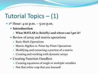

![Review: Array & Matrix Ops (1)
Creating arrays:
No need to allocate memory Easy to create with the
numbers you want Use square braces in between []
array = [1 5 8 7]; Row Vector
array = [1;5;8;7]; Column Vector
Use a space to separate each element
Use a semi-colon (;) to go down to the next row
array = [1 5 8 7]’; Also a column vector
‘ means take the transpose (interchange rows & columns)
After, MATLAB creates an array automatically, with the
values you specified, stored in MATLAB as array](https://image.slidesharecdn.com/advancedmatlabtutorialw2012-120903013858-phpapp02/85/Advanced-MATLAB-Tutorial-for-Engineers-Scientists-12-320.jpg)
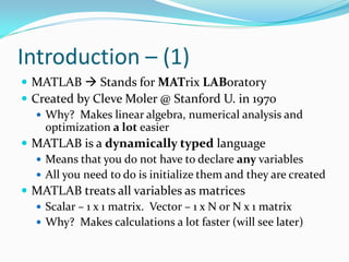
![Review: Array & Matrix Ops (2)
Accessing elements in an array
Use the name of the array, with round brackets ()
Inside the brackets, specify the position of where you
want to access
Remember, MATLAB starts at index 1, not 0 like in C
Examples array = [1 5 8 7];
num = array(2); num = 5
num = array(4); num = 7
Accessing a range of values Use colon (:) operator
Style: val = array(begin:end);
Begin & end are the starting & ending indices to access](https://image.slidesharecdn.com/advancedmatlabtutorialw2012-120903013858-phpapp02/85/Advanced-MATLAB-Tutorial-for-Engineers-Scientists-13-320.jpg)
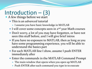
![Review: Array & Matrix Ops (3)
Examples array = [1 5 8 7];
val = array(2:4);
val 3 element array, containing elements 2 to 4 of array
This is equivalent to val = [5 8 7];
val = array(1:2);
val 2 element array, containing elements 1 and 2 of array
This is equivalent to val = [1 5];
We can also access specific multiple elements
val = array([1 4 2 3]);
val A 4 element array: 1st element is from index 1 of array,
2nd element is from index 4 of array, etc.
This is equivalent to val = [1 7 5 8];](https://image.slidesharecdn.com/advancedmatlabtutorialw2012-120903013858-phpapp02/85/Advanced-MATLAB-Tutorial-for-Engineers-Scientists-14-320.jpg)
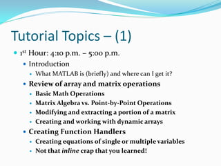
![Review: Array & Matrix Ops (4)
val = array([1 3 2]);
val A 3 element array: 1st element is from index 1 of
array, 2nd element is from index 3 of array, etc.
This is equivalent to val = [1 8 5];
Last thing about arrays
To copy an entire array over, simply set another variable
equal to the array you want to copy
i.e. array2 = array;
This is equivalent to array2 = [1 5 8 7];](https://image.slidesharecdn.com/advancedmatlabtutorialw2012-120903013858-phpapp02/85/Advanced-MATLAB-Tutorial-for-Engineers-Scientists-15-320.jpg)
![Review: Array & Matrix Ops (5)
Let’s move onto matrices
To create a matrix, very much like creating arrays
Use square braces [], then use the numbers you want!
Use spaces to separate between the columns
Use semicolons (;) to go to each row
Example:
M = [1 2 3 4;
M= 5 6 7 8;
9 10 11 12;
13 14 15 16];](https://image.slidesharecdn.com/advancedmatlabtutorialw2012-120903013858-phpapp02/85/Advanced-MATLAB-Tutorial-for-Engineers-Scientists-16-320.jpg)
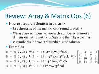
![Review: Array & Matrix Ops (7)
To access a range of values, use the colon operator just
like we did for arrays, but now use them for each
dimension
Examples: M=
B = M(1:3,3:4); Rows 1-3, Cols 3-4
This is equivalent to B = [3 4; 7 8; 11 12];
B = M(3:4,3:4); Rows 3-4, Cols 3-4
This is equivalent to B = [11 12; 15 16];
B = M(1,1:3); Row 1, Cols 1-3
This is equivalent to B = [1 2 3];
B = M(3:4,2); Row 3-4, Col 2
This is equivalent to B = [10;14];](https://image.slidesharecdn.com/advancedmatlabtutorialw2012-120903013858-phpapp02/85/Advanced-MATLAB-Tutorial-for-Engineers-Scientists-18-320.jpg)
![Review: Array & Matrix Ops (8)
Last thing for accessing Using : by itself
Using : for any dimension means to access all values
Examples:
A = M(1:2,:); Rows 1-2, All Cols. M =
Equal to A = [1 2 3 4; 5 6 7 8];
A = M(2,:); Row 2, All Cols.
This is equivalent to A = [5 6 7 8];
A = M(:,3); All Rows, Col 3
This is equivalent to A = [3;7;11;15];
A = M(:,1:3) All Rows, Cols. 1 – 3
Equal to A = [1 2 3; 5 6 7; 9 10 11; 13 14 15];
A = M(:,:); or A = M; Grab the entire matrix](https://image.slidesharecdn.com/advancedmatlabtutorialw2012-120903013858-phpapp02/85/Advanced-MATLAB-Tutorial-for-Engineers-Scientists-19-320.jpg)
![Review: Array & Matrix Ops (11)
Example:
A = [1 2; 3 4];
B = [5 6; 7 8];
E = A + B;
This is equivalent to E = [6 8; 10 12];
F = A – B;
This is equivalent to F = [-4 -4; -4 -4];
G = C + D;
This is equivalent to G = [5 7 9];
H = C – D;
This is equivalent to H = [-3 -3 -3];](https://image.slidesharecdn.com/advancedmatlabtutorialw2012-120903013858-phpapp02/85/Advanced-MATLAB-Tutorial-for-Engineers-Scientists-22-320.jpg)
![Review: Array & Matrix Ops (13)
Examples:
C = A * B;
This is equivalent to C = [19 22; 43 50];
D = A B;
This is equivalent to D = [-3 -4; 4 5];
E = A / B;
This is equivalent to E = [-3 -2; 2 -1];
F = A^2;
This is equivalent to F = [7 10; 15 22];
G = B^3;
This is equivalent to G = [881 1026; 1197 1394];](https://image.slidesharecdn.com/advancedmatlabtutorialw2012-120903013858-phpapp02/85/Advanced-MATLAB-Tutorial-for-Engineers-Scientists-24-320.jpg)
![Review: Array & Matrix Ops (14)
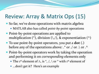
Special case: +,-,* or / every element in a vector or
matrix by a constant number
You use an operation, with the constant number
Examples: A = [1 2; 3 4]; B = [5 6 7 8];
C = 2*A;
This is equivalent to C = [2 4; 6 8];
D = B/3;
This is equivalent to D = [1.6666 2 2.3333 2.6666];
E = A-2;
This is equivalent to E = [-1 0; 1 2];
F = B+4;
This is equivalent to F = [9 10 11 12];](https://image.slidesharecdn.com/advancedmatlabtutorialw2012-120903013858-phpapp02/85/Advanced-MATLAB-Tutorial-for-Engineers-Scientists-25-320.jpg)
![Review: Array & Matrix Ops (16)
Examples:
C = A * B;
This is equivalent to C = [19 22; 43 50];
D = A .* B;
This is equivalent to D = [5 12; 21 32];
E = A B;
This is equivalent to E = [-3 -4; 4 5];
F = A . B;
This is equivalent to F = [5 3; 2.3333 2];
Same as taking every element from B and dividing by its
corresponding element in A](https://image.slidesharecdn.com/advancedmatlabtutorialw2012-120903013858-phpapp02/85/Advanced-MATLAB-Tutorial-for-Engineers-Scientists-27-320.jpg)
![Review: Array & Matrix Ops (17)
Examples:
G = A / B;
This is equivalent to G = [-3 -2; 2 -1];
H = A ./ B;
This is equivalent to H = [0.2 0.3333; 0.4286 0.5];
Same as taking every element from A and dividing by its
corresponding element in B
I = A^2;
This is equivalent to I = [7 10; 15 22];
J = A.^2;
This is equivalent to J = [1 4; 9 16];](https://image.slidesharecdn.com/advancedmatlabtutorialw2012-120903013858-phpapp02/85/Advanced-MATLAB-Tutorial-for-Engineers-Scientists-28-320.jpg)
![Review: Array & Matrix Ops (18)
Now on to modifying elements in arrays and matrices
Do same thing with accessing elements or in groups
Flip the order of what’s on which side of the equals sign
Examples, using the A matrix previously:
A(3,4) = 7; Store 7 in 3rd row, 4th col
A(1:2,3:4) = [5 6; 7 8];
Store this 2 x 2 matrix in Rows 1-2, and Cols 3-4
A(2,:) = [8 19 2 20];
Store this row vector in Row 2
A(:,3) = [5;4;3;2];
Store this column vector in Col 3
A(1:2,:) = 5; Set Row 1-2 and all Cols. to 5](https://image.slidesharecdn.com/advancedmatlabtutorialw2012-120903013858-phpapp02/85/Advanced-MATLAB-Tutorial-for-Engineers-Scientists-29-320.jpg)
![Review: Array & Matrix Ops (19)
Last thing for our review: Dynamic Arrays
Good for not knowing size before hand
We can create arrays that grow in size
We can extend the size and add new elements
You simply set a variable to a set of square braces []
array = [];
After, you just assign numbers to the array
array(1:4) = 5;
array(5:7) = [8 6 8];
array(end+1) = 7; end goes to the end of array,
and +1 puts 7 after the end and extends the size by 1.
Equivalent to array = [5 5 5 5 8 6 8 7];](https://image.slidesharecdn.com/advancedmatlabtutorialw2012-120903013858-phpapp02/85/Advanced-MATLAB-Tutorial-for-Engineers-Scientists-30-320.jpg)
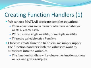
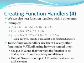
![Creating Function Handlers (5)
Examples:
A = [1 2; 3 4]; B = [2.5 6.7 9];
f = @(x) 5*sin(x) – x.^2 + 3;
g = @(x,y) 25 – x.^2 – y.^2;
a = f(3);
Equivalent to
In MATLAB: a = -5.2944 sin is in radians
b = f(A);
Using same principle, we get:
b = [6.2074 3.5465; -5.2944 -16.7840];
c = g(B,B-2);
Using same principle, this is equivalent to:
c = [18.5 -41.98 -105];](https://image.slidesharecdn.com/advancedmatlabtutorialw2012-120903013858-phpapp02/85/Advanced-MATLAB-Tutorial-for-Engineers-Scientists-35-320.jpg)
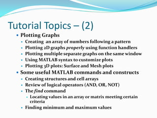
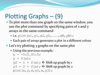
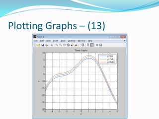
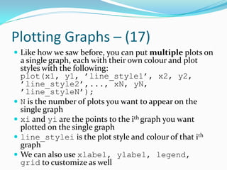
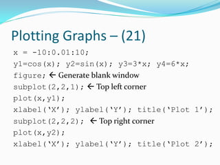
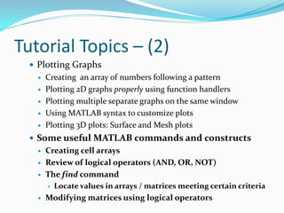
![Plotting Graphs – (2)
Let’s start with 2D plotting:
Assuming that we have two variables, x and y and are
both the same size
To produce the most basic graph in MATLAB that plots
y vs. x, you just do:
plot(x,y);
Let’s start off with a basic example: y = x
We need to generate x and y values first
x = [1 2 3 4 5];
y = [1 2 3 4 5]; or y = x;
plot(x,y);... and we’ll get...](https://image.slidesharecdn.com/advancedmatlabtutorialw2012-120903013858-phpapp02/85/Advanced-MATLAB-Tutorial-for-Engineers-Scientists-38-320.jpg)
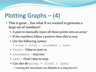
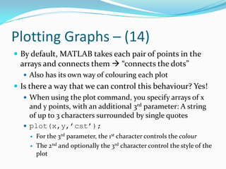
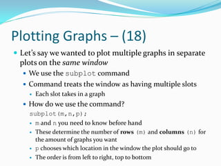
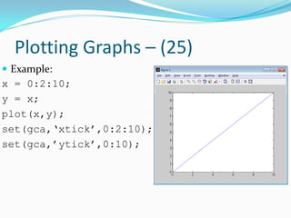
![Plotting Graphs – (5)
Examples:
array = 0 : 2 : 10;
Equivalent to array = [0 2 4 6 8 10];
array = 3 : 3 : 30;
Equivalent to array = [3 6 9 12 15 18 ... 30];
array = 1 : 0.1 : 2.2;
Equivalent to array = [1 1.1 1.2 1.3 ... 2.2];
array = 3 : -1 : -3;
Equivalent to array = [3 2 1 0 -1 -2 -3];
array = 5 : 15;
Equivalent to array = [5 6 7 8 ... 14 15];](https://image.slidesharecdn.com/advancedmatlabtutorialw2012-120903013858-phpapp02/85/Advanced-MATLAB-Tutorial-for-Engineers-Scientists-41-320.jpg)
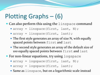
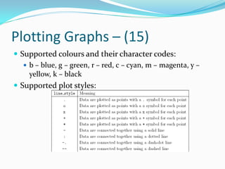
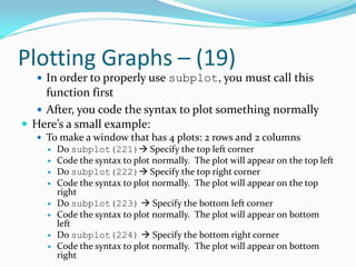
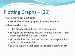
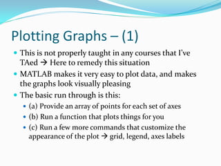
![Plotting Graphs – (27)
How do we generate a grid of x and y values?
Use the meshgrid function
This function will output two matrices, X and Y
X contains what the x co-ordinates are in the grid of
points we want
Y contains what the y co-ordinates are in the grid of
points we want
You need to specify the range of x and y values we want to
plot
[X,Y] = meshgrid(x1:x2,y1:y2);
[X,Y] = meshgrid(x1:inc:x2,y1:inc:y2);](https://image.slidesharecdn.com/advancedmatlabtutorialw2012-120903013858-phpapp02/85/Advanced-MATLAB-Tutorial-for-Engineers-Scientists-63-320.jpg)
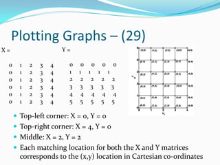
![Plotting Graphs – (28)
x1,x2 determines the beginning and ending x values
respectively
y1,y2 determines the beginning and ending y values
respectively
We can optionally specify inc which specifies the step
size, just like what we’ve seen earlier
Example: [X,Y] = meshgrid(0:4,0:5);
X: Range is from 0 to 4
Y: Range is from 0 to 5](https://image.slidesharecdn.com/advancedmatlabtutorialw2012-120903013858-phpapp02/85/Advanced-MATLAB-Tutorial-for-Engineers-Scientists-64-320.jpg)
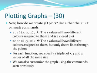
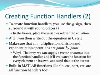
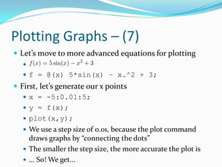
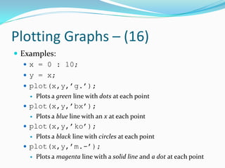
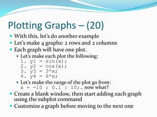
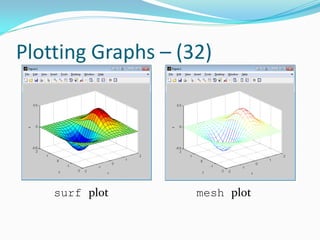
![Plotting Graphs – (31)
Example: Let’s plot the following function
f = @(x,y) x.*exp(-x.^2 – y.^2);
[X,Y] = meshgrid(-2:0.2:2,-2:0.2:2);
Z = f(X,Y); X,Y: Range is from -2 to 2 in steps of 0.2
surf(X,Y,Z); Previous line gets Z points & now plot
xlabel(‘x’); ylabel(‘y’); zlabel(‘z’);
figure; Create a new window
mesh(X,Y,Z); Place mesh graph in new window
xlabel(‘x’); ylabel(‘y’); zlabel(‘z’);](https://image.slidesharecdn.com/advancedmatlabtutorialw2012-120903013858-phpapp02/85/Advanced-MATLAB-Tutorial-for-Engineers-Scientists-67-320.jpg)
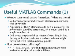
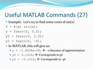
![Useful MATLAB Commands (3)
b = A{2};
Equivalent to b = [1 1 1; 1 1 1; 1 1 1];
C = A(1:2);
Copies elements 1 and 2 from cell array into C
i.e. C{1}=3; C{2}=ones(3,3);
d = A{1};
Equivalent to d = 3;
e = A{3};
Equivalent to e = [0 0 0 0; 0 0 0 0; 0 0 0 0;
0 0 0 0; 0 0 0 0];](https://image.slidesharecdn.com/advancedmatlabtutorialw2012-120903013858-phpapp02/85/Advanced-MATLAB-Tutorial-for-Engineers-Scientists-72-320.jpg)
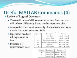
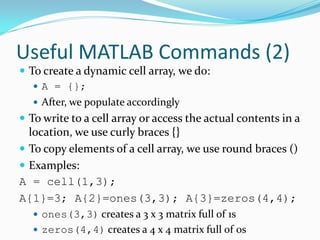
![Useful MATLAB Commands (5)
Let’s take a look at the find command
The find command returns locations of an array or
matrix that satisfy a logical expression
How do we use? index = find(expr);
expr: Logical operator used to find certain values
index: The locations in the array / matrix where
expr is true
Example: A = [1 3 6 2 4];
index1 = find(A >= 4);
Gives: index1 = [3 5]; Locations 3 and 5
Tells us that locations 3 – 5 satisfy this logical expression](https://image.slidesharecdn.com/advancedmatlabtutorialw2012-120903013858-phpapp02/85/Advanced-MATLAB-Tutorial-for-Engineers-Scientists-74-320.jpg)
![Useful MATLAB Commands (6)
index = find(A >= 2 & A <= 4);
Gives: index = [2 4 5];
index = find(A == 3);
Gives: index = 2;
index = find(A ~= 2);
Gives: index = [1 2 3 5];
Using these indices, we can modify arrays / matrices when
certain criteria is met
Examples: A = [1 3 6 2 4]; B = [1 2 3; 4 5 6];
index = find(A >= 2 & A <= 4);
A(ind) = 0; Finds those values between 2 & 4, and set to 0](https://image.slidesharecdn.com/advancedmatlabtutorialw2012-120903013858-phpapp02/85/Advanced-MATLAB-Tutorial-for-Engineers-Scientists-75-320.jpg)
![Useful MATLAB Commands (7)
Now, A = [1 0 6 0 0];
index2 = find(~(B >= 1 & B <= 3));
Find those values that are NOT greater than or equal to
1, and less than or equal to 3.
B(index2) = [9 10 11];
Now, B = [1 2 3; 9 10 11];
One more before we get onto better things
index3 = find(B == 2 | B == 5)
B(index3) = 10;
Now, B = [1 10 3; 4 10 6];](https://image.slidesharecdn.com/advancedmatlabtutorialw2012-120903013858-phpapp02/85/Advanced-MATLAB-Tutorial-for-Engineers-Scientists-76-320.jpg)
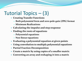
![Useful MATLAB Commands (10)
Example: Let’s say I wanted to create these TFs:
G1(s): Numerator: [2 1], Denominator: [1 2 3 1]
G2(s): Numerator: [5], Denominator: [1 -3 2]
G3(s): Numerator: [10 5 -3], Denominator: [1 5 -4 0 6]
Get it? The numbers that go beside each power of s go
in decreasing order in the square brackets
To specify subtraction, use a negative sign for the #!](https://image.slidesharecdn.com/advancedmatlabtutorialw2012-120903013858-phpapp02/85/Advanced-MATLAB-Tutorial-for-Engineers-Scientists-80-320.jpg)
![Useful MATLAB Commands (11)
Let’s code these transfer function objects
G1 = tf([2 1], [1 2 3 1]);
G2 = tf(5, [1 -3 2]);
G3 = tf([10 5 -3], [1 5 -4 0 6]);
How about ZPK format? Pretty much the same thing
This is the case where we specifically know the what
the poles, zeroes and gain are
Use the zpk command to invoke this style of TF
G = zpk([b0 b1 b2…], [a0 a1 a2…], K);
b0, b1, b2, … are the zero locations
a0, a1, a2, … are the pole locations, and K the gain](https://image.slidesharecdn.com/advancedmatlabtutorialw2012-120903013858-phpapp02/85/Advanced-MATLAB-Tutorial-for-Engineers-Scientists-81-320.jpg)
![Useful MATLAB Commands (12)
Note: We can convert a TF in tf form into zpk form
Example:
G_TF = tf([2 1], [1 2 3 1]);
G_ZPK = zpk(G_TF);
Example: Let’s say I wanted to
create these TFs:
G1(s): zeros: [-2 -3], poles: [-1 -5 -6], gain: 3
G2(s): zeros: [3], poles: [1-i 1+i], gain: 5
G3(s): zeros: [-1], poles: [1 -2], gain: 1
Get it? We can specify imaginary poles / zeroes too!
Factors with addition are negative poles, and vice-versa](https://image.slidesharecdn.com/advancedmatlabtutorialw2012-120903013858-phpapp02/85/Advanced-MATLAB-Tutorial-for-Engineers-Scientists-82-320.jpg)
![Useful MATLAB Commands (13)
Let’s code these transfer function objects
G1 = zpk([-2 -3], [-1 -5 -6], 3);
G2 = zpk(3, [1-i 1+i], 5);
G3 = zpk(-1, [1 -2], 1);
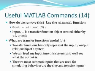
There may be some poles or zeroes that are deemed
insignificant
Their contribution to the overall system will not affect
the output as much
Criteria: If poles and zeroes are very close to each other,
or if any pole or zero is far away from the imaginary axis
To get the best TF, we should remove these](https://image.slidesharecdn.com/advancedmatlabtutorialw2012-120903013858-phpapp02/85/Advanced-MATLAB-Tutorial-for-Engineers-Scientists-83-320.jpg)
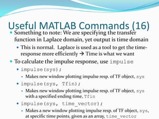
![Useful MATLAB Commands (17)
We can also repeat the same style of invocation by:
[y,t] = impulse(sys);
[y,t] = impulse(sys, Tfin);
[y,t] = impulse(sys, time_vector);
In this way, we don’t generate a plot, but outputs two
arrays: y, the impulse response values, and t, the time
points at each of these values in y
This way is useful if you want to plot more than one
impulse response on the same graph
Use the plot and subplot tools that we’ve seen earlier](https://image.slidesharecdn.com/advancedmatlabtutorialw2012-120903013858-phpapp02/85/Advanced-MATLAB-Tutorial-for-Engineers-Scientists-87-320.jpg)
![Useful MATLAB Commands (18)
To calculate the step response, use the step
command, and we call it exactly in the same style as
impulse
step(sys);
step(sys, Tfin);
step(sys, time_vector);
[y,t] = step(sys);
[y,t] = step(sys, Tfin);
[y,t] = step(sys, time_vector);](https://image.slidesharecdn.com/advancedmatlabtutorialw2012-120903013858-phpapp02/85/Advanced-MATLAB-Tutorial-for-Engineers-Scientists-88-320.jpg)
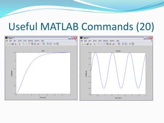
![Useful MATLAB Commands (19)
Example: Let’s try finding impulse and step response with
these two transfer functions
G1 = tf(5, [1 3 2]);
G2 = tf(3, [1 0 25]);
step(G1,7); xlabel(‘Time’); title(‘Step’);
figure; impulse(G2,4);
xlabel(‘Time’); title(‘Impulse’);](https://image.slidesharecdn.com/advancedmatlabtutorialw2012-120903013858-phpapp02/85/Advanced-MATLAB-Tutorial-for-Engineers-Scientists-89-320.jpg)
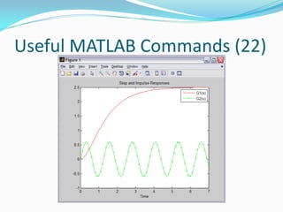
![Useful MATLAB Commands (21)
Let’s try something a bit more advanced
[y1,t1] = step(G1, 0:0.1:7);
[y2,t2] = impulse(G2, 0:0.1:7);
plot(t1,y1,’r-’,t2,y2,’gx-’);
xlabel(‘Time’);
title(‘Step and Impulse Responses’);
legend(‘G1(s)’, ‘G2(s)’);](https://image.slidesharecdn.com/advancedmatlabtutorialw2012-120903013858-phpapp02/85/Advanced-MATLAB-Tutorial-for-Engineers-Scientists-91-320.jpg)
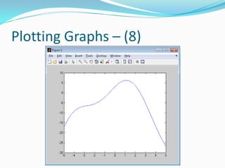
![Useful MATLAB Commands (25)
Examples:
P1 = roots([3 2.5 1 -1 3]);
P2 = roots([5 0 3 -2 0 -1]);
… and we thus get:
P1 = [-0.9195 + 0.8263i; -0.9195 -
0.8263i; 0.5028 + 0.6337i; 0.5028 -
0.6337i];
P2 = [0.7140; -0.0394 + 0.7440i; -0.0394
- 0.7440i; -0.3176 + 0.6354i; -0.3176 -
0.6354i];](https://image.slidesharecdn.com/advancedmatlabtutorialw2012-120903013858-phpapp02/85/Advanced-MATLAB-Tutorial-for-Engineers-Scientists-95-320.jpg)
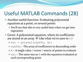
![Useful MATLAB Commands (29)
Example: Let’s evaluate at a variety of
different points
coeffs = [3 5 7];
X = [5 7 9];
val = polyval(coeffs,X);
X2 = [1 2; 3 4];
val2 = polyval(coeffs,X2);
Our outputs are:
val = [107 189 295];
val2 = [15 29; 49 75];](https://image.slidesharecdn.com/advancedmatlabtutorialw2012-120903013858-phpapp02/85/Advanced-MATLAB-Tutorial-for-Engineers-Scientists-99-320.jpg)
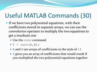
![Useful MATLAB Commands (31)
Example:
When we multiply p, with q, we should get:
When we run this in MATLAB, we’ll see:
P = [1 0 2 4]; Q = [2 0 -1];
A = conv(P,Q);
Now, we will get: A = [2 0 3 8 -2 -4];](https://image.slidesharecdn.com/advancedmatlabtutorialw2012-120903013858-phpapp02/85/Advanced-MATLAB-Tutorial-for-Engineers-Scientists-101-320.jpg)
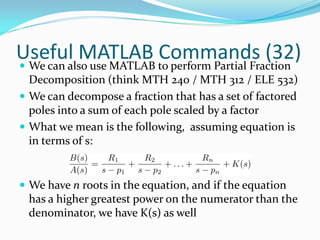
![Useful MATLAB Commands (33)
We call partial fractions by the residue function
[R,P,K] = residue(B,A);
P – the decomposed pole locations (p1,p2,p3…)
R – The scale factors for each of the fractions (R1,R2,R3…)
K – The coefficients of the polynomial equation when
the order of the numerator is greater than the
denominator
If we have repeated roots, then the P and R arrays are
arranged like so:](https://image.slidesharecdn.com/advancedmatlabtutorialw2012-120903013858-phpapp02/85/Advanced-MATLAB-Tutorial-for-Engineers-Scientists-103-320.jpg)
![Useful MATLAB Commands (34)
Which means:
R = [… R(j) R(j+1) … R(j+m-1)…];
P = [… P(j) P(j+1) … P(j+m-1)…];
Example: Let’s find the PFD of
B = [1 -4];
A = [1 6 11 6];
[R,P,K] = residue(B,A);
K = [];
R = [-3.5;6;-2.5];
P = [-3;-2;-1];](https://image.slidesharecdn.com/advancedmatlabtutorialw2012-120903013858-phpapp02/85/Advanced-MATLAB-Tutorial-for-Engineers-Scientists-104-320.jpg)
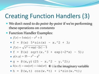
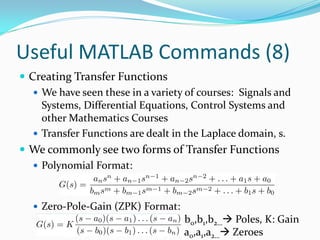
![Useful MATLAB Commands (35)
Couple of things before we take a break:
If we ever wanted to take a small matrix, and repeat it
horizontally and vertically for a finite amount of times,
we can use the repmat command
B = repmat(A,M,N);
M - 1 and N – 1 are the amount of times we want to
repeat the matrix vertically and horizontally respectively
A is the matrix we want to use to repeat
Example:
B =
1 2 1 2 1 2
A = [1 2; 3 4]; 3 4 3 4 3 4
1 2 1 2 1 2
B = repmat(A,2,3); 3 4 3 4 3 4](https://image.slidesharecdn.com/advancedmatlabtutorialw2012-120903013858-phpapp02/85/Advanced-MATLAB-Tutorial-for-Engineers-Scientists-105-320.jpg)
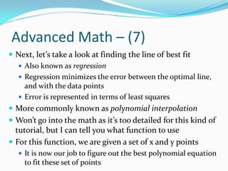
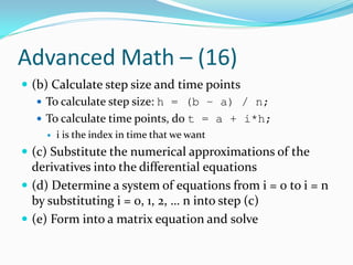
![Advanced Math – (8)
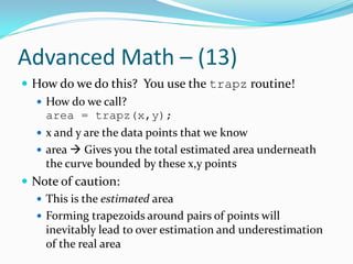
In other words, for our pair of x and y points, we want
to find the co-efficients a0,a1,a2 etc., such that:
How do we do this? Use the polyfit command
A = polyfit(x,y,N);
x and y are our data points Must both be same size!
N is represents the type of polynomial equation we want
N = 1 Linear
N = 2 Parabolic / Quadratic
N = 3 Cubic, etc. etc.
A = [ ];](https://image.slidesharecdn.com/advancedmatlabtutorialw2012-120903013858-phpapp02/85/Advanced-MATLAB-Tutorial-for-Engineers-Scientists-115-320.jpg)
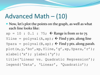
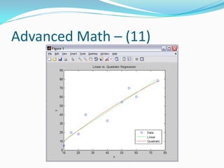
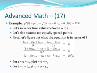
![Advanced Math – (9)
A has the coefficients in decreasing order, just like
what we have seen in tf
Let’s do an example. Let’s say we had the following
data
x = [10 15 20 25 40 50 55 60 75];
y = [5 20 18 40 33 54 70 60 78];
Let’s try fitting a straight line, and a quadratic through
this data by regression
A = polyfit(x,y,1);
B = polyfit(x,y,2);](https://image.slidesharecdn.com/advancedmatlabtutorialw2012-120903013858-phpapp02/85/Advanced-MATLAB-Tutorial-for-Engineers-Scientists-116-320.jpg)
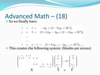
![Advanced Math – (20)
% Create first and last row
X(1,1) = -4;
X(1,2) = 2-h;
X(n,n-1) = 2+h;
X(n,n) = -4;
% Create the rest of the rows
for i = 2 : n-1
X(i,i-1:i+1) = [2+h -4 2-h];
end](https://image.slidesharecdn.com/advancedmatlabtutorialw2012-120903013858-phpapp02/85/Advanced-MATLAB-Tutorial-for-Engineers-Scientists-128-320.jpg)
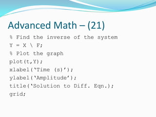
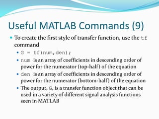
![Advanced MATLAB – (23)
Next advanced function Sorting
Very useful!
If we have an array that we want to sort, use the sort
command
Y = sort(A,’ascend’);
Y = sort(A,’descend’);
[Y,I] = sort(A,’ascend’);
[Y,I] = sort(A,’descend’);
First two sort the array in ascending or descending
order & descending order then place in Y](https://image.slidesharecdn.com/advancedmatlabtutorialw2012-120903013858-phpapp02/85/Advanced-MATLAB-Tutorial-for-Engineers-Scientists-131-320.jpg)
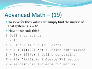
![Advanced MATLAB – (24)
Next two not only give you the sorted array, but it gives
you the indices of where the original values came from
for each corresponding position
Example: A = [1 5 7 2 4];
Y = sort(A,’ascend’);
Y = [1 2 4 5 7];
Y = sort(A,’descend’);
Y = [7 5 4 2 1];
[Y,I] = sort(A,’ascend’);
Y = [1 2 4 5 7]; I = [1 4 5 2 3];
[Y,I] = sort(A,’descend’);
Y = [7 5 4 2 1]; I = [3 2 5 4 1];](https://image.slidesharecdn.com/advancedmatlabtutorialw2012-120903013858-phpapp02/85/Advanced-MATLAB-Tutorial-for-Engineers-Scientists-132-320.jpg)

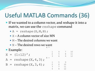
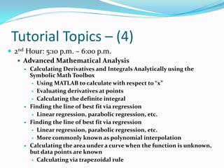
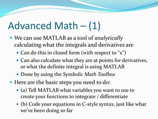
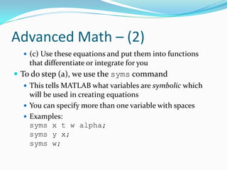
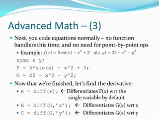
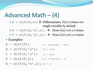
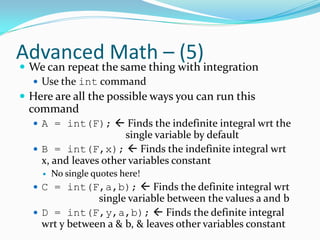
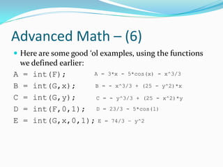
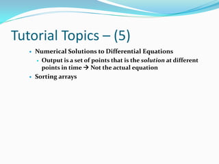
This document outlines a MATLAB tutorial led by Raymond Phan covering various topics such as array and matrix operations, plotting functions, creating transfer functions, and advanced mathematical analysis. It is structured into multiple sections, teaching users how to effectively use MATLAB for numerical methods and mathematical computations. It assumes basic knowledge of MATLAB while also accommodating those with programming experience but no MATLAB exposure.