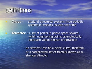
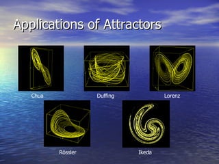
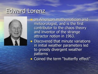
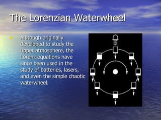
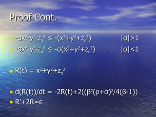
CHAOS Strange Attractors and Lorenz Equations
Definitions Chaos  –  study of dynamical systems (non-periodic    systems in motion) usually over time Attractor  – a set of points in phase space toward    which neighboring points asymptotically    approach within a basin of attraction - an attractor can be a point, curve, manifold   or a complicated set of fractals known as a    strange attractor
Strange Attractor  – an attractor that exhibits  sensitive dependence on initial conditions;  they usually have fractal structure (infinite  detail).  There are several types of strange attractors including: Chua – used in electronic circuitry. Duffing – used in nonlinear oscillators. R össler – used in chemical kinetics. Ikeda – involved in the turbulence of trails of smoke. Lorenz – used in atmospheric convection. Definitions & Applications of Attractors
Applications of Attractors Chua   Duffing   Lorenz R össler   Ikeda
Edward Lorenz an American mathematician and meteorologist, and is the first contributor to the chaos theory and inventor of the strange attractor notion in 1963. Discovered that minute variations in initial weather parameters led to grossly divergent weather patterns Coined the term “butterfly effect”
The Lorenz Attractor is based on three differential equations, three constants, and three initial conditions. The attractor represents the behavior of gas at any given time, and its condition at any given time depends upon its condition at a previous time.  Lorenz Attractor
Although originally developed to study the upper atmosphere, the Lorenz equations have since been used in the study of batteries, lasers, and even the simple chaotic waterwheel. The Lorenzian Waterwheel
Lorenz Equations
The Variables x – refers to the convective flow. y – refers to the horizontal temperature   distribrution. z – refers to the vertical temperature     distribution.
The Constants σ  – sigma refers to the ratio of viscoscity   to thermal conductivity. ρ  – rho refers to the temperature     difference between the top and   bottom of a given slice. β  – beta refers to the ratio of the width to   the height.
Behavior Chaotic behavior can only be found in systems of equations with three or more variables. Within the Lorenz system, there are three things that make the system chaotic. Equations Initial Values Constants If the  ρ  constant is below a certain value, then there will be no chaotic behavior, and the graph will converge.
The Butterfly Effect ^ x solution with respect to time. ^ y solution with respect to time. «  z solution with respect to time.
Proof for Bounded System (x) dx/dt = (- σ x+ σ y)(x) (y) dy/dt = ( ρ x-y-xz) (y) (z n ) dz n /dt = (- β (z n + ρ + σ )+xy) (z n )   ^{z n =z- ρ - σ }   {z=z n + ρ + σ } ½dx 2 /dt =  - σ x 2 + σ xy ½dy 2 /dt =  ρ xy-y2-xy(zn+ ρ + σ ) ½dz n 2 /dt = - β z n 2 - βρ z n - βσ z n +xyz n
Proof Cont. ½d(x 2 +y 2 +z n 2 )/dt = - σ x 2 -y 2 - β z n 2 - β z n ( ρ + σ ) a 2 +b 2  ≥ 2ab 2ab » -z n (√ β -1)(√1/ β -1) β ( ρ + σ ) a 2 +b 2  »  z n 2 ( β -1)+( β 2 ( ρ + σ ) 2 /4( β -1)) ½d(x 2 +y 2 +z n 2 )/dt = - σ x 2 -y 2 -z n 2 + ( β 2 ( ρ + σ ) 2 /4( β - 1))
Proof Cont. - σ x 2 -y 2 -z n 2  ≤ -(x 2 +y 2 +z n 2 )  | σ |>1 - σ x 2 -y 2 -z n 2  ≤ - σ (x 2 +y 2 +z n 2 )  | σ |<1 R(t) = x 2 +y 2 +z n 2 d(R(t))/dt = -2R(t)+2( ( β 2 ( ρ + σ ) 2 /4( β - 1)) R’+2R= ε
Proof Finale R =  ε te -2t +ce -2t R » c  t = 0 R » 0 t »  infinity
The End

Choas Theory3

  • 1.
    CHAOS Strange Attractorsand Lorenz Equations
  • 2.
    Definitions Chaos – study of dynamical systems (non-periodic systems in motion) usually over time Attractor – a set of points in phase space toward which neighboring points asymptotically approach within a basin of attraction - an attractor can be a point, curve, manifold or a complicated set of fractals known as a strange attractor
  • 3.
    Strange Attractor – an attractor that exhibits sensitive dependence on initial conditions; they usually have fractal structure (infinite detail). There are several types of strange attractors including: Chua – used in electronic circuitry. Duffing – used in nonlinear oscillators. R össler – used in chemical kinetics. Ikeda – involved in the turbulence of trails of smoke. Lorenz – used in atmospheric convection. Definitions & Applications of Attractors
  • 4.
    Applications of AttractorsChua Duffing Lorenz R össler Ikeda
  • 5.
    Edward Lorenz anAmerican mathematician and meteorologist, and is the first contributor to the chaos theory and inventor of the strange attractor notion in 1963. Discovered that minute variations in initial weather parameters led to grossly divergent weather patterns Coined the term “butterfly effect”
  • 6.
    The Lorenz Attractoris based on three differential equations, three constants, and three initial conditions. The attractor represents the behavior of gas at any given time, and its condition at any given time depends upon its condition at a previous time. Lorenz Attractor
  • 7.
    Although originally developedto study the upper atmosphere, the Lorenz equations have since been used in the study of batteries, lasers, and even the simple chaotic waterwheel. The Lorenzian Waterwheel
  • 8.
  • 9.
    The Variables x– refers to the convective flow. y – refers to the horizontal temperature distribrution. z – refers to the vertical temperature distribution.
  • 10.
    The Constants σ – sigma refers to the ratio of viscoscity to thermal conductivity. ρ – rho refers to the temperature difference between the top and bottom of a given slice. β – beta refers to the ratio of the width to the height.
  • 11.
    Behavior Chaotic behaviorcan only be found in systems of equations with three or more variables. Within the Lorenz system, there are three things that make the system chaotic. Equations Initial Values Constants If the ρ constant is below a certain value, then there will be no chaotic behavior, and the graph will converge.
  • 12.
    The Butterfly Effect^ x solution with respect to time. ^ y solution with respect to time. « z solution with respect to time.
  • 13.
    Proof for BoundedSystem (x) dx/dt = (- σ x+ σ y)(x) (y) dy/dt = ( ρ x-y-xz) (y) (z n ) dz n /dt = (- β (z n + ρ + σ )+xy) (z n ) ^{z n =z- ρ - σ } {z=z n + ρ + σ } ½dx 2 /dt = - σ x 2 + σ xy ½dy 2 /dt = ρ xy-y2-xy(zn+ ρ + σ ) ½dz n 2 /dt = - β z n 2 - βρ z n - βσ z n +xyz n
  • 14.
    Proof Cont. ½d(x2 +y 2 +z n 2 )/dt = - σ x 2 -y 2 - β z n 2 - β z n ( ρ + σ ) a 2 +b 2 ≥ 2ab 2ab » -z n (√ β -1)(√1/ β -1) β ( ρ + σ ) a 2 +b 2 » z n 2 ( β -1)+( β 2 ( ρ + σ ) 2 /4( β -1)) ½d(x 2 +y 2 +z n 2 )/dt = - σ x 2 -y 2 -z n 2 + ( β 2 ( ρ + σ ) 2 /4( β - 1))
  • 15.
    Proof Cont. -σ x 2 -y 2 -z n 2 ≤ -(x 2 +y 2 +z n 2 ) | σ |>1 - σ x 2 -y 2 -z n 2 ≤ - σ (x 2 +y 2 +z n 2 ) | σ |<1 R(t) = x 2 +y 2 +z n 2 d(R(t))/dt = -2R(t)+2( ( β 2 ( ρ + σ ) 2 /4( β - 1)) R’+2R= ε
  • 16.
    Proof Finale R= ε te -2t +ce -2t R » c t = 0 R » 0 t » infinity
  • 17.